多選題排序應用的演算法

國

立

交

通

大

學

Algorithms for Ranking Responses in Multiple Response Questions

Algorithms for Ranking Responses in Multiple Response Questions

Student

Jia-Ling Ke

Advisor

Hsiuying Wang

A Thesis

Submitted to Institute of Science College of Science National Chiao Tung University in partial Fulfillment of the Requirements

for the Degree of Master

in

Statistics

June 2011

多選題排序應用的演算法

學生：柯佳伶

指導教授

：

王秀瑛 教授

國立交通大學統計學研究所碩士班

摘

要

問卷調查在很多研究中是一項常用的調查工具，其中複選題是問卷中常見到

的題型。近年來，很多研究提出了一些模型和方法針對複選題的資料做分析，但

複選題選項排序的問題是目前主要有興趣的議題。Wang (2008) 提出了一些方法

用來檢定任兩個選項被選到的機率是否相等，然而，當選項的個數太多時，根據

這些方法來做排序將會使得排序過程變得複雜費時。因此，在本篇文章裡，我們

提出了一個演算法進而寫成一個程式，使得不管選項個數的多寡，都能迅速排序

出結果。此外，為了減少排序上不一致性問題的情況發生，我們提出採用 False

Discovery Rate 的檢定準則來做排序。根據我們模擬的結果，證明這樣的方法可

以減少不一致性現象的出現。

ii ii

Algorithms for Ranking Responses in Multiple Response Questions

student：Jia-Ling Ke

Advisors：Dr. Hsiuying Wang

Institute of Statistics

National Chiao Tung University

ABSTRACT

In many studies, the questionnaire is a common tool for surveying. A multiple

response question is a commonly used question designed in a questionnaire. Recently,

many studies proposed models and approaches for analyzing data of a multiple

response question. Ranking responses problem may be the primary issue in the

analysis of a multiple response question. Wang (2008) proposed methodologies for

testing the equality of selected probabilities for two responses. Since it is possible that

the number of responses is large, it leads to a complicated situation to rank the

responses based on these approaches. In this study, we develop algorithms for ranking

responses for any response number. In addition, to diminish the ranking inconsistent

situation, we propose adopting the false discovery rate testing criterion for ranking. A

simulation study shows it can reduce the frequency of ranking inconsistent

phenomenon.

Keywords: single response question; multiple response question; Wald test;

iii iii

誌

謝

短短的兩年碩士生涯轉眼即過，時間雖然短暫，但卻收穫不少，最開心的莫

過於能夠順利地完成論文。本篇論文得以順利完成，首先要感謝我的指導教授-王秀瑛教授，感謝您在論文研究上總是不厭其煩地指導與耐心校正，平時也不時

地關心學生，無論是在課業、生活或是未來就業上。其次，感謝口試委員洪慧念

教授、吳謂勝教授及鄭又仁教授辛苦審查，並給予指導與建議，引領我更周延的

思考，使論文更嚴謹完善。

感謝一起畢業的同學們，很開心可以認識大家，雖然相處的時間不算長，但

卻一起創造許多美好難忘的回憶。寫論文的這段時間，幸好有大家互相的鼓勵打

氣，才能度過撰寫論文的煎熬。

最後，感謝我最親愛的家人，謝謝你們總是在背後支持我鼓勵我，並給予我

無限的關懷，讓我能無後顧之憂順利完成碩士學位。

柯佳伶 謹誌于

國立交通大學統計研究所

中華民國一百年六月

Contents

1 Introduction 1

2 Preliminaries 4

2.1 Wald Test . . . 4 2.2 Generalized Score Test . . . 5 2.3 Likelihood Ratio Test . . . 5

3 Ranking Rule and Algorithm 6

3.1 Rule . . . 6

4 Ranking Inconsistency 8

4.1 False Discovery Rate . . . 8 4.2 Simulation Result . . . 9

5 A Real Data Example 11

6 Conclusion 13

A Flowchart of The Ranking Rule 14

B R Code User Manual 15

C R-codes 18

List of Tables

1 Random variables related to m hypothesis tests. . . 9

2 The number of the responses be chosen. . . 10

3 The statistics and p-values. . . 11

List of Figures

1

Introduction

Questionnaires are important tools for surveying in many studies. They are especially important in marketing or management studies. There are usually two kinds of ques-tions: single response questions and multiple response questions. The analyses of single response questions have been investigated in the literature. However, the analyses of mul-tiple response questions have not been discussed in depth like single response questions until recently. Umesh (1995) first discussed the problem of analyzing multiple response questions. Subsequently, Loughin and Scherer (1998), Decady and Thomas (1999) and Bilder, Loughin and Nettleton (2000) proposed several methods for testing marginal in-dependence between a single response question and a multiple response question. Agresti and Liu (1999,2001) discussed the modeling of multiple response questions. These studies mainly focused on the analysis of the dependence between a single response question and a multiple response question. However, in practice, most researchers are also interested in ranking responses to a question according to the probabilities of responses being chosen. In fact, the ranking responses problem may be the primary issue in the analysis of a survey.

Wang (2008) propose several testing methods to test the equality of the probabilities of responses being selected in a multiple response question, including the wald test, score test and the likelihood ratio test. A ranking guide is giving in Wang (2008) based on the testing results to rank the responses. However, in real applications, it is common that there are more than 10 responses in a multiple response question. When the number of responses is large, it is not straightforward to apply the guide to rank the responses. In this study, we mainly provide a rule and programming to rank the responses for any number of responses.

In addition, except adopting the wald test for ranking, we propose using false discovery rate criterion to rank responses. As pointed out in Wang (2008), a reasonable approach should have the ranking consistent property. However, the wald test, score test and

likelihood ratio test do not have the ranking consistent property. To reduce the frequency of ranking inconsistency, the false discovery rate criterion is used to to be an alternative approach. From a simultaneous study, we find that the false discovery rate method can diminish the frequency of ranking inconsistent situation occurrence. Therefore, it is a potential competitor for ranking responses.

We first illustrate the model using the following example. For instance, a company is designing a marketing survey to help develop a body lotion product. The researchers will design a multiple response question and list several factors, including price, effect, brand, ingredients and smell that could attract consumers to purchase it. Suppose that a group of individuals are surveyed on purchasing a body lotion. They are asked to fill out questionnaires which list all the questions that we wish to address to each respondent. The following is a multiple response question in the questionnaire:

Question 1. Which factors are important to you when considering the purchase of a body lotion? (1) price (2) effect (3) brand (4) ingredients (5) smell.

Assume that according to the number of each response being chosen, most respondents are more concerned about the price and the effect than the other factors of the product. Then we may rank the response “price” first and “effect” second according to the number of responses selected. However, only basing on the response selected numbers to rank responses is not statistically significant and we cannot confidently claim that the factor “price” is more important than the factor “effect”. In this study, we are interested in developing algorithms to rank all responses based on statistical testing approaches.

First, we focus on ranking two specific responses that we are interested in. For the general case, assuming that a multiple response question has k responses, v1, · · · , vk, and

we interview n respondents. Each respondent is asked to choose at least one and at most s answers for this question, where 0 < s ≤ k. If s = 1, it is a single response question. There are a total of c = Ck

1 + · · · + Csk possible kinds of answers that respondents will

choose. Let ni1···ik denote the number of respondents selecting the responses vh and not

selecting vh0 if i_h = 1 and i_h0 = 0, and p_i

1···ik denotes the corresponding probability.

and the fifth responses and not slecting the other responses. Thus, the pmf function of n∗ = {ni1···ik, ij = 0 or 1, and k P j=1 ij ≤ s} is fs(ni1···ik) = I( k X j=1 ij ≤ s) n! Q ij=0 or 1 ni1···ik! Y ij=0 or 1 pn_ii1···ik 1···ik , (1)

where I(·) denotes the indicator function. Let mj denote the sum of the number ni1···ik

such that the jth response is selected, and πj denote the corresponding probability, that is

mj = P ij=1

ni1···ik and πj =

P

ij=1

pi1···ik. Note πj is called a marginal probability of response

j. Also let mjl denote the sum of the number ni1,···ik such that the jth and lth responses

are selected, and πjl denote the corresponding probability. Then mjl = P ij=il=1

ni1···ik and

πjl= P ij=il=1

pi1···ik.

For ranking the importance of two specified responses, say response 1 and response 2 in Question 1 from the survey data, we will consider the two-sided test:

H0 : π1 = π2 vs H1 : π1 6= π2, (2)

which is equivalent to

H₀∗ : π1 − π12 = π2 − π12 vs H1∗ : π1− π126= π2− π12. (3)

If (2) is rejected, then we can rank the response with larger mj first.

The methods for testing (2) are given in Wang (2008). In this study, we propose an algorithm based on these testing approaches to rank the responses. This algorithm can successfully rank responses to several clusters.

Although the algorithm based on testing approaches proposed in Wang (2008) can suc-cessfully rank the responses. The testing approaches suffer the drawback of the ranking inconsistent property (Wang 2008). Since these testing approaches have ranking incon-sistent property, we intend to diminish the frequency of ranking inconincon-sistent situations. Therefore, we propose using a false discovery rate testing method to replacing the testing method. From a simulation study, the false discovery rate criterion is shown to successfully reduce the frequency of ranking inconsistent situations.

This thesis is organized as follows. In Section 2, the three testing methods for testing (2) are reviewed. The proposed algorithm based on testing approaches in Wang (2008) is given in Section 3. We review the ranking inconsistent property and propose a false discovery rate method in Section 4. Finally, a real data example is given to illustrate the proposed methods.

2

Preliminaries

Before proposing a rule for ranking all responses in a multiple response question, we have to know how to solve the problem of ranking the two specific responses. In this section, we will review the literature which was presented by Hsiuying Wang (2008). In the literature, the professor first proposed three methods for testing whether there are significant differences in two specific responses, i.e. it was used for testing (2).

2.1

Wald Test

A Wald test is a test based on a statistic of the form Zn =

Wn− (π1− π2)

Sn

,

where Wn is an estimator of π1 − π2, and Sn is a standard error for Wn. An unbiased

estimator of pi1,··· ,ik is ni1,··· ,ik/n, which is also a maximum likelihood estimator (MLE).

Let ˆπ1 = m1/n, ˆπ2 = m2/n and ˆπ12 = m12/n. We can use ˆπ1 = m1/n and ˆπ2 = m2/n as

estimators of π1 and π2 respectively,and we have

V ar ( ˆπ1− ˆπ2) =        π1(1 − π1)/n + π2(1 − π2)/n + 2π1π2/n if s = 1 (π1− π12)(1 − π1+ 2π2− π12)/n+ (π2− π12)(1 − π2+ π12)/n otherwise. (4)

Under the null hypothesis H0 in (2) and based on the central limit theorem, the

statistics

ˆ π1− ˆπ2

pV ar( ˆπ1− ˆπ2)

(5) converges in distribution to a standard normal random variable when n is large. Since π1, π2 and π12 are unknown, we can use ˆπ1, ˆπ2 and ˆπ12to substitute π1, π2 and π12 in (4).

Thus, for testing (2), H0 is rejected if the absolute value of (5) is greater than zα₂, where

zα

2 is the upper α/2 cutoff point of the standard normal distribution.

2.2

Generalized Score Test

In Section 2.1, π1, π2 and π12 in V ar( ˆπ1 − ˆπ2) are replaced by ˆπ1, ˆπ2 and ˆπ12 in the

test statistic. In this section, we consider the variance under the null hypothesis in (2), that is, π1 = π2. Thus, we have

V arπ1=π2( ˆπ1− ˆπ2) =    2π1/n if s = 1 2(π1− π12)/n. otherwise. (6) By the central limit theorem, under H0, the statistic

( ˆπ1− ˆπ2)/

p

V arπ1=π2( ˆπ1− ˆπ2)

coverges to a standard normal distribution when n is large. We can use ( ˆπ1+ ˆπ2) /2 and

ˆ

π12as substitutes for π1 and π12in the variance. Hence, for testing (2), the null hypothesis

is rejected if      √ n∗| ˆπ1− ˆπ2| √ ˆ π1+ ˆπ2 > zα/2 if s = 1, √ n∗| ˆπ1− ˆπ2| √ ( ˆπ1+ ˆπ2−2ˆπ12) > zα/2 if 1 < s ≤ k. (7)

This approach is similar to the score test of testing a marginal probability equal to a specified value. Hence we call this approach a generalized score test.

2.3

Likelihood Ratio Test

The third approach is the likelihood ratio test (LRT). For testing H0 : π1 = π2, let

Λ12 =

L(ˆpˆi1···ik)

L(ˆpi1···ik)

, (8)

where L is the likelihood function, and ˆpˆi1···ik and ˆpi1···ik denote the MLE of pi1···ik under

the restricted parameter space π1 = π2and the whole parameter space, respectively. Thus,

we have

ˆ

When s = 1, ˆ ˆ pi1···ik =    (n100···0+ n010···0)/(2n) if i1 = 1 (n100···0+ n010···0)/(2n) if i2 = 1 ni1···ik/n otherwise, (9) which is easily to be interpreted because under π1 = π2, ˆpˆ10···0 and ˆpˆ20···0 should be equal

to (ˆp10···0+ ˆp010···0)/2.

When 1 < s ≤ k, by solving the equations of derivatives of the likelihood ratio functions with respect to pi1···ik being zero, we have

ˆ ˆ pi1···ik =    S · ni1···ik/(2n( P i1=1,i2=0ni1···ik)) if i1 = 1, i2 = 0 S · ni1···ik/(2n( P i1=0,i2=1ni1···ik)) if i1 = 0, i2 = 1 ni1···ik/n otherwise, (10) where S = X i1=1,i2=0 ni1···ik+ X i1=0,i2=1 ni1···ik.

According to the asymptotic theory of the likelihood ratio test, −2logΛ12has a limiting

distribution with one degree of freedom. For testing (2), H0 is rejected if

−2logΛ12> χ21,α,

where χ2

1,αis a upper α cutoff point of chi-square distribution with one degree of freedom.

3

Ranking Rule and Algorithm

In this section, we focus on how to use these three testing methods to rank all responses. Since the method of Likelihood ratio test is more complicated to calculate than the other two methods, we only use the method of Wald test or Score test to rank all responses, But in this paper we focus on using Wald test. First we propose a rule for ranking all responses as follows.

3.1

Rule

Assume that we have k responses, and first we have to compute each mj, j = 1, j =

the response corresponding to m(j). It is natural to rank the importance of responses

in order of m(j). That is, the most influential response is v(k), and the second influential

response is v(k−1). However, ranking responses based on the order of mj is not statistically

significant. The proposed testing methods in Section 2 can be used to rank the responses. If the hypothesis π(k) = π(k−1) is rejected, where π(r) denotes the marginal probability

corresponding to v(r), then we may claim that v(k) is the most influential response. If it

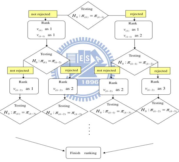
is not rejected, then we compare v(k) with v(j), j ≤ k − 2 sequentially. A ranking rule is

proposed in this study. The flowchart of the rule is given in Figure 1 of Appendix A. We use Question 1 as an example to illustrate the rule. For example, m1 = 47, m2 =

35, m3 = 17, m4 = 19, m5 = 30, and then m(1) = 17, m(2) = 19, m(3) = 30, m(4) =

35, m(5) = 47. It is nature to rank the importance of responses in order of m(j). We may

claim that the factor of price is more importan than the factor of effect for consumers to purchase. However, ranking response only based on the magnitudes of mj, is not

statistically significant. Hence, we follow the proposed rule and use one of the three methods to rank all responses. First, we rank response v(5) and response v(4), i.e. rank

the response (1) and response (2). If H0 : π(5) = π(4) is not rejected, but H0 : π(5) = π(3)

is rejected, it means that the response (1) and response (2) are equally important, but they are more important than response (5). And then we will compare π(3) with π(2). If

H0 : π(3) = π(2) is rejected, and then testing H0 : π(2) = π(1). If it is not rejected, the

result of ranking is to rank response (1) and (2) first, response (5) second, and response (2) and (3) third. We denote the ranking notations for the above result as (1) 1 (2) 1 (3) 3 (4) 3 (5) 2 . Hence, we can know that response (1)-price and response (2)-effect are top priorities when consumers purchase a body lotion, response (5)-smell is the second important factor, and response (3)-brand and response (4)-ingredients are relatively unimportant for consumers.

Following the rule we can rank the importance of all response in a multiple response question, but it is more complicated and not easy to do when there are many responses in a multiple response question. Hence, we will provide an algorithm for ranking. The algorithm is a R code which is included in the Appendix C. The manual for using the

code is also provided in the Appendix B.

4

Ranking Inconsistency

According to the rule of ranking responses, a reasonable test should have the following property: if H0 : π(j) = π(i), i ≤ j is rejected by test, then H0 : π(j) = π(g), g < i should

also be rejected by the test with the same level because |m(j)− m(i)| < |m(j) − m(g)|.

We call this property ranking consistency. If a test has ranking consistent property, we call it a ranking consistent test. The algorithm we proposed in Section 3 is under the assumption of ranking consistency. However, in the multiple response question case, this ranking consistent property is not valid for all data, but the frequency of the ranking inconsistent phenomenon occurrence is low according to the simulation results.

4.1

False Discovery Rate

To reduce the frequency of ranking inconsistent phenomenon occurrence we propose us-ing false discovery rate approach. Assume that there are k responses and we are interested in testing

H0k−1: π(k) = π(k−1) vs H1k−1: π(k) 6= π(k−1)

H0k−2: π(k) = π(k−2) vs H1k−2: π(k) 6= π(k−2)

· · ·

H01: π(k) = π(1) vs H11 : π(k) 6= π(1) (11)

Since it is a multiple hypothesis testing, we try to use false discovery rate (FDR) method to improve the problem of ranking inconsistency.

False discovery rate (FDR) control is a statistical method used in multiple hypothesis testing to correct for multiple comparisons. In a list of rejected hypotheses, FDR controls the expected proportion of incorrectly rejected null hypotheses (Type I errors). The false discovery rate is given by E[_{V +S}V ] and one wants to keep this value below a threshold α.

Table 1: Random variables related to m hypothesis tests.

Null hypothesis is true Alternative hypothesis is true Total

Declared significant V S R

Declared non-significant U T m − R

Total m0 m − m0 m

• m is the total number hypotheses tested. • m0 is the number of true null hypotheses.

• m − m0 is the number of true alternative hypotheses.

• V is the number of false positives (Type I error). • S is the number of true positives.

• T is the number of false negatives (Type II error). • U is the number of true negatives.

• In m hypothesis tests of which m0 are true null hypotheses, R is an observable

random variable, and S, T , U , and V are unobservable random variables.

The FDR procedure proposed by Benjamini and Hochberg (1995) ensures that its expected value E[_{V +S}V ] is less than a given α. This procedure is valid when the m tests are independent. Let H1, · · · , Hm be the null hypotheses and p1, · · · , pm be their

corre-sponding p-values. Let p(1), · · · , p(m) denote the order statistics. For a given α, find the

largest c such that

p(c) ≤

c mα Then reject all H(i) for i = 1, · · · , c.

4.2

Simulation Result

This simulation study is conducted to prove that the inconsistent situation is reduced by applying FDR criterion for multiple hypothesis testing. The simulation procedure is to generate a set of p∗ = {pi1···ik, ij = 0 or 1} and then generate a sample from (1)

based on the generated p∗ . Then we can use the sample to check the ranking consistent property of the usual and FDR criterion. Here we repeat the simulation process 10000

times. According to the result, we can find the ratio of ranking inconsistent phenomenon occurrence to the total sample number 10000 is 0.0012 by using fixed α, while the ratio is 0.0007 by using FDR. Hence we can claim that the FDR criterion can reduce the fre-quency of ranking inconsistent phenomenon occurrence. Example 5.1 gives an example which is ranking inconsistent using the usual criterion and is ranking consistent using FDR criterion.

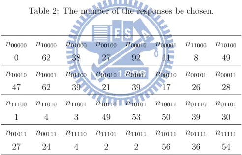
Example 5.1: Assume that a multiple response question has five answers. The data are presented in Table 2. The p-value for testing (2) by Wald test are given in Table 3 :

Table 2: The number of the responses be chosen.

n00000 n10000 n01000 n00100 n00010 n00001 n11000 n10100 0 62 38 27 92 11 8 49 n10010 n10001 n01100 n01010 n01001 n00110 n00101 n00011 47 62 39 21 39 17 26 28 n11100 n11010 n11001 n10110 n10101 n10011 n01110 n01101 1 4 3 49 53 50 39 30 n01011 n00111 n11110 n11101 n11011 n10111 n01111 n11111 27 24 4 2 2 56 36 54

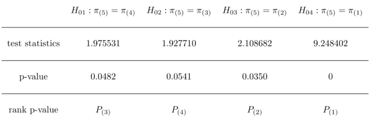
Table 3: The statistics and p-values.

H01: π(5)= π(4) H02: π(5)= π(3) H03: π(5)= π(2) H04: π(5)= π(1)

test statistics 1.975531 1.927710 2.108682 9.248402

p-value 0.0482 0.0541 0.0350 0

rank p-value P(3) P(4) P(2) P(1)

First we consider the usual case that the Type I error is fixed to be 0.05 (α=0.05) For testing H01, since the p-value 0.0482 < α, H01 is rejected. We expect that H02should

also be rejected. However, for testing H02, the p-value 0.0541 > α, which does not reject

H02. Hence, the test is ranking inconsistency.

Then we apply FDR method in the example. Since P(1) < 1₄ × 0.05 = 0.0125, but

P(2) > 2₄ × 0.05 = 0.025, so according to FDR method, only H04 was rejected. Hence, we

can claim that the test is ranking consistency.

From example 5.1, we can know that FDR is a better method for solving the problem of ranking inconsistency.

However, the algorithm based on false discovery rate is more complicated than the usual testing criterior and is still under investigation.

5

A Real Data Example

In this section, we use a real data example to illustrate the proposal rule. This example is a survey of 49609 first-year college students in Taiwan about their preferences in their college study. The data set can be accessed at http://srda.sinica.edu.tw . We list one of the multiple response questions in the questionnaire as follows:

Question: What kind of experience do you expect to receive during the period of college study? (Please select at least one response)

1. Read over the Chinese and foreign classic literature. 2. Travel around Taiwan.

3. Present academic papers in conferences. 4. Lead large-scale activities.

5. Be on a school team.

6. Be a cadre of student associations. 7. Participate internship programs. 8. Fall in love.

9. Have sexual experience. 10. Travel around the world. 11. Make many friends. 12. Others.

We are interested in ranking all responses of this multiple response question accord-ing to students’ preference. The population is all first-year college students in Taiwan. The projectors sampled 49609 first-year college students form the population to fill out the questionnaire. Since there are many missing data in the whole data set, we have to delete the missing data. Then real sample size is 3388. Since we have all data, we can obtain the ranks of the twelve responses by the order of mj. Note that from the

whole data set, the numbers of respondents selecting the twelve responses we denoted by m1 = 623, m2 = 1889, m3 = 338, m4 = 913, m5 = 637, m6 = 1134, m7 = 1596, m8 =

1660, m9 = 531, m10 = 1556, m11= 2699, m12 = 118. Since it’s risky to rank all responses

basing only on the order of mj, we have to use the rule and program for ranking all

responses.

To implement our program, we need to construct survey data and set α=0.05. Input these parameters into the function in our program, we can obtain the result of ranking all responses is (1) 7 (2) 2 (3) 9 (4) 6 (5) 7 (6) 5 (7) 3 (8) 3 (9) 8 (10) 4 (11) 1 (12) 10 . From the result we can claim that the first-year college students prefer to ”make many friends”, ” travel around Taiwan”, ”participate internship programs”, and ”fall in

love”, where ”participate internship programs” and ”fall in love” are equally important and ranked third for the students.

From the this real data example, we can verify that the program we proposed is feasible and convenient in practice when we want to rank all responses in a multiple response question.

6

Conclusion

The questionnaire is an important tool for surveying. Ranking the responses in a multiple response question is an important issue for analyzing data and is the main information that the researchers intend to obtain from the surveying. The conventional method is to rank the responses depending on the numbers of responses being selected, which does not associate with a statistical method to provide a statistically significant ranking approach. Wang (2008) provided several approaches to rank the responses, but did not provide a general approach and code to implement the methods for any response number. It is common that the response number is large such as 10 or more. In this case, a useful computing code for ranking the responses would be very helpful for the ranking problem. In this study, a R code for ranking the responses is provided which can be used to ranking responses with a large number. In addition, an improved methods using the false discovery rate criterion is provided which can diminish the ranking inconsistency phenomenon.

Appendix

A

Flowchart of The Ranking Rule

‧ ‧ ‧ ‧ Testing 0: ( )k (k 1) H π =π ₋ Rank ( ) ( 1) as 1 as 1 k k v v − Rank ( ) ( 1) as 1 as 2 k k v v − Testing 0: ( )k (k 2) H π =π ₋ Testing 0: (k 1) (k 2) H π − =π − Rank (k 2) as 1 v ₋ Rank (k 2) as 2 v ₋ Rank (k 2) as 2 v − Rank (k 2) as 3 v − Testing 0: ( )k (k 3) H π =π ₋ Testing 0: (k 2) (k 3) H π − =π − Testing 0: (k 1) (k 3) H π ₋ =π ₋ Testing 0: (k 2) (k 3) H π ₋ =π ₋ Finish ranking

not rejected rejected

not rejected rejected not rejected rejected

Appendix

B

R Code User Manual

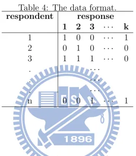
1. To analyze your own data, the form of the data must be saved as the following format in Excel:

Table 4: The data format. respondent response 1 2 3 · · · k 1 1 0 0 · · · 1 2 0 1 0 · · · 0 3 1 1 1 · · · 0 . · · · . · · · . · · · n 0 0 1 · · · 1 • Note:

(i) In the table, rows denote the numbers of respondents, and columns denote the numbers of responses. The notation 0 in Table B.1 denotes that the responses isn’t chosen and the notation 1 denotes that the response is chosen.

(ii) The data must be saved in .csv format. For example, data.csv . 2. How to run the R-codes

(i) Open R .

3. Read the data file and rank the data.

• Note: First you have to change the directory to the directory your data file saved.

(i) Read the data you want to analyze. For example, type data=read.csv(’data.csv’)

(ii) Then use the function ”ranking” to rank all the responses. For example, type ranking(data,0.05) , where 0.05 denotes the type I error of the hypothesis testing used for the raking.

• Note: In the function ranking(data,alpha), where alpha can be set by yourself.

Appendix

C

R-codes

ranking=function(data,alpha){ data=as.matrix(data) n=length(data[,1]) k=length(data[1,]) m=matrix(0,k,k) for(i in 1:k) { for(j in 1:k) { if(i==j) {m[i,j]=sum(data[,j])} if(i!=j) {m[i,j]=length(which(data[,i]==1&data[,j]==1))} } } p=matrix(0,k,k) for(i in 1:k) { for(j in 1:k) { if(i==j) p[i,j]=m[i,j]/n if(i!=j) p[i,j]=m[i,j]/n } } x=rep(0,k) for(i in 1:k) { x[i]=p[i,i] } pi=cbind(x) names(pi)=c(1:k) r=rank(pi) W=matrix(0,k,k) for(i in 1:k) { for(j in 1:k) { if(i==j) W[i,j]=0 if(i<j) W[i,j]=(p[i,i]-p[j,j])*sqrt(n/((p[i,i]-p[i,j])*(1-p[i,i]+2*p[j,j]-p[i,j])+(p[j,j]-p[i,j])*(1-p[j,j]+p[i,j]))) if(i>j) W[i,j]=-W[j,i] } } d=rep(0,k) for(i in 1:k) { d[i]=which(r==i) } z=qnorm(1-alpha/2) i=k j=k-1 g=k if(W[d[i],d[j]]>=z||W[d[i],d[j]]<=(-z))

{ r[d[k]]=1 r[d[k-1]]=2 t=r[d[k-1]] }else{ r[d[k]]=1 r[d[k-1]]=1 t=r[d[k-1]] } while((k-2)>=1) { if(r[d[k-1]]!=r[d[k]]) { i=k-1 j=j-1 if(W[d[i],d[j]]<=(-z)||W[d[i],d[j]]>=z) { r[d[k-2]]=t+1 t=r[d[k-2]] k=k-1 }else{ r[d[k-2]]=t t=r[d[k-2]] k=k-1 g=i } }else{ i=g j=j-1 if(W[d[i],d[j]]<=(-z)||W[d[i],d[j]]>=z) { r[d[k-2]]=t+1 t=r[d[k-2]] k=k-1 }else{ r[d[k-2]]=t t=r[d[k-2]] k=k-1 g=i } } } r }

Reference

[1] Agresti, A. and Liu, I.-M. (1999) Modeling a categorical variable allowing arbitrarily many category choices. Biometrics 55, 936-943.

[2] Bilder, C. R., Loughin, T. M.and Nettleton, D. (2000) Multiple marginal indepen-dence testing for pick any/c variables. Communications in Statistics-Simulation and Computation, 29(4), 1285-1316.

[3] Decady, Y. J. and Thomas, D. H. (2000). A simple test of association for contingency tables with multiple column responses. Biometrics 56, 893-896.

[4] Loughin, T. M. and Scherer, P. N. (1998). Testing for association in contingency tables with multiple column responses. Biometrics 54, 630-637.

[5] Umesh, U. N. (1995). Predicting nominal variable relationships with multiple re-sponses. Journal of Forecasting 14, 585-596.

[6] Benjamini, Y., Hochberg, Y. (1995). Controlling the false discovery rates: a practi-cal and powerful approach to multiple testing. Journal of the Royal Statistipracti-cal. B (57), 289-300.

[7] Wang, H. (2008). Ranking responses in multiple-choice questions. Journal of Ap-plied Statistics, 35, 465-474

[8] Wang, H., Chang, S. Y. (2010). Bayesian ranking responses in multiple-choice questions.