深度資訊失真對3D合成視訊的影響及品質評估

國 立 交 通 大 學

電子工程學系 電子研究所碩士班

碩 士 論 文

深度資訊失真對 3D 合成

視訊的影響及品質評估

Quality Assessment of Synthesized 3D

Video with Distorted Depth Maps

研 究 生: 劉欣哲

指導教授: 杭學鳴 教授

深度資訊失真對 3D 合成視訊的影響及品質評估

Quality Assessment of Synthesized 3D Video with

Distorted Depth Maps

研 究 生: 劉欣哲 Student: Hsin-Che Liu

指導教授: 杭學鳴 教授 Advisor: Prof. Hsueh-Ming Hang

國 立 交 通 大 學

電子工程學系 電子研究所碩士班

碩 士 論 文

A Thesis

Submitted to Department of Electronics Engineering and Institute of Electronics

College of Electrical and Computer Engineering National Chiao Tung University

In Partial Fulfillment of the Requirements for the Degree of

Master of Science in

Electronics Engineering

July 2014

Hsinchu, Taiwan, Republic of China

I

深度資訊失真對 3D 合成視訊的影響及品質評估

研究生 : 劉欣哲

指導教授 : 杭學鳴 教授

國立交通大學

電子工程學系 電子研究所碩士班

摘要

在虛擬視角的 3D 視訊編碼系統中，彩色影像和深度圖都會被壓縮並且傳送 到接收端，深度圖在壓縮的過程中會被破壞，進而導致合成視訊上也出現明顯的 失真，我們想要研究壓縮後的深度圖對合成視訊的影響，並開發出有效的品質測 定模型去估計合成視訊的品質。 我們使用 ITU/ISO 國際視訊標準 HEVC 測試模型(HTM)來壓縮深度圖，錯 誤的深度值會在物體的邊緣造成鬼影並且使物體產生不自然移動，因此，我們提 出一種新的 3D 品質估計模型，去估計因為深度圖的錯誤而對 3D 合成視訊的影 響。在我們的品質估計模型中，我們使用 SSIM 來計算圖像的基本分數，再利用 影像上的特徵(邊緣、速度及深度資訊)去計算整張影像上每一個區域的比重，進 而提升該區域的敏感度，最後在使用雙眼估計模型結合左右視訊的分數，並且選 擇適當百分比的區塊去計算最後的分數。 為了評估我們的品質測定模型的效能，我們做主觀測試實驗，總共有 30 組 測試影像，這些影像的壓縮及合成使用 HEVC-3D 的標準軟體及視角合成演算法。 總計 26 未受測者對這些測試影片進行評分，從我們的實驗結果中可以看出我們 提出的模型相較於起其他現有的模型，能更有效地估計合成視訊的主觀分數。

II

Quality Assessment of Synthesized 3D

Video with Distorted Depth Maps

Student: Du-Hsiu Li

Advisor: Prof. Hsueh-Ming Hang

Department of Electrical Engineering &

Institute of Electronics

National Chiao Tung University

Abstract

In the virtual-view 3D video coding system, both the RGB image data and the depth maps are compressed and transmitted to the receivers. After compression, the depth maps are distorted and may cause visible artifacts on the synthesized video. We study the visual effect of compressed depth maps on the synthesized video and develop a quality assessment model that predicts the subjective quality.

We use the ITU/ISO international video standard HEVC Test Model (HTM) to compress the depth maps. The distorted depth values may lead to ghost artifacts around object edges and unnatural object motions on the synthesized video. Thus, we propose a new 3D quality metric to evaluate the quality of stereo video that may contain artifacts introduced by the rendering process due to depth map errors. In our proposed quality assessment (QA) model, we use SSIM to compute the basic score of stereo image pair; we extract the edge, motion, and depth features of stereo pairs and combine them to form local weights to increase the sensitivity of the noticeable regions. We use the binocular perception model to merge the scores of stereo pairs. We also select proper percentage of image blocks in the final pooling stage.

III

To evaluate the performance of our QA model, we conduct our own subject evaluation experiments. In total, over 30 video sequences were constructed using the HEVC-3D standard software including its view synthesis tool. About 26 viewers gave subjective scores on the test sequences. Our experimental data show that our model has a better match to the subjective scores when it is compared with the other existing QA metrics.

IV

誌謝

大學四年碩士兩年都是在交大求學，系上的每一位教授都很用心的教導我們， 給於我們方向，同儕之間相互砥礪，力求進步，我的家人也全心全力的支持我， 讓我完成了碩士學位。特別感謝我的指導教授─杭學鳴教授，在研究上老師會適 時的給予方向，任何對研究有幫助的課程、演講及活動都非常鼓勵我們參加，特 別是擔任電機院院長的這段時間，就算是每天都有開不完的會，做不完的公務， 每個禮拜還是會個別的和每位碩士生開會，關心研究上或是生活上有沒有困難， 並給於協助，我非常榮幸能作為老師的指導學生。 同時也感謝杭 Group 的蔡長廷、張鈞凱、劉哲瑋、馬志堯學長，在我研究的 過程中給我很多的指導和建議，及和我的同學劉育綸、陳敬昆、周靖倫、張建誠、 陳冠諭，不管是課業上或是生活上都能共同討論互相幫助，很高興能和你們在同 一個實驗室。還有感謝 Commlab 裡的每位夥伴彥凱、唯丞、佳佑、資偉、偉生、 昀楷、中威、柏佾、文郎以及所以有的學弟妹，一起生活的這幾年充滿許多沒好 的回憶，謝謝你們的陪伴。也感謝每一位參與我的主觀實驗的所有受測者，沒有 你們幫助我沒有辦法完成我的實驗。 最後我要感謝我的家人，謝謝他們的支持和鼓勵，讓我順利地完成碩士學位， 也謝謝我的朋友們，在我覺得壓力大的時候，有你們的陪伴讓我找到宣洩的出 口。 劉欣哲 民國一百零三年 於新竹

V

Contests

摘要... I Abstract ... II 誌謝... IV Contests ... V List of Figure... VIII List of Table ... XI

Chapter 1 Introduction ... 1

1.1 Introduction ... 1

1.2 Motivation and contribution ... 1

1.3 Organization of Thesis ... 2

Chapter 2 Quality Assessment ... 3

2.1 Subjective QA Methods ... 3

2.2 Objective QA Methods ... 4

2.3 Structural Similarity (SSIM) index ... 7

2.4 Evaluation of Objective Quality Assessment Models ... 8

2.5 3D Quality Assessment Database ... 10

Chapter 3 Depth coding and artifact ... 14

VI

3.2 Depth Coding ... 15

3.3 View Synthesis ... 19

3.4 Artifacts caused by erroneous depth map ... 20

Chapter 4 Subjective Evaluation Experiments ... 23

4.1 Test Sequences ... 23

4.2 Subjective Test Setup ... 27

4.3 Result of subjective experiment ... 28

Chapter 5 Computational Objective QA model ... 30

5.1 Motivation ... 30

5.2 Feature extraction... 33

5.3 Pooling ... 39

5.4 Parameters in the computational model ... 41

5.4.1 Weight of each feature ... 41

5.4.2 Percentage of blocks used in pooling... 42

5.4.3 Parameter in Binocular Perception Model ... 42

5.5 Performance comparison ... 45

Chapter 6 CONCLUSIONS AND FUTURE WORK ... 49

6.1 CONCLUSIONS... 49

VII

VIII

List of Figure

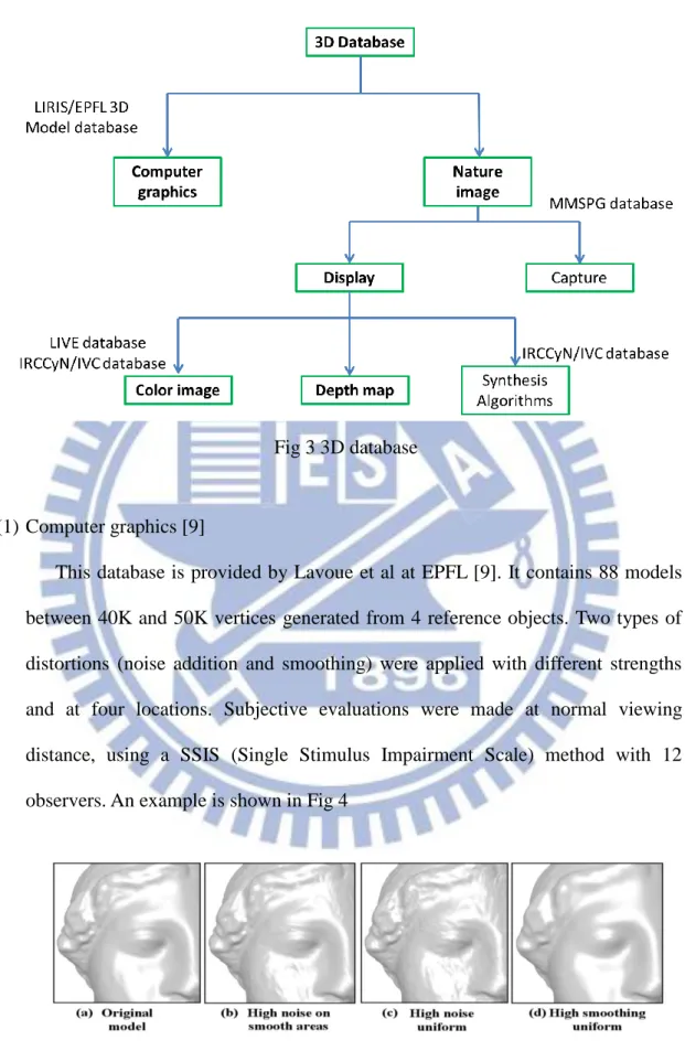
Fig 1 The structure of the Double Stimulus Continuous impairment Scale... 4

Fig 2 (a) Full-reference (b) Reduced-reference (c) No-reference ... 5

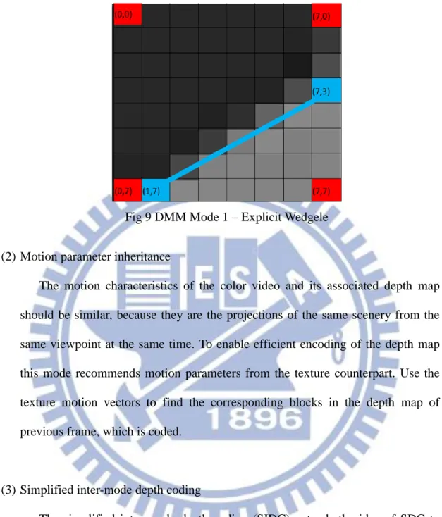
Fig 3 3D database ... 11

Fig 4 An example used in the database of computer graphics [9] ... 11

Fig 5 Six scenes used in the database [10] ... 12

Fig 6 Picture produced by different DIBR-based synthesizing algorithms [14] ... 13

Fig 7 Framework of 3DVC system ... 14

Fig 8 Planar Mode ... 16

Fig 9 DMM Mode 1 – Explicit Wedgele ... 17

Fig 10 Texture partitions and their corresponding possible depth partitions [15] .. 18

Fig 11 Illustration of 3D image warping ... 19

Fig 12 (a) Correct depth (b) Erroneous depth (c) Combine (a) and (b). ... 21

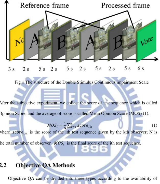
Fig 13 (a) Reference image (b) Reference depth (c) Distorted depth, and (d) Synthesized image. ... 21

Fig 14 (a) previous frame (b) present frame (c) Combine (a) and (b). ... 22

Fig 15 (a) Balloons (b) Kendo (c) Lovebird (d) Newspaper ... 23

Fig 16 The order from upper left to lower left is reference, QP 16,... 25

IX

Fig 18 The flow chart to produce the reference video ... 26

Fig 19 The environment of the subjective experiment ... 27

Fig 20 Results of subjective experiment ... 28

Fig 21 The regions that observers feel annoying ... 29

Fig 22 Examples of significant shift artifacts. (a)(c) reference and (b)(d) synthesized images... 30

Fig 23 The example of unobvious shift artifact. (a)reference (b) synthesized images ... 31

Fig 24 The example of obvious artifact: (a)reference and (b) synthesized images 32 Fig 25 The flow chart of our model ... 33

Fig 26 The result after edge detection of sequence “Street” ... 34

Fig 27 Two different search paths of 4SS. ... 35

Fig 28 The result of motion estimation of sequence “Street” ... 35

Fig 29 The example of the ghost and afterimage issues ... 36

Fig 30 The relationship between disparity and depth. ... 38

Fig 31 The disparity map of sequence “Street”... 39

Fig 32 Different value of the pooling proportion P ... 42

Fig 33 k against PLCC (P=5, n=1) for the provided model 1 ... 43

X

Fig 35 k against PLCC (P=5, n=1~7) for the provided model 2 ... 44 Fig 36 Scatter plots of the QA quality scores against the MOS using our own

database ... 46

Fig 37 Scatter plots of objective quality scores against DMOS on

XI

List of Table

Table 1 the view number used in the experiment ... 23

Table 2 QP and the corresponding QP step used in the experiment ... 24

Table 3 the quantization stepsize of the QP 0~5 ... 24

Table 4 SSIM of the original video and synthesized reference ... 26

Table 5 the performance of various metrics (our database) ... 45

1

Chapter 1 Introduction

1.1 Introduction

As the 3D display is becoming popular recently, the technology of 3D video compression plays an important role in multimedia applications. The ISO/IEC Moving Picture Expert Group (MPEG) is in the process of defining the 3D video coding (3DVC) standard that specifies the multi-view plus depth (MVD) format. Many new factors and artifacts are introduced in the new 3D video coding format. Although video quality metrics have been studied for decades, a new metrics may be need to predict the quality of the stereo images and videos.

In last decade, the development of 2D quality assessment metrics is became mature. Many well-known metrics, such as Peak Signal to Noise Ratio (PSNR), Structural Similarity (SSIM), Visual Information Fidelity (VIF) are widely used in the multimedia applications. Because the stereo images and videos are more complex than 2D, these metrics can not meet the demands of 3D context. The 3D quality assessment (QA) metrics are necessary and have room for further study.

1.2 Motivation and contribution

In a virtual-view 3D video coding system, both the RGB image data and the depth maps are compressed and transmitted to the receivers. The depth maps are distorted by the compression and the error of depth map cause the object shift (ghost artifact) and unnatural motion in the specific regions on the synthesized video after Depth Image Based Rendering (DIBR). These artifacts are different from the 2D distortions. Hence, the 2D quality assessment metrics are not sufficient to evaluate the

2

quality of synthesized video. We observe the causes of these artifacts, and propose a new quality assessment metric to predict the quality of the distorted video synthesized using the compressed depth maps. In this metric, we design the local weight of the specific regions where the artifacts are visible and include the depth information and the effect of binocular vision. We also conduct subjective viewing experiments to generate the data for our purpose. Finally, the experimental results show the our method has the higher correlation than the conventional metrics.

1.3 Organization of Thesis

We first introduce the general concepts and exiting quality assessment methods in chapter 2. We analyze the effect of the depth errors and the sources of compress depth map distortion in chapter 3. We describe our subject experiments and the experimental results in chapter 4. The proposed computational metric and its performance are shown in chapter 5. Chapter 6 is the conclusion and future work.

3

Chapter 2 Quality Assessment

Quality Assessment falls into two classes: subjective and objective quality assessment. Subjective quality assessment means that human observers watch the test video sequences and give the scores of the test sequences. Although this method is closest to the Human Visual System (HVS) but it costs man power and time to measure. The goal of objective quality assessment is to simulate HVS and judge the quality of sequence using computing algorithms. It has the advantage of lower cost for subjective quality assessment and it can be incorporated into an automatic image process system.

2.1 Subjective QA Methods

The recommendation document ITU-R BT.500 [1] describes several methods for the assessment of the picture quality. There are double-stimulus impairment scale (DSIS) method, double-stimulus continuous quality-scale (DSCQS) method, single-stimulus (SS) methods, single stimulus continuous quality evaluation (SSCQE) etc. We only describe the details of the method we use in this paper.

We use DSIS to be our experiment method, shown in Fig 1. First, the trail number is displayed for 3 seconds in the front of a sequence. Them, an image of black background with letter ‘A’ stays 2 seconds. It indicates that the coming video is the reference (stimulus A). The time of each video is about 5 seconds. Then, a leading image with letter ‘B’ is shown for the test video, which also stays 2 seconds. Then, the test video is shown for 5 seconds as stimulus B. Then, there is a 6 seconds break for the observers to vote (mark the score). In total, it takes about 37 seconds to rate one test video. In this method, we assume the reference video is perfect, and viewer gives the scores to the test video by comparing it with the reference video.

4

After the subjective experiment, we collect the score of test sequence which is called Opinion Score, and the average of score is called Mean Opinion Score (MOS) (1).

∑ (1) where is the score of the ith test sequence given by the kth observer; N is the total number of observer. is the final score of the ith test sequence.

2.2 Objective QA Methods

Objective QA can be divided into three types according to the availability of original images and videos [2]. There are shown in Fig 2.

(1). Full-reference (FR):

Most of the QA models belong to this category. And they assume undistorted reference sequence is available. Compare the undistorted and distorted sequences to estimate the quality.

5

(2). Reduced-reference (RR):

Compare to the Full-reference, this approach does not need to get the full undistorted reference sequence. They only have some feature extracting from the undistorted sequence and predict the quality of distorted sequence.

(3). No-reference (NR):

For certain applications, we can not get the undistorted reference sequence. We only can use the distorted sequences to predict the score of videos.

The Full and Reduced reference approaches also can further classify into three categories: Traditional point-based metrics, Natural Visual Characteristics and Perceptual (HVS). We explain the details blow.

(a)

(b)

(c)

Fig 2 (a) Full-reference (b) Reduced-reference (c) No-reference (a)

6

(1) Traditional point-based metrics

Mean squared error (MSE) and Peak signal-to-noise ratio (PSNR) belong to this category. Compare to other metric, they have lower computational complexity and acceptable performance. They are usually used as a part of the other metrics. (2) Natural Visual Characteristics

We first find some features or phenomena, which human pay attention to, and then predict the quality of sequence based on these feature values. It can be further classified into Natural Visual Statistics and Natural Visual Features based methods.

(A). Natural Visual Statistics

Use mean, variance, covariance, and distributions as features to predict the quality. Some famous examples are the Structural Similarity (SSIM) index [3] and the Visual Information Fidelity (VIF) [4].

(B). Natural Visual Features

Extract the obvious visual features and artifacts, like edge and blocking, and quantify their effects to predict the quality. A famous example is the Video Quality Metric (VQM) [5].

(3) Perceptual (HVS)

In this category, we develop the metrics bases on Human Visual System (HVS) characteristics. By imitating the image formative process of human to obtain the similar information transferring to brain and finally judge the quality. These metric can be classify into frequency and pixel domains.

7

(A) Frequency domains

It has been observed that the sensitivity of human visual system at different frequency is also different. To use this property, video sequence is transformed to frequency domains, usually using DCT, wavelets, and Gabor filter banks. A well-known metric using this property is MOtion-based Video Integrity Evaluation (MOVIE) index [6].

(B) Pixel domains

A part of human visual system specially deals with image edges. Hence, edges are important to the HVS. Some metrics are designed in the pixel domain such as Perceptual Video Quality Metric (PVQM) [7].

2.3 Structural Similarity (SSIM) index

This metric is proposed by Wang et al in 2004 [3]. It uses the “structural distortion” and “structural information” to predict the image quality. The SSIM index consists of three components: luminance, contrast and structure.

The calculations of luminance, contrast and structure components are defined as follows.

The function of luminance comparison:

𝑙(𝑥 𝑦) 2𝜇𝑥𝜇𝑦+𝐶1

𝜇_𝑥2_+𝜇𝑦2_+𝐶1 (2)

The function of contrast comparison:

(𝑥 𝑦) 2𝜎𝑥𝜎𝑦+𝐶2

𝜎_𝑥2+𝜎_𝑦2+𝐶₂ (3)

The function of structure e comparison:

(𝑥 𝑦) 2𝜎𝑥𝑦+𝐶3

8

where and are the means of x and y; and are the standard deviations of x and y; is the correlation coefficient between x and y, , ₂ and are the positive parameters, which are corrective terms to avoid the denominators close to zero. The definition of , and is below.

𝑁∑ 𝑥 𝑁 (5) √_𝑁− ∑𝑁 (𝑥 − )2 (6) _𝑁∑𝑁 (𝑥 − )(𝑦 − ) (7)

The Structural SIMilarity (SSIM) index is defined as below.

SSIM(x y) [l(x y)]α_{∙ [c(x y)]}β_{∙ [s(x y)]}γ ₍₈₎

Where α, β and γ are positive parameters to adjust the relative importance of the three components. To reduce the complexity of computation, SSIM has a reduced formula. In this formula, α = β = γ =1 and ₂= . The reduced form of the SSIM is (9)

𝐼 ( 2𝜇𝑥𝜇𝑦+𝐶1

𝜇𝑥2+𝜇𝑦2+𝐶1) (

2𝜎𝑥𝑦+𝐶2

𝜎𝑥2+𝜎𝑦2+𝐶2) (9)

2.4 Evaluation of Objective Quality Assessment Models

After develop a new QA metric, we need to evaluate its performance. Pearson correlation coefficient (PCC), Spearman rank order correlation coefficient (SROCC), Outlier Ratio (OR) and Root Mean Square Error (RMSE) are more commonly used. Generally, the relationship between the subjective MOS and the objective predictive scores is nonlinear.

To remove the effect of nonlinear relationship on computing the correlation coefficient, the Video Quality Experts Group (VQEG) Full Reference Television

9

(FRTV) Phase II report [8] recommends a nonlinear mapping before calculating the aforementioned criterions. It uses the following formula to match the subjective MOS and the objective predictive score.

𝑝 _{+𝑒(−𝑏2(𝑠𝑐𝑜𝑟𝑒−𝑏3))}𝑏1 (10)

where score is the score predicted by the objective QA metric and _𝑝 is the final predictive score. Parameters 𝑏 , 𝑏₂ and 𝑏 are adjusted so that _𝑝 fits MOS best. Then, use the _𝑝 and MOS to compute the PCC, SROCC, OR, RMSE. (1) Pearson correlation coefficient (PCC)

The Pearson correlation coefficient (PCC) is the linear correlation coefficient between the scores (MOS) human made and the metrics predicted. A value is closer to 1 means a better match; that is the prediction of the tested metric is more accurate. The definition is (11).

∑𝑖 1(𝑀𝑂𝑆𝑖−𝑀𝑂𝑆̅̅̅̅̅̅̅)(𝑀𝑂𝑆𝑝𝑖−𝑀𝑂𝑆̅̅̅̅̅̅̅̅)𝑝 √∑𝑖 1(𝑀𝑂𝑆𝑖−𝑀𝑂𝑆̅̅̅̅̅̅̅)2√∑𝑖 1(𝑀𝑂𝑆𝑝𝑖−𝑀𝑂𝑆̅̅̅̅̅̅̅̅)𝑝 2

(11)

where is the subjective MOS of the ith test sequence, 𝑝 is the

predictive score of the ith test sequence, n is total number of test sequence, and 𝑥̅ 𝑦̅ are the averages of 𝑥 and 𝑦, respectively.

(2) Spearman rank order correlation coefficient (SROCC)

Although the formula of SROCC is similar to that of PCC, the data pairs is different. In SROCC, the data MOS MOS need to be converted to corresponding ranks . The formula of SROCC is (12).

∑𝑖 1( 𝑖− ̅𝑖)( − ̅𝑖) √∑𝑖 1( 𝑖− ̅𝑖)2√∑𝑖 1( 𝑖− ̅𝑖)2

(12)

10

(3) Outlier Ratio (OR)

The definition of outlier ratio (OR) is the percentage of the number of difference between the subjective results and the objective score larger than 2 times the standard deviations. An OR value closer to 0 means the higher consistency of the tested metric. The definition of OR is (13).

𝑛𝑢𝑚𝑏𝑒𝑟 𝑜𝑓 𝑜𝑢𝑡𝑙 𝑒𝑟_{𝑛𝑢𝑚𝑏𝑒𝑟 𝑜𝑓 𝑑𝑎𝑡𝑎} (13)

(4) Root Mean Square Error (RMSE)

RMSE measures the accuracy of the tested metric. The definition of OR is (14). 𝐸 √_𝑛∑𝑛 ( − _𝑝 )2

(14)

2.5 3D Quality Assessment Database

In recent years, several research groups studied the 3D quality assessment topic and some of them provide their database to the public on the website. These databases contain the reference videos and the test videos with their corresponding subjective scores. These databases help the other researchers on this field to conduct the subjective experiments. For different purposes of the 3D QA research, these databases can be classified into a few categories, as shown in Fig 3.

11

(1) Computer graphics [9]

This database is provided by Lavoue et al at EPFL [9]. It contains 88 models between 40K and 50K vertices generated from 4 reference objects. Two types of distortions (noise addition and smoothing) were applied with different strengths and at four locations. Subjective evaluations were made at normal viewing distance, using a SSIS (Single Stimulus Impairment Scale) method with 12 observers. An example is shown in Fig 4

Fig 3 3D database

12

(2) Captured 3D Images [10]

This database is provided by Goldmann et al at EPFL [10]. The proposed database contains the stereoscopic videos with a resolution of 1920x1080 pixels and a frame rate of 25 fps. There are 6 scenes containing various indoor and outdoor scenes with a large variety of colors, textures, moving objects and depth structures. Each of the scenes has been captured with a static camera and different camera distances in the range 10-50 cm. It uses the single stimulus (SS) method to collect the date with 20 subjects. As example is shown in Fig 5.

(3) 3D Image with Color Distortion [11][12][13]

The first database is provided by Benoit et al in IRCCyN/IVC [11]. Six different stereoscopic images are included in this database and 15 distorted versions of each sources were generated from three different processes (JPEG, JPEG2000, blurring) symmetrically to the stereo-pair images. The second database is provided by Urvoy et al in IRCCyN/IVC [12]. Ten different stereoscopic videos are included in this database and their distorted versions are generated by H.264 and JPEG2000 coding and down-sampling and image

13

sharpening processes. The last database is provided by Moorthy et al in LIVE [13]. The database consists of 20 reference images and 365 distorted images (80 image were generated by JP2K, JPEG, white Gaussian noise and Fast-fading; 45 for were produced by Blur).

(4) Synthesis Algorithms [14]

This database is provided by Bosc et al in IRCCyN/IVC [14].It contains video generated by 7 depth-image based rendering algorithms on frames extracted from 3 video sequences. A example of synthesized images are shown in Fig 6.

In this thesis, we are interested in the effect of distorted depth map on the synthesized videos. Because our target is different from the previous ones, we construct our own test database which consists of six scenes. We use the test videos provided by the ITU/MPEG standardization committee for specifying the Advanced Video Coding (AVC, H.264) and High Efficiency Video Coding (HEVC, H.265) 3D standards. The depth maps are compressed by HTM (HEVC Test Model-8.0) and use the original color images and compressed depth maps to synthesis the virtual view image/video. The synthesis software is VSRS (View Synthesis Reference software 3.5).

14

Chapter 3 Depth coding and artifact

3.1 3D coding system codec

The 3D perception is often made by viewing two different views in two eyes, and then they are combined by the Human Visual System (HVS). The ISO/IEC Moving Picture Expert Group (MPEG) is in the process of specifying the 3D video coding (3DVC) standards based on the multiple-view plus depth (MVD) format. It assumes the input is a 2-view (or more views) video, and each view has its corresponding depth map, which can be captured by depth sensors or generated by a depth estimation algorithm. These color and depth images are then compressed by a 3D video coder. At the receiver, the virtual view images are generated by a view synthesis algorithm. Either the transmitted views or the synthesized views and their mixtures can be displayed on a 3D monitor. The framework of 3DVC system is showed in Fig 7.

15

3.2 Depth Coding

In the HTM depth coding process, there are four kinds of prediction modes (intra-prediction, motion parameter inheritance, simplified inter-mode depth coding and depth quadtree prediction) [15]. The depth maps are quantified and divided into coding blocks with different sizes. Each block chooses the prediction mode that has the least Rate Distortions cost (RD cost). After the quantization process, the coding blocks are divided into smaller blocks until the RD cost of the original block size is less than the sum of RD costs using the smaller blocks. Because the coding process needs to try all modes, it costs more time than the decoding process. In this section, we elaborate the details of these three coding modes. The Intra-prediction uses the Simplified Depth Coding (SDC) approach as an alternative intra coding mode. Two major intra prediction modes for SDC-coded blocks are Planar Mode (1 segments) and DMM Mode 1 (2 segments).

(1) Intra-prediction (A) Planar mode

The Planar Mode is often used in the smooth image area, where a number of pixels with similar depth values are grouped into one coding block. We send only the four depth values at each corner in the Planar Mode. Then the corner pixels (depth values) are used to interpolate the other depth values of each pixel in the block. Fig 8 shows an 8x8 example of the Planar Mode. The four corners are located at (0,0), (0,7), (7,0) and (7,7), and the other values in the block are then interpolated using these four values.

16

(B) DMM Mode 1 – Explicit Wedgele

The Mode often appears at object boundaries. A coding block containing both object and background is partitioned into two segments. The Wedgelet Mode transmits four corner values and the start and end points of the segmentation line (boundary). Then, the segment mean value is used to represent all pixels in one segment. Using the mean value to represent all pixels in a segment is imprecise. Therefore, the residual values between the original depth and the mean is compensated using a Depth Lookup Table (DLT). Fig 9 shows the four corners (0,0), (0,7), (7,0), (7,7), and the start and end point of the segment line (1,7) and (7,3) in the Wedgelet Mode. The mean value of segment 1 (dark color) is the mean value of (0,0), (0,7) and (7,0). And the mean value of segment 2 (light color) is the depth value of (7,7).

17

(2) Motion parameter inheritance

The motion characteristics of the color video and its associated depth map should be similar, because they are the projections of the same scenery from the same viewpoint at the same time. To enable efficient encoding of the depth map this mode recommends motion parameters from the texture counterpart. Use the texture motion vectors to find the corresponding blocks in the depth map of previous frame, which is coded.

(3) Simplified inter-mode depth coding

The simplified inter-mode depth coding (SIDC) extends the idea of SDC to inter mode depth coding. It provides an alternative residual coding method. It only encodes one DC residual value for a coding block and uses the DC residual value as residual for all value in the coding block. The DC residual of a coding block is calculated as the average of the differences between the original value and the prediction value of all pixels with the coding block.

18

(4) Depth quadtree prediction

The depth quadtree prediction mode performs a prediction of the depth quadtree from the color image quadtree. The partitioning of the depth map is limited to the same level texture partition. Hence, a given coding block of the depth map can not be split further than its collocated coding block in the texture. The possible depth partitions with their corresponding texture partition is sown in Fig 10.

19

3.3 View Synthesis

In View Synthesis system [16], the 3D image warping technique is usedto render the synthetic image with two or more contexts and depth maps of two or more different viewpoints. Use the information of camera, such as camera parameter and position, to projects the original view image object into the 3D space. Then, these image object in the 3D space are projected to the image plane of the virtual view. Fig 11 shows this projection.

is the position of image points in the original image plane. 2 is the

corresponding position of image points in the virtual image plane. and ₂ are projected to the same position in the 3D space.

𝜆 𝐾 [ 𝑍] − 𝐾 (15) 𝜆2 2 𝐾2 2[ 𝑍] − 𝐾2 2 2 (16)

where 𝜆 , 𝜆2 are the homogeneous scaling factors, 𝐾 , 𝐾2 are the 3x3 intrinsic

20

parameter matrix of the corresponding camera, , ₂ are the rotation matrixes. ,

2 are the coordinates of the camera center, and [ 𝑍]𝑇 is the corresponding

position in 3D space, which represents .

[ 𝑍

] (𝐾 )− _{(𝜆 + 𝐾 ) (17)}

Merging (16) and (17), we find the relation between and ₂.

𝜆2 2 (𝐾2 2)(𝐾 )− (𝜆 + 𝐾 ) − 𝐾2 2 2 (18)

In this thesis, we use the Fast 1-D View Synthesis, which is a part of the HEVC-based 3DV software.

3.4 Artifacts caused by erroneous depth map

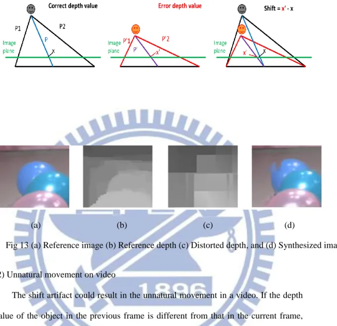
(1) Shift on image

Because the image pixels may be warped to wrong positions in view synthesis due to incorrect depth valued, the pixels shifting phenomenon appears in viewing. As shown in Fig 12(a), P1 and P2 represent the projection paths of the same object into camera 1 and camera 2. P is the projection path to the virtual camera. They all have the same depth values assuming all the cameras are in parallel. If the depth values of and ₂ are smaller than their original values due to coding errors, then Fig 12(b) shows that object is closer to the virtual camera. That is, on the image plane, the object location x is changed to location x’. The difference between

x and x’ results in the shift artifact, as illustrated by Fig 12(c). An example of this

21

(2) Unnatural movement on video

The shift artifact could result in the unnatural movement in a video. If the depth value of the object in the previous frame is different from that in the current frame, the object positions on the image plane are then shifted. In subjective viewing, the object seems to move forward or backward, as shown in Fig 14. This effect is most noticeable on the moving objects, because the foreground objects moving into or out the coding blocks may cause large changes in depth values. Because coding errors are not consistent in sign and magnitudes between nearby temporal frames, the same object may have different depth values between two frames.

(a) (b) (c) Fig 12 (a) Correct depth (b) Erroneous depth (c) Combine (a) and (b).

(a) (b) (c) (d)

22

(a) (b) (c) Fig 14 (a) previous frame (b) present frame (c) Combine (a) and (b).

23

Chapter 4 Subjective Evaluation Experiments

4.1 Test Sequences

In our experiments, we focus on the effect of distorted depth maps. We only compress the depth maps and use the original color images to synthesis the virtual images. To reduce the effect of imperfect synthesis algorithms, the reference videos are produced also by the same synthesis algorithm using the original depth maps. In our subjective quality evaluation experiments, we use six multi-view sequences (with depth maps) provided by JCT-3V Committee for the 3DVC contests. Fig 15 shows all the sequences we used and the Table 1 shows the view we use for each sequence. Four sequences have the 1024 x 768 resolution: Balloons, Kendo, Lovebird, Newspaper, and two sequences have the 1920x1088 resolution: Undo and Street.

Table 1 the view number used in the experiment

Sequence Balloons Kendo Lovebird Newspaper undo stress

View 3, 4 3, 4 6, 7 4, 5 5, 7 3.5, 4

Fig 15 (a) Balloons (b) Kendo (c) Lovebird (d) Newspaper (e) Undo (f) Stress

24

The distortion is produced 3D-HEVC test model (HTM) 8.0. We tried 5 different quantization parameters: QP=16, 27, 36, 43, 48 (Table 2).

Table 2 QP and the corresponding QP step used in the experiment

QP 16 27 36 43 48

Q_ste 4 14 40 88 160

First, we choose the best and worst quantization parameters, and then select the 3 middle values between the best and the worst. The standard specifies the relationship between QP and true quantization stepsize by the following formula.

𝑄_{𝑠𝑡𝑒𝑝}(𝑄 ) 𝑄_{𝑠𝑡𝑒𝑝}(𝑄 %6) × 2𝑓𝑙𝑜𝑜𝑟(𝑄𝑃/6) ₍₁₉₎

Table 3 the quantization stepsize of the QP 0~5

QP 0 1 2 3 4 5

Quantization Stepsize

0.625 0.6875 0.8125 0.875 1 1.125

The QP is the integer in the range 0~51 and increase of 6 means an increase of quantization step size by exactly a factor of 2.Table 3 is the first 6 values of QP with their corresponding quantization stepsizes. In this thesis, we focus on the symmetric-stereo, so the left view and the right view depth maps are compressed using the same QP and both videos are synthesized using the same view synthesis process. The depth maps compressed with 5 value are shown in Fig 16.

25

To product the test video, we compress the original stereo videos containing the color videos and depth videos. Because we want to examine the effect of the incorrect depth values on the synthesis video, we use the compressed depth maps and the original color videos to synthesize the test video. To reduce the effect of VSRS, the reference video is produced by VSRS with the original color video and the original depth map. The flow chart to produce the test video and the reference video is showed in Fig 17 and Fig 18.

Fig 16 The order fromupper left to lower left is reference, QP 16,

26

Table 4 SSIM of the original video and synthesized reference

Sequence Balloons Kendo Lovebird Newspaper undo stress

SSIM 0.954188 0.962661 0.921938 0.893475 0.976188 0.927036

The adopted virtual view synthesis algorithm is the “VSRS-1D-Fast” implemented in HTM version 3.5, which is an HEVC based reference software developed by the ITU/MPEG 3DV group.

Fig 17 The flow chart to produce the test video

27

4.2 Subjective Test Setup

In our stereo video experiments, we use Toshiba 47TL515U 47-inch 3D television. This monitor projects two images to the screen through different polarization filters and the polarizing glasses are needed to see 3D images. The viewing distance is about six times of the image height. The experimental setup is shown in Fig 19.

Our experiment contains 36 test videos, including 30 true test sequences and 6 dummy sequences. The dummy sequences are repeating the reference sequences (no distortion). The dummy sequences are inserted to judge the data consistency of a subject (observer). If the score of dummy sequences is very low, that subject (observer) data are not included. Thus, some viewing data are eliminated to make the mean opinion score (MOS) more reliable. The order of the test sequences is randomly displayed to reduce the effect of the sequence order. The duration of the entire experiment for one viewer must be less than 30 minutes. If the time is too long, the

28

observer may get tired and loose attention on watching video. Three or fewer subjects can do the experiment at the same.

4.3 Result of subjective experiment

Twenty-six observers (19 man/7 woman) with an average age of 22.6 participated in our subjective video quality evaluation. The Mean Opinion Score (MOS) of each video at various QP value is shown in Fig 20.

The difference between the reference video and test video is small for the first three QP values in most sequences. As discussed earlier, certain minor artifacts are less visible in motion video but may be noticeable in still images. However, when the QP values are sufficiently large, the depth quantization errors are high. Particularly, the object shift relative to its nearby background becomes visible. Then, the 3D visual quality drops significantly.

29

At the end of the subjective quality evaluation experiment, we asked the observers to cycle the image regions they think annoying. These data may help us to construct a computing model of 3D quality assessment. The results are shown in Fig 21. Most of these regions have moving objects and they are located at the boundaries of the foreground and the background. This is what we expect.

30

Chapter 5 Computational Objective QA model

5.1 Motivation

We first examine the conventional 2D QA models. How do they perform on 3D videos? We apply SSIM to predict the quality of stereo video. We check the SSIM map on the annoying region. The SSIM can easily detect the region of the shift artifacts. An example can be found in Fig 22.

(a) (b)

(c) (d)

Fig 22 Examples of significant shift artifacts. (a)(c) reference and (b) (d)synthesized images

31

However, not all shift artifacts can be detected by human. An example can be found in Fig 23.

Fig 23 (c) is the SSIM distribution on the test image. Clearly, the shift artifacts are detected by SSIM, but they are hard to be observed by human. These regions have heavily distorted depth maps. However, these texture regions are smooth, and the shift artifacts are less noticeable to the human. On the other hand, the SSIM is calculated pixel-by-pixel, and they are sensitive to object shifts. Thus, we use the edge information as one of our features.

Fig 23 The example of unobvious shift artifact. (a)reference (b) synthesized images (c) the SSIM map of (a) and (b)

32

In addition to the above two cases, there are other cases that the artifacts are less noticeable. For example, people pay less attention to the faraway background, as shown in Fig 24. Therefore, many 3D quality assessment models also consider the depth information as an important factor. Thus, our second feature is the depth information.

The last feature of our model is motion. Because people usually pay attention to large moving objects and the unnatural movements easily get attention. We use these three features to compute the weights of each local region. So our proposed QA model is divided into two parts. The first part computes the SSIM of the stereo video, and the second one is generating weightings based on the three extracted features of video. The proposed method computes the score of each frame and combines all frame scores to represent the score of the entire video. For each frame, we divide an image into 8-by-8 blocks, and the Structural Similarity (SSIM) metric and the feature

(a) (b)

Fig 24 The example of obvious artifact: (a)reference and (b) synthesized images

33

extraction are computed inside these 8-by-8 blocks. We then combine the scores of right and left views into the score of a frame. The flow chart of our proposed model is shown below.

5.2 Feature extraction

(1) Edge factor

Edge factor is extracting by the “Sobel” edge detector. Each edge(x,y) is assigned with value 1, if this pixel (x,y) belongs to an edge. Otherwise, its value is 0. The (u,v) pair is the index of blocks in each frame, and (x,y) is the index of pixels in a block. The equation of the edge factor is below. The result of edge detector is showed in Fig 26.

E(u v) _{8 v}∑_{(x y)∈block(u v)}e ge(x y) (20) Fig 25 The flow chart of our model

34

(2) Motion factor

The motion factor is extracted by a block matching algorithm. We use 4-Level hierarchical block matching algorithm and each level down-samples the test image by 2. The search method is the four-step search (4SS) [17] and the search area is 15-by-15. In 4SS, the first step is to find the minimum RMS from a nine-checking-points pattern on a 5-by-5 window. The second step is moving the center of the nine-checking-points pattern to the position that has the minimum RMS in the previous step. The third step is repeating step 2. The final step is similar to the step 2, but it also changes the size of the nine-checking-point pattern to 3-by-3. After step 4, the position that has the minimum RMS is the matching position. The difference between step 2 and step 3 is that step 3 is skipped if the position which has the minimum RMS in step 2 is equal to the position in step 1.

35

In Fig 27, the dots are checked in step 1, the squares are checked in step 2, the diamond-shape points are checked in step 3 and the triangles are checked in step 4. The block size is 8-by-8. The motion vector map stores the motion vector, motion(u,v) ,as shown in Fig 28 .

Fig 27 Two different search paths of 4SS.

36

We have two definitions for the motion factor and will compare their performance in section 5.5. The first definition is given below:

(𝑢 𝑣) { 0 ; 𝑖𝑓 𝑚 𝑡𝑖 𝑛(𝑢 𝑣) < 𝑚 𝑡𝑖 𝑛𝑚𝑒𝑎𝑛

𝑚𝑜𝑡 𝑜𝑛(𝑢 𝑣) ; 𝑡ℎ 𝑤𝑖 (21)

We classify the entire image into motion and non-motion regions. For each block, if the motion(u,v) is less than the threshold, it is classified as non-motion, and the motion factor is 0. Second, consider ghost and afterimage issues. When the objects move, the shift artifacts around an object look like the afterimages of that object. We can easily detect this artifact on the each frame when the video is examined frame by frame. However, this type of artifacts in the normal-speed played back video is hard to detect. Fig 29 the ghost artifact is easily detected if they are in the non-motion images.

37

In [18], they consider the effect of the camera movement on visual quality. The image may shift with a global motion and the global motion is estimated by the mean of all motion vectors in a frame. If the objects have their own motion, their motion vectors are different form the global motion vector. They classify the object motion by equation (22).

𝐼(𝑢 𝑣) { 1 ; |𝑚𝑚 𝑡𝑖 𝑛(𝑢 𝑣) − 𝑚 𝑡𝑖 𝑛𝑚𝑒𝑎𝑛| > 𝑇

0 ; 𝑡ℎ 𝑤𝑖 (22) T=Cσ, σ is the standard deviation of motion vectors in one frame, C is constant value and C is chosen 1 in their experiment. If I(u,v) equals to 1, the block is the moving object. Thus, the second definition of the motion factor is as follows.

2(𝑢 𝑣) {

0 ; |𝑚𝑚 𝑡𝑖 𝑛(𝑢 𝑣) − 𝑚 𝑡𝑖 𝑛𝑚𝑒𝑎𝑛| > 𝑇 |𝑚𝑚𝑜𝑡 𝑜𝑛(𝑢 𝑣)−𝑚𝑜𝑡 𝑜𝑛𝑚𝑒𝑎 | ; 𝑡ℎ 𝑤𝑖 (23)

38

(5) Depth information

The depth information is generated by the depth estimation methods [19]. We compute the disparity to estimate the perceptive depth value. Fig 30 illustrates the relationship between disparity and perceptive depth.

𝑑 𝑝𝑡ℎ 𝑓 ×_{𝑑 𝑠𝑝𝑎𝑟 𝑡} 𝑇 (24)

where the disparity is bigger, the object is closer. We simply use the disparity value as a disparity factor.

D(u v) isp rity(u v) (25) And the result of depth estimation is shown in Fig 31.

39

5.3 Pooling

After extracting all feature factors, we combine these three factors into a set of local weight for each frame. The weight is calculated below:

𝑤(𝑢 𝑣) 𝛼 × 𝐸(𝑢 𝑣) + 𝛽 × (𝑢 𝑣) + 𝛾 × 𝐷(𝑢 𝑣) 𝑖 ∈ {1 2} (26) We propose two models by using different definitions of motion factor. Model 1 uses the first definition of motion factor and Model 2 use the second one. The score of each block is:

(𝑢 𝑣) 1 𝑤(𝑢 𝑣)×𝑆𝑆𝐼𝑀(𝑢 𝑣) 𝑁∑(𝑢 𝑣)∈𝑖𝑡ℎ𝑓𝑟𝑎𝑚𝑒𝑤(𝑢 𝑣)

(27)

where N is the number of the total blocks.

40

To calculate the score of a stereo image pair, we incorporate the Binocular Perception Model [20] into our model. For this model, the subjective 3D image quality is

determined by the mixture of the higher and lower quality images. The equation of Binocular Perception Model is as follows:

𝑄𝑏 𝑛𝑜𝑐𝑢𝑙𝑎𝑟 {𝑘 ∙ 𝑄ℎ 𝑔ℎ𝑛 + (1 − 𝑘) ∙ 𝑄𝑙𝑜𝑤𝑛 } 1

(28) The 𝑄_{ℎ 𝑔ℎ} and 𝑄_𝑙𝑜𝑤 are the higher and lower quality of two views. We first use the right image as the basis and find the corresponding block in the left image, and then compare the block score of right view with the score of the corresponding block in left view image. Because the corresponding block may not be the original block partitioned in the first step, the position of corresponding block in left view may be between two blocks. The score of the corresponding block is interpolated using the scores of two blocks. Third, we use the binocular perception model to predict the final score of this current block.

Typical 2D QA metrics use the average score of all the pixels or blocks of the entire image to produce the final image quality index. However, in a synthesized image, the object shift and the ghost artifacts appear in specific regions due to the depth-based rendering process. Thus, we use the lowest P% of block scores instead of using all scores to calculate the frame score. After computing the scores of all frames, we compute the average score of all frames to form the final score of the test sequence.

41

5.4 Parameters in the computational model

In our computational model, there are six parameters, and we only have 30 data. The six parameters are listed below:

(1) Weights of each feature: α, β and γ

(2) The percentage of block, used in pooling :P%

(3) The parameter in the Binocular Perception Model ; w, n

5.4.1 Weight of each feature

To avoid the data over fitting, we select the α, β and γ in equation (24) to be the reciprocal of the maximum of each feature. Therefore, these three parameters are normalized to range [0 1]. However, some features can be affected by the other factors, so we add some adjustments. The motion estimation is pixel based, so the motion feature is affected by the resolution and the frame rate of sequence. To deal with this effect, we multiply the ratio of h and ℎ₀ and 𝑓 ₀ and the ratio of fr, respectively , where h is the picture height of sequence, and fr is the frame rate of sequence. In our test sequences, The ℎ₀ is set to768, and the 𝑓 ₀ is 30. The disparity weight is also pixel based, and needs to be adjusted by the sequence height, too. The final definitions of α, β and γ are as follow,

𝛼 _𝐸 𝑚𝑎𝑥 (29) 𝛽 _𝑀 𝑚𝑎𝑥× ℎ ℎ0× 𝑓𝑟0 𝑓𝑟 (30) 𝛾 _𝐷 𝑚𝑎𝑥× ℎ ℎ0 (31)

42

5.4.2 Percentage of blocks used in pooling

Fig 32 is an earlier experiment did in our lab before [21]. This experiment focused on the effect of distorted depth map on the stereo image pair. For the quantization distortion (Blue line), P is close to 5%, for the best performance. In this thesis, thus set P value to 5%.

5.4.3 Parameter in Binocular Perception Model

In equation (26), parameter k decides the weights of the higher and lower quality of two views. We decide the n and k for each provided model. If k is larger than 0.5, it means that the final score of stereo video is strongly affected by the view with the higher score. Fig 33 shows that we get the maximum performance of Model 1 when k is close to 0.84.

43

And the other parameter n is the power of the score. We try the 10 value (from 1 to 10) and the result is show in Fig 34. The PLCC achieves the maximum at n=1 for Model 1.

Fig 33 k against PLCC (P=5, n=1) for Model 1

Fig 34 n against PLCC (P=5, w=0.84) for Model 1

PLCC

k

P

LCC

44

In Fig 35, we get the maximum performance for Model 2 when k is 1. It means that the quality of stereo video is dominated by the higher quality of two views. The n value can be any number so we use n=1.

Fig 35 k against PLCC (P=5, n=1~7) for Model 2

n=1 n=2 n=3 n=4 n=5 n=6 n=7

45

5.5 Performance comparison

First we use our own database to compute the performance our computational QA model and compare this performance of our model with the four existing metrics (PSNR, SSM, MSSIM, VIF). And we use the PLCC, SROCC and RMSE to evaluate the performance of all metrics (the details of these methods are introduced in section 2.4 ) . The result is shown in Table 5 and Fig 36.

Table 5 the performance of various metrics (our database)

PLCC SROCC RMSE PSNR 0.7095 0.8173 1.4394 SSIM 0.7977 0.7641 1.5379 MSSIM 0.7751 0.767 1.6113 VIF 0.7093 0.7575 1.6510 Proposed1 0.9279 0.8441 0.7440 Proposed2 0.8142 0.7918 1.4700

The Model 1 has the best performance in our experiments. Although Model 2 has good performance too, its performance is close to that of SSIM. The matching is better when PLCC and SROCC are close to 1. On the other hand, the smaller RMSE means better matching.

46

47

We want to test our model on the other database. IRCCynN 3D [12] video quality database contains 10 sequences with 10 types of distortion. The resolution is 1920 x 1080 and the frame ratio is 25. The distortions are created by H.264, JPEG 2000 and typical image processing procedures. Although, their distorted types are different from our database, we still give a try. The result of IRCCynN database is shown in Table 6 and Fig 37.

Table 6 the performance of metric (IRCCynN database)

PLCC SROCC RMSE PSNR 0.2572 0.3499 6.0830 SSIM 0.3327 0.4630 5.9074 MSSIM 0.5680 0.5725 5.1498 VIF 0.5901 0.6242 4.6567 Proposed1 0.6175 0.6051 4.9287 Proposed2 0.6427 0.6219 4.7396

In Table 6, the proposed QA model 1 and 2 provide better results over PSNR and SSIM and are as good as MSSIM and VIF. The artifacts caused by the distorted depth maps only appear in some regions, especially in the boundary between the foreground and the background. However, JEPG 2000 and H.264 distort the color images on the entire image. In our models, the percentage of block we use to compute the score of each frame is too small for this type of distortions.

48

Fig 37 Scatter plots of objective quality scores against DMOS on the IRCCynN database

49

Chapter 6 CONCLUSIONS AND FUTURE WORK

6.1 CONCLUSIONS

In this thesis, we generate 36 test videos with distorted depth maps. These depths are compressed using the under-developed ITU/MPEG JCT-3V HEVC 3D extension standard. The purpose is to see the effect of distorted depth maps on the synthesis video. We conduct subject quality evaluation experiments on these test videos. We observe some special visual artifacts that do not occur in the conventional 3D videos that are not generated by a virtual view synthesizer. We build our 3D video subjective score database and collect the information about the annoying regions.

We also propose two computational quality assessment models to estimate the quality of distorted video synthesized by a distorted depth map. Due to two different definitions of motion factors, our model has two versions. In our proposed models, we extract edge, motion and depth features to compute the local weighting and thus enhance the effect of the “noticeable” regions with visible artifacts. Overall, we propose two new 3D video quality metrics. The experimental results indicate that the proposed methods have a higher correlation with the subjective scores (higher PLCC and lower RMSE).

6.2 Future work

In this study, we only consider the effect of distorted depth maps. In the general cases, the RGB images are also be compressed. If the RGB image and the depth map are both distorted, some new artifact may be produced. We also need to increases the test sequences to find better weights of three features. Because the time of subjective

50

experiment is limited to 30 minute, we can not do many tests in one experiment. We will need more data and then the machine learning techniques may be used to design a QA model. Furthermore, the human attention model may be included in this QA model.

51

References

[1] ITU-R Recommendation BT.500-11, “Methodology for the subjective

assessment of the quality of television pictures,” International Telecommunication

Union, Geneva, Switzerland, 2002.

[2] S. Chikkerur, V. Sundaram, M. Reisslein, and L. Karam, "Objective video quality assessment methods: A classification, review, and performance comparison,"

Broadcasting, IEEE Transactions on 57, 165 –182 (june 2011).

[3] Z. Wang, A. C. Bovik, H.R. Sheikh, and E. P. Simoncelli, “Image quality assessment: From error visibility to structural similarity,” IEEE Trans. Image Process, vol. 13, pp. 600–612, April 2004.

[4] H. R. Sheikh and A. C. Bovik, “Image information and visual quality,” IEEE

Trans. Image Process, vol. 15, no. 2, pp. 430–444, Feb. 2006.

[5] M. Pinson and S. Wolf, “A new standardized method for objectively measuring video quality,” IEEE Trans. Broadcast, vol. 50, no. 3, pp.312–322, Sep. 2004.

[6] K. Seshadrinathan and A. C. Bovik, “Motion tuned spatio-temporal quality assessment of natural videos,” IEEE Trans. Image Process, vol. 19, no. 2, pp. 335– 350, Feb. 2010.

[7] A. P. Hekstra, J. G. Beerends, D. Ledermann, F .E. de Caluwe, S. Kohler, R. H. Koenen, S. Rihs, M. Ehrsam, and D. Schlauss, “PVQM—A perceptual video quality measure,” Signal Process. Image Commun, vol. 17, no. 10, pp. 781–798, Nov. 2002. [8] Video Quality Experts Group, “Final Report from the Video Quality Experts Group on the Validation of Objective Models of Video Quality Assessment,” VQEG, August 2003.

52

driven 3D distance metrics with application to watermarking,” In proceedings of SPIE vol. 6312, 2006.

[10] L. Goldmann, F. D. Simone, and T. Ebrahimi, “Impact of acquisition distortions on the quality of stereoscopic images,” 5th International Workshop on Video

Processing and Quality Metrics for Consumer Electronics (VPQM), Scottsdale, USA,

2010.

[11] A. Benoit, P. L. Callet, P. Campisi, and R. Cousseau, “Quality assessment of stereoscopic images,” EURASIP Journal on Image and Video Processing, 2008.

[12] M. Urvoy, J. Gutierrez, M. Barkowsky, R. Cousseau, Y. Koudota, V. Ricordel, P. L. Callet, Jesús Gutiérrez and N. Garcia, “NAMA3DS1-COSPAD1:subjective video quality assessment database on coding conditions introducing freely available high quality 3D stereoscopic sequences,” Fourth International Workshop on Quality

of Multimedia Experience, Yarra Valley, July 2012.

[13] A. K. Moorthy, C,-C, Su, A. Mittal, and A.C. Bovik, “Subjective evaluation of stereoscopic image quality,” Signal Processing: Image Communication, 2012.

[14] E. Bosc, R. PéPion, P. L. Callet, M. Köppel, P. Ndjiki-Nya, M. Pressigout, and L. Morin, “Towards a new quality metric for 3-D synthesized view assessment,” IEEE

Journal on Selected Topics in Signal Processing, 2011.

[15] L. Zhang, G. Tech, K. Wegner, and S. Yea, “3D-HEVC Test Model 5,” Joint

Collaborative Team on 3D Video Coding Extensions (JCT-3V) document

JCT3V-E1005, 5th Meeting: Vienna, AT, July – Aug. 2013.

[16] C. Fehn, “Depth-image-based rending (DIBR), compression, and transmission for a new approach on 3D-TV,” in Proceedings of SPIE Stereoscopic Displays and

53

[17] L. M. Po and W. C. Ma,” A Novel Four-Step Search Algorithm for Fast Block Motion Estimation”, IEEE Trans. Circuits System, Video Technology, June 1996. [18] S. Xu, W. Lin and C.-C. J. Kuo, “Fast visual saliency map extraction from digital video,” IEEE Conference on Consumer Electronics (ICCE), Las Vegas, Nevada, USA, January 10-14, 2009

[19] E. Trucco and A. Verri, "Introductory Techniques for 3-D Computer Vision" ,

Prentice Hall, NJ, 1998, pp. 139-175

[20] D. V. Meegan, L. B. Stelmach, and W. J. Tam, “Unequal weighting of monocular inputs in binocular combination: Implications for the compression of stereoscopic imagery,” Journal of Experimental Psychology: Applied, vol. 7, pp. 143, 2001.

[21] C.-T. Tsai, “Quality Assessment of 3D Synthesized View with Depth or Color Distortion,” Masters dissertation, National Chiao Tung University, Department of Electronics Engineering2013