無線區域網路以高斯近似為基礎之變動位元速率訊務允入控制演算法

國 立 交 通 大 學

電 信 工 程 學 系 碩 士 班

碩 士 論 文

無線區域網路以高斯近似為基礎之變動位

元速率訊務允入控制演算法

Gaussian Approximation Based Admission

Control Algorithm for Variable Bit Rate Traffic

in IEEE 802.11e WLANs

研究生 ：黃郁文

指導教授：李程輝 教授

允入控制演算法

Gaussian Approximation Based Admission Control

Algorithm for Variable Bit Rate Traffic in IEEE 802.11e

WLANs

研 究 生： 黃郁文

Student: Yu-Wen Huang

指導教授： 李程輝 教授

Advisor: Prof. Tsern-Huei Lee

國 立 交 通 大 學

電 信 工 程 學 系 碩 士 班

碩 士 論 文

A Thesis

Submitted to Department of Communication Engineering College of Electrical and Computer Engineering

National Chiao Tung University in Partial Fulfillment of the Requirements

for the Degree of Master of Science

in

Communication Engineering June 2006

Hsinchu, Taiwan, Republic of China.

無線區域網路以高斯近似為基礎的變動位元速率訊務

允入控制演算法

學生: 黃郁文 指導教授: 李程輝 教授

國立交通大學電信工程學系碩士班

中文摘要

為了提供即時性訊務的服務品質保證，IEEE 802.11 標準制定團隊引入『混 合協調功能』(Hybrid Coordination Function)的通道存取機制，其中又分成兩種模 式，以競爭來獲得通道存取權利的方法稱為 Enhanced Distributed Channel Access (EDCA)；另一種則為非競爭的通道存取模式稱為 Hybrid Controlled Channel Access (HCCA)。然而，在 HCCA 排程器中，允入控制與分配傳送機會(TXOP) 的 參考設計只適用於傳送固定位元速率(CBR)的訊務，對於傳送變動位元速率(VBR) 的訊務來說，則可能會發生嚴重的封包遺失(Packet Loss)。 在這一篇論文中，我們提出了一個簡單的允入控制演算法，其基本設計的思 維在於利用高斯分佈(Gaussian Distribution)來近似變動位元速率的訊務。電腦模 擬的結果指出我們提出的允入控制演算法，可以來確保擁有服務品質保證的站台 (QoS-Enhanced Station)在傳送訊務的過程中，封包遺失的機率在事前保證的範圍 以內。再者，當有站台一次要求傳送多個變動位元速率之訊務流時，我們提出的 方法可以因為獲得多工增益(Multiplexing Gain)而更有效率的分配傳送機會 (TXOP)。

Algorithm for Variable Bit Rate Traffic in IEEE

802.11e WLANs

Student: Yu-Wen Huang Advisor: Prof. Tsern-Huei Lee

Institute of Communication Engineering

National Chiao Tung University

Abstract

For Quality of Service (QoS) requirements of real-time traffic, IEEE 802.11 working group introduces a QoS-aware channel access mechanism, called Hybrid Coordination Function (HCF), which consists of contention-based Enhanced Distributed Channel Access (EDCA) and contention-free HCF Controlled Channel Access (HCCA). The TXOP allocation and the admission control units of the HCCA reference scheduler are only appropriate for constant bit rate (CBR) flows. It may result in serious packet loss for variable bit rate (VBR) flows.

In this thesis, we propose a simple admission control algorithm which adopts Gaussian distribution to approximate VBR traffic. Numerical results obtained from computer simulations show that our proposed algorithm can effectively and efficiently allocate Transmission Opportunity (TXOP) durations to QoS-enhanced stations (QSTAs) to guarantee a predefined packet loss probability. Moreover, our proposed scheme can easily handle multiple VBR flows of the same QSTA to get the advantage of multiplexing gain.

誌謝

經歷了一番琢磨，這一篇論文終於可以定稿！首先要感謝的是我的指導教授 ─ 李程輝教授。在論文完成的過程中，李教授教導我解決問題的正確觀念和撰 寫論文的嚴謹態度，使我能夠在研究的過程中獲得寶貴的經驗和成就感。 接著要感謝 我的父母 ─ 黃吉財先生和王淑英女士。除了養育之恩以外，在成長過程 中，父親告誡我『勝而不驕，敗而不餒』的運動精神；在求學過程中，母親培養 我『積極進取』的學習態度，均成為我一生受用不盡的寶藏。 我的兄長黃乾庭先生從小的照顧與勉勵和我的女友林怡君小姐一路的支持 與陪伴，均讓我的生活因為充實而多彩多姿。 實 驗 室 的 學 長 ─ 景 融 在 研 究 過 程 中 所 給 予 的 指 導 ， 還 有 同 窗 政家、迺倫、紹瑜和學弟們在研究的路途上所給予的鼓勵，這些均豐富了我的研 究生活。 最後謹將此篇論文獻給在天上的奶奶， 您的教誨依舊深植在我心中，不曾或忘！ 黃郁文 2006 年 6 月於風城交大

Contents

中文摘要 i English Abstract ii 誌謝 iii Contents iv List of Tables vi

List of Figures vii

Acronym viii

Chapter 1 Introduction 1

Chapter 2 Background 4

2.1 Overview of IEEE 802.11 Protocol Architecture……….. 4

2.2 Distribution Coordination Function.………. 6

2.3 Point Coordination Function………. 10

2.4 Hybrid Coordination Function...………... 11

2.5 Enhanced Distributed Channel Access………... 12

2.6 HCF Controlled Channel Access………... 14

Contents

Chapter 3 Related Works 18

3.1VBR traffic with Constant Packet Size... 19

3.2 VBR traffic with Variable Packet Size... 20

Chapter 4 Gaussian Approximation Based Admission Control Algorithm 22 4.1 Motivation………... 22

4.2 Gaussian Approximated VBR traffic... 24

4.3 VBR traffic with Constant Packet Size... 25

4.4 VBR traffic with Variable Packet Size... 26

4.5 Gaussian Approximation Based Admission Control Algorithm…... 26

4.6 Aggregated TXOP Duration……….. 28

Chapter 5 Analysis of Packet Loss Probability 29 5.1 Analysis of Packet Loss Probability……….. 29

5.2 Approximation of Packet Loss Probability………... 30

Chapter 6 Simulation Results 33

Chapter 7 Conclusions 39

List of Tables

2.1 The mapping between the user priorities in 802.1D and the access

categories in IEEE 802.11e ... 12

2.2 Values for the EDCA parameter sets ... 14

2.3 TSPEC element fields ... 15

3.1 Definition of parameters shown in equation (6)………. 20

3.2 Definition of parameters shown in equation (7) and (8)……….. 21

6.1 PHY and MAC parameters……….. 34

6.2 Transmission time for different header and per-packet overhead………… 34

6.3 QoS parameter of different traffic……… 35

6.4 Simulation result for constant packet size……… 36

6.5 Simulation result for variable packet size……… 37

List of Figures

List of Figures

2.1 IEEE 802.11 Protocol Architecture... 5

2.2 MAC Architecture... 6

2.3 IEEE 802.11 Medium Access Logic…... 7

2.4 Basic access method of DCF ...………... 8

2.5 Example of hidden node problem ... 8

2.6 DCF enhanced with CTS/RTS mechanism ... 9

2.7 PCF basic operating procedure ... 10

2.8 Comparison of backoff entities between 802.11 and 802.11e ... 13

2.9 Correlations between AC and EDCA parameters ... 14

4.1 Instantaneous rate of one VBR flow……… 22

4.2 Data rate distribution for one VBR flow……….. 24

5.1 Equivalent system model………. 29

Acronym

AC access category

ADDTS add traffic stream

AIFS arbitration interframe space

BSS basic service set

CA collision avoidance

CAP controlled access phase (period)

CDF cumulative distribution function

CF-Poll contention-free polling frame

CFP contention-free period

CSMA carrier sense multiple access

CW contention window

DCF distributed coordination function

DIFS DCF interframe space

DSSS direct sequence spread spectrum

EDCA enhanced distributed channel access

HC hybrid coordinator

HCCA HCF controlled channel access

HCF hybrid coordination function

IEEE Institute of Electrical and Electronics Engineers

MAC medium access control

NAV network allocation vector

OFDM orthogonal frequency division multiplexing

PIFS PCF interframe space

PC Point Coordinator

PCF Point Coordination Function

QAP QoS enhanced access point

QoS quality of service

QSTA QoS enhanced station

SI service interval

SIFS short interframe space

TS traffic stream

TSPEC traffic specification

Chapter 1 Introduction

Chapter 1

Introduction

In recent years, real-time services have become popular Internet applications. To satisfy the Quality of Service (QoS) requirements such as guaranteed packet delay and packet loss probability has, therefore, become more and more important for the design of Medium Access Control (MAC) Protocol. The original IEEE 802.11 MAC protocol, unfortunately, does not possess any mechanism for satisfying QoS requirements of real-time applications. Therefore, a new standard, i.e., IEEE 802.11e, is proposed to enhance the QoS support in Wireless LANs.

IEEE 802.11e introduces a new coordination function which is called Hybrid Coordination Function (HCF). This function defines two channel access mechanisms: one is contention-based Enhanced Distributed Channel Access (EDCA) and the other is contention-free HCF Controlled Channel Access (HCCA).

The HCCA mechanism requires a QoS-aware Hybrid Coordinator (HC), which usually is equipped in the Access Point (AP) of infrastructure WLANs and is able to gain control of the channel after sensing the medium idle for a PCF inter-frame space (PIFS) interval. In other words, HC has a higher priority to access the medium than normal QoS-enhanced stations (QSTAs).

After gaining control of the transmission medium, HC will poll QSTAs on its polling list. In order to be included in HC’s polling list, each QSTA needs to make a

separate QoS service reservation, which is achieved by sending Add Traffic Stream (ADDTS) frame to HC. In this frame, QSTAs can give their service requirements a detailed description in”Traffic Specification” (TSPEC) field. To support the QoS requirement specified in TSPEC, HC calculates a common service interval and Transmission Opportunity (TXOP) for each flow.

Upon receiving a poll, the polled QSTA either responds with a QoS-Null frame if it has no packet to send or responds with QoS-Data frame if it has packets to send. When the TXOP duration of some QSTA ends, HC gains the control of channel again and either sends a QoS poll to the next station on its polling list or releases the medium if there is no more QSTA to be polled.

The TXOP calculation provided by the reference scheduler in IEEE 802.11e standard document is based on mean data rate and nominal MSDU size. It only fits the characteristics of CBR traffic. For VBR traffic, it may cause serious packet loss. Therefore, previous research tried to modify the TXOP computation and the admission control unit so that the packet loss probability can be controlled under a predetermined threshold. In [3], an expression of packet loss probability was defined and derived in terms of allocated TXOP duration. The bisection method is adopted to calculate the Effective TXOP duration with guaranteed packet loss probability. Since the exact probability distribution function of packet arrival is used in the expression, the TXOP calculation was shown to be accurate. However, the computational complexity of the bisection method could make the scheme infeasible in practice. Moreover, the expression is only for a single traffic flow, meaning that the algorithm does not take advantage of multiplexing gain when there are multiple VBR flows in the same QSTA.

Chapter 1 Introduction

In this thesis, we use Gaussian distribution to approximate the behavior of VBR traffic. As a result, it is much easier to calculate the Effective TXOP durations than using the bisection method. The proposed algorithm requires only the first two moments of packet arrival, instead of the exact distributions. Besides, multiplexing gain can be easily obtained because the calculation is basically the same when there are multiple VBR traffic flows in the same QSTA.

The remainder of this paper is organized as follows. In Chapter 2, the legacy MAC mechanism in IEEE 802.11 and the enhanced one in IEEE 802.11e are described. After a survey of related work about admission control for IEEE 802.11e in Chapter 3. Chapter 4 and Chapter 5 respectively present our proposed algorithm and analysis of packet loss probability while input is Gaussian process. Chapter 6 shows the performance evaluation of our proposed algorithm. Finally, we draw our conclusions and future work in Chapter 7.

Chapter2

Backgrounds

As the name suggests, Wireless LAN is one that exploits the wireless medium for transmission. Compared to traditional wired systems, this technology extends the area that people can access Internet or some other information. As a result, it was deployed rapidly and widely in our life.

In 1999, IEEE working group defines a standard of Wireless LANs, named IEEE 802.11. The following sections will give a clear description of IEEE 802.11.

2.1 Overview of IEEE 802.11 Protocol Architecture

IEEE 802.11 includes the specification of Physical layer and Medium Access Control (MAC) layer of Wireless LANs. Nowadays, there are various versions of IEEE 802.11, which adopts different modulation schemes and operates in different bands. Such as IEEE 802.11b, it adopts complementary code keying (CCK) and direct sequence spread spectrum (DSSS) as transmission scheme and operates in 2.4GHz industrial, scientific, and medical (ISM) band with the data rate provided up to 11Mbps. As for IEEE 802.11a, it can support the data rate up to 54Mbps with orthogonal frequency-division multiplexing (OFDM) applied and 5GHz unlicensed national information infrastructure operated. There still are other versions, which are summarized in Figure 2.1 and thus are not repeated.

Chapter 2 Backgrounds

Figure 2.1: IEEE 802.11 Protocol Architecture [10]

The MAC mechanism shown in Figure 2.1 consists of Distributed Coordination Function (DCF) and Point Coordinated Function (PCF). The design concepts of these functions are suitable for best-effort traffic. As for real time traffic which needs some service guarantees, these functions can not provide the Quality of Service (QoS). For satisfying these QoS requirements, IEEE working group defines a new specification called IEEE 802.11e. In this specification, a new coordination function is proposed, which is called Hybrid Coordination Function (HCF). This function is composed of two mechanisms: one is contention based Enhanced Distributed Coordination Function (EDCA), and the other is Hybrid Controlled Channel Access (HCCA). The relationship among the above described mechanisms is shown in Figure 2.2.

Figure 2.2: MAC Architecture [2]

The following sections focus on the individual MAC mechanism shown in Figure2.2 and give a detailed survey.

■

2.2 Distributed Coordination Function [1]

Distributed Coordinated Function (DCF) is the basic medium access mechanism in IEEE 802.11 MAC layer. The basic concept of DCF is CSMA/CA (Carrier Sense Multiple Access with collision voidance) algorithm. It works as a “listen before talk” scheme. If the station has packets to send and senses the medium is free, it will still wait for one time duration, called DIFS (DCF Inter-frame Space). After that, the station will either deliver the packets or initiate a back-off counter, depends on whether the channel is still free or not. When a back-off counter is initiated, a station will wait for the end of transmission and once the channel is free for DIFS again, the station will start the back-off procedure which refers to the decrementing of back-off

Chapter 2 Backgrounds

counter. The value of back-off counter is uniformly selected between zero and

contention window (CW) which initially equals to CWmin (minimum value of

contention window). If the back-off counter reduced to zero and the channel is still free, the station will transmit its packets. However, if the channel becomes busy in the middle of the back-off procedure, the station will freeze the back-off counter, and resumes to countdown after deferring a period, called Network Allocation Vector (NAV), which is indicated in the winning station’s packet header. The basic logic of IEEE 802.11 MAC and basic access method of DCF are shown in Figure 2.3 and Figure 2.4 respectively.

Figure 2.4: Basic access method of DCF [10]

It is possible that two or more stations transmit their packets at the same time which leads the occurrence of collision. Collisions are inferred by no Acknowledgement (ACK) from the receiver. Collision resolution process is handled by the exponential back-off procedure, which refers that whenever collisions occur, the current CW will be doubled and a valued between zero and the doubled CW will be chosen for decrement. If collisions still occur, this procedure will be executed

again until CW up to CWmax (maximum value of contention window). When a station

succeeds to transmit their packets, its CW will be reset to CWmin.

Chapter 2 Backgrounds

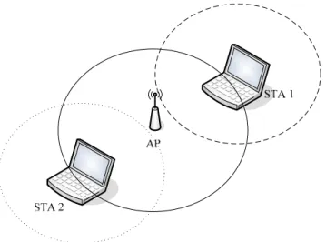
There still is one problem that the basic DCF mechanism and exponential back-off procedure can not solve, called “Hidden Terminal Problem”, an example of which is cleared shown in Figure 2.5. In this figure, STA 1 and STA2 can not detect the existence of each other. Therefore, they may be cause serious interference for AP (Access Point) to receive data. Thus, CTS/RTS mechanism is proposed to resolve this problem.

Figure 2.6: DCF enhanced with CTS/RTS mechanism [9]

The CTS/RTS mechanism works as follows. When a station decides to transmit packets, it will send RTS (Request to Send) to AP instead of delivering packet directly. After receiving RTS packet, the designated receiver will reply a CTS packet to inform the sender within its reception range to set NAV. With this mechanism, STA 1 in Figure 2.5 can sense the medium is occupied by STA 2 through CTS packet delivered by AP. Thus, “Hidden Terminal Problem“can be solved.

2.3 Point Coordination Function [1]

Compared to distributed style as DCF shown in previous section, Point Coordinate Function (PCF) introduces a centralized coordinator, called Point Coordinator (PC). Each station in PCF mode can transmit packet only when received a poll from PC. Thus, the problems in DCF such as collision, Hidden terminal, do not occur. The basic operating procedure is presented in Figure 2.7

Figure 2.7: PCF basic operating procedure [9]

With the PCF, the contention period (CP) and contention free period (CFP) alternate periodically overtime. Within CP, stations in the basic service set (BSS) will follow DCF mechanism. After a Beacon frame initiates, CFP starts and the stations in the BSS will set their NAV to the end of CFP. During CFP, there is no contention among stations; instead, stations are polled. PC will poll the stations for transmitting packets. If a polled station has packets to send, it will deliver its packets and ACK of the poll after SIFS period. When a poll packet is sent for longer than Point Inter-frame

Chapter 2 Backgrounds

Space without any reply, PC will send poll to another station or end CFP.

There are still some problems in PCF which motivates the working group to enhance the protocol. Among most of others, we can list two problems that is most obvious.

z Unpredictable Beacon Delay

z Unknown transmission durations of polled stations

For resolving these problems, IEEE 802.11e is proposed, and the following will give a clear description of its mechanisms.

■

2.4 Hybrid Coordination Function[2]

To support QoS, IEEE 802.11 working group introduces a new coordination function, called Hybrid Coordination Function (HCF). This function defines two channel access mechanisms: one is contention-based Enhanced Distributed Channel Access (EDCA) and the other is contention-free HCF Controlled Channel Access (HCCA). The following will give detailed surveys of EDCA and HCCA.

2.5 Enhanced Distributed Channel Access [2]

Enhanced Distributed Channel Access (EDCA) adopts a differentiated, distributed way to coordinate the channel access. The differentiated services are realized by classifying the packets into four access categories shown in Figure 2.8. Each access category has its own arbitration interframe space (AIFS[AC]) and minimum size of contention window. The AIFS[AC] is at least equal to DIFS and can be enlarged with the arbitration interframe space number, AIFSN[AC]. The AIFS[AC] can be defined as

(1)

[

]

[

]

,

[

]

2

AIFS AC

=

SIFS

+

AIFSN AC aSlotTime AIFSN AC

⋅

≥

.

Table 2.1: The mapping between the user priorities in 802.1D and the access categories in IEEE 802.11e [7]

Chapter 2 Backgrounds

The basic access mechanism of EDCA is basically the same as DCF. The differences are that stations enhanced with EDCA will start to count down after sensing the channel busy for AIFS[AC], and the backoff process will choose a random number between zero and the size of contention window, which has minimum size,

CWmin[AC] and maximum size, CWmax[AC] summarized in Figure 2.8. The values of

AIFS[AC], CWmin[AC], CWmax[AC] for each AC are shown in Table 2.1.

Based on the basic channel access mechanism, we can say that the smaller

AIFS[AC] and CWmin will lead to the higher probability to occupy the channel. In

other words, one access category with higher priority will be assigned smaller

AIFS[AC] and CWmin. More clear comparison will be presented on Figure 2.9.

Table 2.2: Values for the EDCA parameter sets[3]

Figure 2.9: Correlations between AC and EDCA parameters [3]

■

2.6 HCF Controlled Channel Access [2]

The HCCA mechanism requires a QoS-aware Hybrid Coordinator (HC), which usually is equipped in the Access Point (AP) of infrastructure WLANs and is able to

Chapter 2 Backgrounds

gain control of the channel after sensing the medium idle for a PCF inter-frame space (PIFS) interval. In other words, HC has a higher priority to access the medium than normal QoS-enhanced stations (QSTAs).

After gaining control of the transmission medium, HC will poll QSTAs on its polling list. In order to be included in HC’s polling list, each QSTA needs to make a separate QoS service reservation, which is achieved by sending Add Traffic Stream (ADDTS) frame to HC. In this frame, QSTAs can give their service requirements a detailed description in the ”Traffic Specification” (TSPEC) field. To support the QoS requirement specified in TSPEC, HC calculates a common service interval and Transmission Opportunity (TXOP) for each flow.

Upon receiving a poll, the polled QSTA either responds with a QoS-Null frame if it has no packet to send or responds with QoS-Data frame if it has packets to send. When the TXOP duration of some QSTA ends, HC gains the control of channel again and either sends a QoS poll to the next station on its polling list or releases the medium if there is no more QSTA to be polled.

The detailed HCCA scheduler and reference admission control unit are shown in the next section.

Element ID (13) Length (55) TS Info Nominal MSDU Size Maximum MSDU Size Minimum Service Interval Maximum Service Interval Inactivity Interval Suspension Interval Service Start Time Minimum Data Rate Mean Data Rate Peak Data Rate Maximum Burst Size Delay Bound Minimum PHY Rate Surplus Bandwidth Allowance Medium Time

2.7 The Reference HCCA Scheduler

In the reference scheduler provided in IEEE 802.11e standard document, a mandatory set of TSPEC parameters are required for QoS negotiation. This parameter set includes Mean Data Rate (ρ), Nominal MSDU size (L) and Maximum Service Interval (SImax).

In order not to violate the packet delay bounds of all admitted flows, HC chooses

a number, which is lower than the minimum of maximum service interval (SImax) for

all admitted traffic flows which is also a sub-multiple of the beacon interval as the Scheduled Service Interval (SI). In addition, HC calculates TXOP duration for each

flow by the following steps. First of all, HC decides the average number of packets Ni

that arrives at the mean data rate during one SI for a specific flow i:

(2)

⎥

⎥

⎤

⎢

⎢

⎡ ⋅

=

i i i

L

SI

N

ρ

Secondly, the TXOP duration is obtained for flow i as follows:

⎭

⎬

⎫

⎩

⎨

⎧

+

⎟⎟

⎠

⎞

⎜⎜

⎝

⎛

+

×

=

O

R

M

O

R

L

N

TD

i i i i i i

max

,

(3)

where Ri is the Minimum Physical Transmission Rate, Li and Mi are, respectively, the

Nominal Packet Size and Maximum MSDU size of flow i, and O denotes the per-packet overhead in time units. This overhead O includes the transmission time for ACK frame, inter-frame space, MAC header, CRC field and PHY PLCP Preamble and Header.

Chapter 2 Backgrounds

Finally, the total TXOP duration of station j with n traffic flows is

1 n j i i

TXOP

TD

SIFS t

=

⎛

⎞

=

_⎜

_⎟

+

+

⎝

∑

⎠

POLL (4)

where SIFS and TPOLL are, respectively, the short inter-frame space and the

transmission time of CF-Poll frame.

After calculating TXOPi, the admission control unit will admit this newly arrived

flow when the following inequality is satisfied:

∑

− =

−

≤

+

1 1 i k b cp b k i

T

T

T

SI

TXOP

SI

TXOP

(5)

where Tb and Tcp are the length of beacon interval and contention period, respectively.

If the new flow is admitted with a Maximum service interval smaller than the current

SI, the scheduler will update a new SI which can satisfy the requirement of this new

flow. Of course, the TXOP durations for all the admitted flows in the polling list need to be recalculated according to the new SI.

Chapter 3

Related Work

As described in Chapter 2, the method for allocating TXOP durations in the reference scheduler is based on the mean data rate and nominal MSDU size. It is effective for CBR traffic. For VBR flow, however, it may cause serious packet loss due to fluctuation of data rate and packet size. This chapter describes the scheme proposed in [3] which tried to provide QoS guarantee for VBR traffic.

In [3], VBR traffic is classified into two cases: constant packet size and variable packet size. The packet loss probability is defined in terms of TXOP duration (TD) for both cases. For every admitted flow of a QSTA, the allocated TXOP is fixed in each SI.

In the definition of packet loss probability, each TXOP is assumed only to serve the packets which arrived during the time interval between the beginning of the previous and current TXOP which is equal to one SI. If the allocated TXOP is not enough to transmit all the packets arrived during previous SI, the remaining packets in the queue will not be delayed to next SI. Therefore, the maximum delay is guaranteed to be lower than SI. The packet loss probability analysis and the method to calculate Effective TXOP are shown in the following.

Chapter 3 Related Work

3.1 VBR Traffic with Constant Packet Size

In the case of constant packet size, only the packet arrival rate is varying and the packet loss probability can be defined as mean packet loss over mean packet arrival during one SI. It can be represented as:

(6)

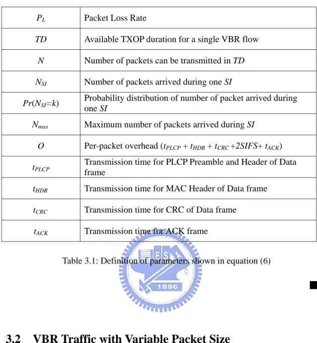
Note that NSI is the number of packets arrived during one SI and N is the number

of packets that can be transmitted in one SI. The numerator is the average of (NSI –N)

for NSI > N. Nmax is the maximum number of packets arrived during one SI which is

related to the peak rate of this flow shown in its TSPEC field. The other parameters are summarized in Table 3.1.

The Effective TXOP duration given the packet loss probability (PL) of a single

VBR flow with constant packet size can be obtained by applying bisection method to equation (6).

(

)

( )

(

) (

)

(

)

⎥

_⎥

⎤

⎢

⎢

⎡

+

=

⋅

⎟

⎠

⎞

⎜

⎝

⎛

=

−

=

−

=

∑

> +

O

R

L

TD

N

SI

L

n

N

N

n

N

E

N

N

E

P

N N n SI SI SI L

where

Pr

max

ρ

PL Packet Loss Rate

TD Available TXOP duration for a single VBR flow

N Number of packets can be transmitted in TD

NSI Number of packets arrived during one SI

Pr(NSI=k) Probability distribution of number of packet arrived during

one SI

Nmax Maximum number of packets arrived during SI

O Per-packet overhead (tPLCP + tHDR + tCRC +2SIFS+ tACK)

tPLCP

Transmission time for PLCP Preamble and Header of Data frame

tHDR Transmission time for MAC Header of Data frame

tCRC Transmission time for CRC of Data frame

tACK Transmission time for ACK frame

Table 3.1: Definition of parameters shown in equation (6)

■

3.2 VBR Traffic with Variable Packet Size

In the case of variable packet size, both packet arrival rate and packet size are varying. The packet loss probability is expressed in terms of transmission time of packets rather than the number of packets. That is, the definition is average transmission time required to transmit the lost packets over the average transmission time of packets arrived during one SI. It can be represented as the following.

Chapter 3 Related Work

(7)

(8)

Definitions of the parameters in equations (7) and (8) are summarized in Table 3.2. Detailed derivation can be found in [3]. Again, the Effective TXOP duration can be obtained by using the bisection method to equation (8) given the packet loss probability (PL).

(

)

( )

(

) ( )

( )

(

)

( ) ( )

_{( )}

( ) ( ) (

)

(

)

(

)

[

]

(

)

max 1 1 1 1 where ! 1 where 1 ! ! SI SI N SI i L SI i SI n N R TD nO n T _n TD SI n n n n i n i E T TD X P T O E T R e h t TD f t dt _n X E N E O _O R R R TD nO h TD n R TD nO n nO TD R n α λ α α λ λ λ λ + = − + − ∞ = − − = − = = + − = = ⋅ + ₊ − = − − + + − −

⎛

⎞

⎜

⎟

⎝

⎠

⎛

⎞

⎜

⎟

⎝

⎠

⎛

⎞

⎜

⎟

⎝

⎠

∑

∑

∫

∑

TD i

TSI Transmission time required for transmitting NSI packets

TD Allocated TXOP duration

Xi

Packet Size is modeled by Exponential Distribution with mean equal to Nominal packet size (L)

λ λ=1/L

α Mean packet arrival rate

Table 3.2: Definition of parameters shown in equation (7) and (8)

Chapter 4

Gaussian Approximation Based Admission Control

Algorithm

4.1 Motivation

The TXOP calculation provided by the reference scheduler in IEEE 802.11e standard document is based on mean data rate and nominal MSDU size. It only fits the characteristics of CBR traffic. For VBR traffic, it may cause serious packet loss. Figure 4.1 shows the relationship between data rate of VBR traffic and time. It is obvious that if average rate is considered, packet loss probability may out of our control.

Chapter 4 Gaussian Based Admission Control Algorithm

Therefore, the research described in Chapter 3 tried to modify the TXOP computation and the admission control unit so that the packet loss probability can be controlled under a predetermined threshold. In section 3.1 and 3.2, an expression of packet loss probability was defined and derived in terms of allocated TXOP duration. The bisection method is adopted to calculate the Effective TXOP duration with guaranteed packet loss probability. Since the exact probability distribution function of packet arrival is used in the expression, the TXOP calculation was shown to be accurate. However, the computational complexity of the bisection method could make the scheme infeasible in practice. Moreover, the expression is only for a single traffic flow, meaning that the algorithm does not take advantage of multiplexing gain when there are multiple VBR flows in the same QSTA.

We are motivated by data rate distribution of VBR traffic shown in Figure 4.2. The shape of its probability density function is similar to that of Gaussian distribution. In addition, central limit theorem shows that sum of general random variables will converge to Gaussian distribution as the number of these approaches to infinity. Therefore, using Gaussian distribution to approximate data rate distribution of VBR traffic seems to be feasible.

When this approximation is adopted, it is much easier to calculate the Effective TXOP durations than using the bisection method. Our proposed algorithm requires only the first two moments of packet arrival, instead of the exact distributions. As a result, it can be realized under low computation load. Besides, multiplexing gain can be easily obtained because the calculation is basically the same when there are

multiple VBR traffic flows in the same QSTA.

Figure 4.2: Data rate distribution for one VBR flow

■

4.2 Gaussian Approximation of VBR Traffic

In our proposed algorithm, the behavior of every single VBR traffic is approximated by Gaussian distribution. Let Y denotes the total amount of traffic arrived for a single VBR flow in one SI. We have

(9) 1 K i i

Y

X

=

=

∑

where K is the number of packets arrived in one SI and Xi is the size of the ith packet.

Chapter 4 Gaussian Based Admission Control Algorithm

According to Chapter 5 of [5], we can conclude that

(10) Since

( )

(

( )

)

( )

( )

( )

where

is moment generating function of

is moment generating function of

is probability generating function of

Y K X Y X K

M

G M

M

Y

M

X

G z

K

θ

θ

θ

θ

=

( )

_{( )}

( )

( )

_{( )}

_{( )}

_θ

θ

θ

M

d

d

M

n

Y

E

M

n n n n n

=

=

=

where

,...

3

,

2

,

1

,

0

₍₁₁₎

we get E(Y) by letting n=1,

( )

Y

E

( ) ( )

K

E

X

E

=

⋅

(12)

Similarly, by letting n=2, we can obtain E(Y2). After some simple derivations, we have

( )

( )

( )

(

( )

)

2

( )

VAR Y

=

E K VAR X

⋅

+

E X

⋅

VAR K

(13)

■

4.3 VBR Traffic with Constant Packet Size

In this case, we assume K is Poisson distributed with E(K)= λ and X is a _i

constant L for all i. Therefore, according to equations (12) and (13), the mean and variance of this traffic are given by

(14) (15) ■

( )

Y

L

E

=

λ

⋅

( )

Y

L

VAR

=

_λ

2

⋅

4.4 VBR Traffic with Variable Packet Size

In this case, we assume K is Poisson distributed with E(K) =λ and Xi are i.i.d.

exponential random variables with E(Xi)=L for all i. Similarly, mean and variance of

this traffic can be calculated as follows.

(16) (17) ■

( )

Y

L

E

=

λ

⋅

( )

Y

L

VAR

=

₂

_λ

2

⋅

4.5 Gaussian Approximation Based Admission Control

Algorithm

After obtaining mean and variance of Y, we can get the cumulative distribution function under the assumption that the traffic amount, Y, is Gaussian (µY σY2)

(17)

(

)

( )

( )

e

dx

π

x

where Q

σ

y-µ

-Q

dx

e

σ

π

y

Y

P

F

x x y σ µ x Y 2 2 2 2 2

2

1

1

2

1

− ∞ ∞ − − −

∫

∫

=

⎟

⎠

⎞

⎜

⎝

⎛

=

=

≤

=

Given a packet loss probability P, we can get a number x by looking up the standard normal table [4] such that

Chapter 4 Gaussian Based Admission Control Algorithm (18)

( )

1

_P

Q

x

=

−

The approximate traffic amount y can then be computed by the following equation.

Y Y

x

y

=

σ

⋅

+

µ

₍₁₉₎

To add per-packet overhead, we need to estimate the number of packet arrivals N given total traffic amount y. Since the nominal MSDU size is L, we estimate N by

L

y

N

=

(20)

Finally, the Effective TXOP is calculated by

N

overhead

packet

per

R

y

TXOP

phy effective

=

+

_

_

×

(21)

where Rphy is the physical transmission rate in TSPEC. It is clear that our proposed

algorithm requires only a few additions and multiplications in computing the effective TXOP. Compared with the bisection method adopted in the algorithm presented in [3], our algorithm is much simpler and thus is more feasible.

4.6 Aggregate Effective TXOP Duration

In this section, we consider the case that a QSTA requires multiple VBR services. In this case, much of allocated TXOP durations might be wasted if each VBR flow is considered individually. To save scarce resource, we should allocate an aggregate TXOP duration for these multiple VBR flows. Let Y denotes the total amount of traffic generated by all the M VBR flows in a QSTA. We have

(22)

∑∑

= =

=

M i K j ij i

X

Y

1 1

For a specific VBR flow i, Ki is the number of packet arrived in one SI and Xij is

the size of the packet. Similarly, we can derive E(Y) and VAR(Y) from equations (12)

and (13). th j

( )

_∑

( ) ( )

=

⋅

=

M i i i

E

X

K

E

Y

E

1 (23) (24)

( )

( )

( )

(

( )

)

2

( )

1 M i i i i

VAR Y

E K VAR X

E X

VAR K

=

=

∑

⋅

+

⋅

_i

By plugging in the parameters of each VBR flow into equations (23) and (24), one can obtain the mean and variance of aggregate traffic Y. The remaining steps for getting effective TXOP are the same as that shown in Section 4.4 and thus are not repeated.

Chapter 5 Analysis of Packet Loss Probability

Chapter 5

Analysis of Packet Loss Probability

5.1 Analysis of Packet Loss Probability

In the definition of packet loss probability, each TXOP is assumed to serve the packets arrived during the time interval between the beginning of the previous and current TXOPs which is equal to one SI. If allocated TXOP is not enough to deliver the packets arrived during previous SI, the remaining packets will not be delayed to next SI. As a result, the maximum delay is guaranteed to be lower than SI.

Based on the above packet loss probability, we can model our system during one SI as an equivalent zero buffer system as shown in Figure 5.1. Our mission is to provide an effective bandwidth, e, for guaranteed packet loss probability.

Figure 5.1: Equivalent system model

Y

i

e

Zero Buffer System

L

i

= ( e-Y

i

)

+

In Figure 5.1, Yi is the arrival process while e and Li are our desired effective

bandwidth and packet loss respectively. Based on the definition of our predefined packet loss probability, we can derive packet lossL_ias the following.

(25)

(

)

( )

max

, 0

i i

L

e Y

where a

a

+ +

= −

=

If Yi is approximated as one Gaussian process with meanµand variance , our

predefined packet loss probability, P

2 σ L, can be derived as (26) ■

( )

( )

(

( )

)

(

)

( )

(

)

( ) ( )

( )

2 2 2 2 2 2 2 2

1

2

=

2

1

2

i i i L i i Y e y e e x x

E L

E e Y

P

E Y

E Y

e

y

f

y dy

e

y

e

dy

e

e

e

Q

e

Q

where Q x

e

dx

µ σ µ σ

µ

πσ

µ

µ

σ

µ

σ

µ π

µ

π

+ ∞ − − ∞ − − ∞ −

−

=

=

−

⋅

=

−

⋅

=

⎡

⎤

−

−

⎛

⎞

₊

_⎢

_{− ⋅}

⎛

⎞

_⎥

⎜

⎟

_⎢

⎜

⎟

_⎥

⎝

⎠

_⎣

⎝

⎠

_⎦

=

∫

∫

∫

σ

Chapter 5 Analysis of Packet Loss Probability

5.2 Approximation of Packet Loss Probability

Based on the result of equation (26), we can represent the packet loss probability as

( ) ( )

α

R

α

Q

P

_L

=

+

(27) where

σ

µ

α

=

e

−

(28)

( )

_∫

∞ −

=

α

π

α

e

dx

Q

x 2 2

2

1

(29)

( )

( )

2 2

2

e

R

e

α

σ

Q

α

α

µ

µ π

−

=

− ⋅

(30)

Apply the lower bound of Q function shown in [12]

( )

2 2 2

1

2

1

x

e

x

x

x

Q

−

⋅

+

⋅

>

π

(31)

We can find an upper bound ofR

( )

α as the following

( )

( )

⎟⎟

⎠

⎞

⎜⎜

⎝

⎛

₋

⋅

+

⋅

=

⋅

+

⋅

⋅

−

⋅

⋅

<

−

⋅

⋅

=

− − − −

α

µ

σ

α

π

α

α

π

µ

π

µ

σ

α

µ

π

µ

σ

α

α α α α 2 2 2 2 2 2 2 2 2 2

1

1

2

1

1

2

1

2

1

2

1

e

e

e

e

Q

e

e

R

(32)

Therefore, we can say if

α

µ

σ

_<

(33) and

( )

( )

α

≈

0

α

Q

R

(34)

we can use Q

( )

α to approximate the packet loss probability with an acceptable negative approximation deviation. In other words, when the condition in (33) and (34) are satisfied, packet loss probability during one SI in zero buffer system can be approximated closely by (35)

(

)

(

)

( )

1

1

lim

N i i N i

P Y

e

I Y

e

N

e

Q

µ

Q

α

σ

→∞ =

>

=

>

−

⎛

⎞

=

_⎜

_⎟

=

⎝

⎠

∑

where

( )

A

if A is t

rue

I

=

1

(36) ■

Chapter6 Simulation Results

Chapter 6

Simulation Results

The PHY and MAC parameters in our simulations are shown in Table 7.1. Note that the sizes of QoS ACK and QoS-Poll in the table only include the sizes of MAC

header and CRC overhead. We assume the minimum physical rate is 2Mbps and tPLCP

is reduced to 96us. All related information is presented in Table 7.2.

Same as in [6], the bit rate of ordinary streaming video is chosen from 300kbps to 1Mbps. In our simulations, we consider three kinds of data rate: 300kbps, 600kbps and 1Mbps. As for nominal MSDU size, 750bytes, 1000bytes and 1250bytes are studied for each data rate. The behavior of packet arrival is modeled by Poisson

process. For constant packet size, the video source is assumed to havethe fixed packet

size equal to nominal MSDU size. For variable packet size, the packet length varies according to exponential distribution with mean packet size equal to nominal MSDU size. All related parameters are summarized in Table 7.3. Simulations are performed for 100,000 SIs.

We assume the traffic is delivered from QSTAs to AP and the contention free period occupies half of service interval, i.e., 50ms. The TXOP duration (TD) of the reference scheduler is calculated by plugging in the simulation parameters to equations (2) and (3) shown in Chapter 2. The TXOP duration for the scheme of [3] is

borrowed from the data given in [3] and the TXOP duration of our proposed scheme is calculated by the method shown in Chapter 4.

SIFS 10 us

MAC Header size 32 bytes

CRC size 4 bytes

QoS-ACK frame size 16 bytes

QoS CF-Poll frame size 36 bytes

PLCP Header Length 4 bytes

PLCP Preamble length 20 bytes

PHY rate(R) 11 Mbps

Minimum PHY rate (Rmin) 2 Mbps

Table 6.1: PHY and MAC parameters

PLCP Preamble and Header (tPLCP) 96us

Data MAC Header (tHDR) 23.2727us

Data CRC (tCRC) 2.90909us

ACK frame (tACK) 107.63636us

QoS-CFPoll (tPOLL) 122.1818us

Per-packet overhead (O) 249.81818us

Chapter6 Simulation Results

Mean Data Rate (ρ) 300k, 600k ,1M (bps)

Nominal MSDU Size (L) 750, 1000,1250 (bytes)

Maximum Service Interval (SImax) 100ms

Packet Loss Rate Requirement (PLreq) 0.01

Table 6.3: QoS parameter of different traffic

The numerical results for constant and variable packet size are shown in Table 7.4 and Table 7.5, respectively. In these tables, N means the average number of packets that can be sent during one SI while n means the number of VBR flows that

can be accommodated. It is clear that the packet loss probability (PL) increases as the

allocated TXOP duration decreases. On the other hand, the medium waste rate (PW),

which is defined as the ratio of the wasted transmission time over the allocated TXOP duration, increases as the allocated TXOP duration increases. A good algorithm should allocate TXOP duration as small as possible without violating the predefined packet loss probability. One can see from Table 7.4 and Table 7.5 that, for the single flow case, the TXOP durations allocated by our proposed algorithm is close to (only slightly greater than) those allocated by the algorithm of [3], which uses exact probability distribution functions in calculation. Moreover, both our proposed algorithm and the algorithm of [3] yield packet loss probability under the expected level, 0.01.

T ab le 6 .4 : S im u la tio n r es u lt fo r c o n st an t p ac k et s iz e

Chapter6 Simulation Results T ab le 6 .5 : S im u la tio n r es u lt fo r v ar ia b le p ac k et s iz e

Table 7.6 shows the result when one QSTA requests multiple VBR flows. For M = 2 (i.e., two flows), the allocated aggregate TXOP is about 20% less than two times the TXOP allocated to an individual flow. The percentage of reduction increases as the number of concurrent flows increases, as illustrated in Figure 7.1. Table 7.6 and Figure 7.1 are both for VBR traffic with following characteristics: variable packet size, mean data rate = 300kbps, and nominal MSDU size = 1250 bytes.

Table 6.6: Simulation result for variable packet size on multiplexing gain

0 1 2 3 4 5 0 10 20 30 40 50 60

Data Rate = 300kbps & Nominal MSDU=1250 bytes

Number of VBR flows

TXOP Du

Reference

Our Scheme Without Multiplexing Our Scheme With Multiplexing

ration

Chapter7 Conclusions

Chapter 7

Conclusions

In this paper, we present a simple admission control algorithm for IEEE 802.11e WLANs which uses Gaussian distribution to approximate the behavior of VBR traffic. Both constant packet size and variable packet size VBR traffic are studied. The effect of multiplexing gain is also investigated. As verified with computer simulations, our proposed algorithm is effective in the sense of guaranteeing packet loss probability

under a predefined threshold. Moreover, it is efficient because the allocated TXOP

durations are close to those allocated by an algorithm which uses exact probability distribution functions. An important advantage of our proposed algorithm is its simplicity which makes it suitable for implementation in a real system. An interesting further research topic which is currently under study is to allow packets to stay in buffer for more than one service interval to reduce the packet loss probability.

Bibliographies

[1] IEEE 802.11 WG: IEEE Standard 802.11-1999, Part 11: Wireless LAN MAC and Physical Layer Specifications. Reference number ISO/IEC 8802-11:1999(E), 1999.

[2] IEEE 802.11 WG: IEEE 802.11e/D8.0, Wireless MAC and Physical Layer Specifications: MAC QoS Enhancements.

[3] W.F.Fan et al., ”Admission Control for Variable Bit Rate Traffic in IEEE802.11e WLANs”, Proc. IEEE LANMAN ’04, Mill Valley,CA 2004, pp.61-6.

[4] A.Leon-Garcia,” Probability and Random Process for Electrical Engieering,” Addison Wesley 1994.

[5] R.Nelson,” Probability, Stochastic and Queueing Theory - The Mathematics of Computer Performance Modeling.” Springer Verlag, 1995.

[6] F.Kozamernik, “Media Streaming over the Internet – an overview of delivery technologies,” EBU TECHNICAL REVIEW, Oct. 2002.

[7] D.Gao,” Admission control in IEEE 802.11e wireless LANs,” IEEE Network, vol.19, issue 4, Jul./Aug. 2005, pp. 6-13

Bibliography

[8] P. Ansel, Q. Ni, and T. Turletti, "FHCF: A Fair Scheduling Scheme for IEEE 802.11e WLAN", INRIA Research Report No 4883, July 2003.

[9] S. Mangold, S. Choi, G. R. Hiertz, et al, “Analysis of IEEE 802.11e for QoS Support in Wireless LANs”, IEEE Wireless Communications, Volume 10, Issue 6, Dec, 2003.

[10] William Stallings,” Data and Computer Communications,” Prentice Hall 2004.

[11] Arthur W. Berger, Ward Whitt, “Extending the Effective Bandwidth Concept to Networks with Priority Classes”, IEEE communication August 1998.

[12] P.O.Borjession and C.E.W. Sundberg, ＂Simple Approximation of the Error Function Q(x) for Communication Applications, ＂ IEEE transaction on Communications, March,1979

一、

個人資料

姓名 黃郁文 性別 男 出生地 高雄縣岡山鎮 生日 1982/05/19 血型 A 生肖 狗 星座 金牛座 E-mail [email protected] 興趣 打球、攝影 實驗室 交大電信所 網路技術實驗室 (工程四館 823 室) 二、

學歷

國小 高雄縣立岡山國民小學 國中 高雄縣立岡山國民中學 高中 國立台南第一高級中學 大學 國立交通大學電信工程學系 研究所 國立交通大學電信工程研究所 碩士班 系統組