DESIGN OF ONE-DIMENSIONAL SYSTOLIC-ARRAY SYSTEMS FOR LINEAR STATE-EQUATIONS

(1)

Design of one-dimensional systolic-array systems

for linear state equations

C.-W. Jen S.-J. JOU

Indexing t e r m : Electronic circuits, Matrix algebra

Abstract: To solve linear state equations, a two- dimensional systolic-array system has been proposed [SI. For the same purpose, various kinds of one-dimensional arrays are designed in the paper. The linear systolic-array system with first-in-first- out (FIFO) queues can be designed by applying double projections from the three-dimensional dependence graph (DG). As the array thus designed needs processors with multifunction operations and various input/output requirements, tag control bits are incorporated, and so make the overall computation more efficient. Fur- thermore, a linear systolic-array system with content addressable memory (CAM) is designed which can use the advantage of matrix sparseness to reduce the overall computation time. The partition scheme of the linear systolic-array system is also proposed to match the limitation of the pin

number and the chip area. Finally, the cost and performance of all the class of systolic-array systems for solving linear state equations are illustrated.

1 Introduction

In many applications, such as the emulation of control system and the transient analysis in circuit simulatjon, it is necessary to solve the linear state equation V(t) =

A’V(t)

+

CU(t), where V(t) is a vector variable of size n,

v ( t ) is the time derivative of V(t), U(t) is the input vector

of size m, A’ and

C

are n x n and n x m matrixes, respectively. To solve this linear state equation in a discrete- time system, the numerical integration method (for example, the backward Euler method) is often used to transform the differential equations into the following discrete-time matrix form:

AV(t,J = E ( t , - , )

+

CU(t,) (1)

where A = [A’

+

(l/h)Il, h = tn - t,- B’(fn-l) = (l/h)V(tn-l), I is the identity matrix and t , is the time at the nth step. The linear state equations have to be solved many times in some application algorithms because the linear state equations reside in the time loop of the algorithms. Therefore, the computational time for solving Paper 70336 (EIO), first received 15th November 1988 and in revised

form 26th September 1989

The authors are with the Institute of Electronics, National Chiao Tung University, 75 Po-Ai St. Hsinchu, Taiwan, Republic of China IEE PROCEEDINGS, Vol. 137, P t . G , No. 3, J U N E 1990

eqn. 1 is usually the dominant factor of the computational time of the algorithm, especially when n is large.

To speed up the computation of solving eqn. 1, parallel processing techniques may be used. As we know, the systolic array [l] is a synchronous VLSI computing network composed of many processor elements (PE) and local interconnection lines. It exploits the great potential of pipelining and multiprocessing which can solve computation-bound problems very efficiently. In the past few years, several systematic design methods [2-81 have been proposed to synthesise the systolic array.

To effectively solve eqn. 1, a two-dimensional systolic- array system has been successfully designed by the authors [9]. In this design, the matrix-vector multiplication-accumulation process was chosen to compute B(t,) = B’(t,)

+

CU(t,) and then the Gauss- Jordan algorithm was selected to solve AV(t,) = B(tn). These two algorithms were described in a locally recur- sive single-assignment (LRSA) form, by which the geometry representations of each algorithm (i.e. the dependence graph (DG) [2, 3, 91) can be easily derived and then linked together. Because of the different functions of nodes and input/output requirements on the DG, tag codes have been added to the index nodes [l 13. The concepts of adding the tag codes are described in detail in Reference 9. Their LRSA form and the linked D G with a tag code for the case n = m = 4 are shown in Figs. 1 and 2, respectively. From this DG, a two-dimensional systolic-array system with tag bits has been designed by applying the time-scheduling and node-assignment projection procedure [16] along the i direction, as shown in Fig. 3. The computation time, i.e. latency, is reduced from O[(n3/2)

+

n x m] to 4n - 3(4n - 2) if m < n (m = n) and the block pipelining rate is n. But the two-dimensional systolic-array system uses [(n’

+

n)/2

+

m] PES, (n

+

2m

+

1) input ports and one output port, respectively. For large n, the PE number of a two-dimensional systolic-array system may be too large to be implemented in a VLSI chip.

The linear state equations may also be solved by a one-dimensional linear systolic array. Compared with the two-dimensional array, the linear array is better owing to its simple hardware, and it also possesses some merits such as easy extension, simple interconnections and easy incorporation of the fault tolerance design [lo]. In this paper, several kinds of linear systolic-array systems are proposed. To design the linear systolic-array system by intuition, the original two-dimensional systolic-array system for solving the linear state equations is projected once again. Hence, double projections are applied onto the DG and the index space is reduced from three dimensions to one dimension [16]. As there are fewer PES the latency should be increased.

(2)

/ / B = B' + C x U ; C,B:n x i n ; U. B':n x l / J INPUT: C(i,j), E ( ; ) , U ( 0 . j ) = U ( j ) ; OUTPUT: B(i,m) ; FOR(ifrom 1 ton){ B(i.0) = E ( ; ) ; FOR(;from 1 tom){ U ( i , j ) = U ( i - 1 j ) ;

S ( i , j ) = B(i,; - 1 ) + C(i,;) x U(;, j ) ; 1

>

/ / A X = B , A " = [ A I B ' L A : n x n , B : n x l , n l = n + l , u n i f o r m / J IN PUT : A" (i, j.0) = A"(;,;) ;

OUTPUT:A"(i,nl.n),i=nto2n-l; FOR (k from 1 t o n ) {

a

FOR ( i from k ton + k - l ) { D(i,k,k) =A"(i,k,k - 1 ) ; I F (i equal k ) FOR ( j f r o m k + l t o n l ) { D(i,;,k) = D(i, j - 1 k) ; C(i,j,k) =A"(i,J,k - l ) / D ( i , j , k ) ;

>

FOR ( j f r o m k + l t o n l ) { D(i,j,k) = D(i,j - l k ) ; C(i,j,k) = C ( i - l , ; , k ) ; A"(i,j,k) = A " ( i , j , k - l ) -D(i,j,k) x C ( I j , k ) : ELSE

>

;OR (; from k + 1 to nl ) A"(n+k,j,k) = C ( n + k - 1 , j . k ) ;

>

b Fig. 1 LRSAform

Y Mamx-vector multiplication accumulation

b Uniform Gausslordan algorithm

V I -tag b 8 4 ' a C d e Fig. 2 n = m = 4 b B = K + C x U c C = A J D d A ' = A - D x C e A ' = A

Linked DG with tag code of solving eqn. I for the case of

V = U L Y - D C = C , D ' = D A = C

186

2

To design the one-dimensional systolic-array system, one promising way is that the second projection is directly applied onto the designed two-dimensional systolic-array system which is shown in Fig. 3. By doing so, the same Linear s y s t o l i c - a r r a y s y s t e m w i t h FIFO m e m o r y v 4 v3 v 2 V I taa CodPS

&

-

x x x x x x x x x 0 1 1 1 0 0 0 0 all 0 0 a12 a21

0 a13 a22 a31

ul c11 0 0 0 0 0 0 a14 a23 a32 a41 b'4 ti3 6 2 til

ul cZlu2c12 0 0 0 0 a 2 4 a33 a42

ul c31 u2c22u3cl3 0 0 a34 a43

ul c41 ~ 2 ~ 3 2 ~ 3 ~ 2 3 ~ 4 ~ 1 4 a44 u2c42u3c33 u4c24 U3 c43 u4c34

i

u4c44 1 1 0 u c a a b C d Fig. 3 direction a and c T (Tag). b b = b + c u d a ' = a

Two-dimensional systolic-array system by projecting along i

0' = c 0 c = aid ( d = d I d = o - d x e { d = d i - don't care c = c

projection design method as applied to the D G may be used. But first we have to attend to the difference between the array and the DG. In contrast to the array, the DG is an acyclic-directed graph which is the geometry represen- tation of an algorithm and is constructed from a LRSA form [2, 3, 91. Although there is much correspondence between the PES and nodes, the iterated lines and dependence arcs in the array and graph, respectively, the major difference is that each PE usually processes a sequence of data, whereas the DG each node calculates one datum only. Thus the procedures of the second projection may therefore be the same as the first projection, except the time scheduling. To obtain the correct time scheduling during the second projection, one promising way is to first group the time for processing a sequence of data for each original PE in the two-dimensional array as a packeted time cluster, and then to make the global scheduling for different packeted time clusters associated with different original PES. In this way, the local FIFO queue is required to store the intermediate results if iterated links exist along the secondary projection direction among the original PES.

As a result, in the second projection, the computations associated with PES along the node-assignment direction

(3)

are projected into one new PE. Thus, the pipelining computations of the data through the PES along the projection direction are replaced by sequential computation in one new PE. To maintain correct data processing, the pipelining data along the second projection direction in the two-dimensional systolic array must be saved in a sequence according to the second time-scheduling function, so that the PES in the one-dimensional systolic array can re-use it at the right time to perform all the original computation along the projection direction. Note that, since during the projection the data computation sequence of the two-dimensional systolic array is still maintained, no extra controls or global lines are needed. Therefore, by applying this time-scheduling node- assignment projection procedure, a one-dimensional systolic array with a local FIFO stage has been derived. The largest size of FIFO memories can be determined by the number of data computation of a PE x the number of data links along the projection direction.

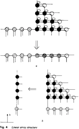
Observing Fig. 3, there are two permissable directions, k and j, for the second projection on the two-dimensional array, and the corresponding linear array structures are shown in Figs. 4a and b, respectively. Throughout the

c

approach, tag codes [11] are added to the DG to dis- tinguish the different functions on the index nodes. The tag code assignment is different from that of single projection in which only a line of index nodes are mapped into a PE. For double projections along the i and k or i and j directions, the index nodes of the k-i or j-i plane of the DG, respectively, will be mapped into a PE. Nodes with different functions in the same plane must therefore be assigned by different tag codes, so we assign 0 , 0 , 1,

2, 3', 3", 4 to the index nodes shown in Figs. 5a and b. Although the nodes marked with grey dots have the same function as others, their input data source is different from the others so we assign them with different codes ( 0 and 1). In Fig. 5a, we add four transfer nodes to the top of the plane to pop out the data. Note that the functions of nodes 0 and 0 , 3' and 3" (marked by 0 and 3, respectively) can be combined because no functional conflicts. Therefore, it needs five tag codes in these DGs in contrast to two tag codes in single projection cases. The final designs are shown in Figs. 6 and 7 which corre- spond to Figs. 4a and b, respectively. The FIFO length of each PE is four because the PES in Fig. 6 and Fig. 7 need four data computation. The data sequence of inputs, tag bits and the snap shot of operation at some operation instants is also shown in Fig. 6.

The operating functions of each PE and tag codes are also shown in the inset of Figs. 6 and 7. With more functions mapped into one PE, it is accordingly a little more complex than Fig. 3. The latencies in Figs. 6 and 7 are still the same as they need n(n

+

1)

+

n

+ n

= n2

+

3n - 1 and (n

+

1)(n

+

1) - 1 + n - 1 = n2

+

3 n - 1

clocks, respectively. This is because in each elimination

a

0 '

b

Fig. 4 Linear array structure

Y Second projection direction is along the k axis b Second projection direction is along the j axis

first and the second projections, a plane of index nodes on the DG are projected into one PE. Consequently, the index nodes with different functions will be mapped into a PE, and so the PE should have the capability to

perform different functions. To do this, the appropriate Fig, Tag code in DG control signals must be sent to the PE so that the correct

fUnCtiOn Of the PE will be performed in good time. In our

IEE PROCEEDINGS, Vol. 137, Pf. G, N o . 3, J U N E 1990

b

(1 Double projection directions are a,ong the, and axeS

b Double projection directions are along the i and j axes

(4)

step they need n

+

1 operations in each PE, and between each elimination step one time unit is needed to propagate data. Although the latency increases from (4n - 2) in Fig. 3 to (n2

+

3n

-

1) in Figs. 6 and 7, the array structure is reduced from two dimensions to one dimension. From the comparison between Figs. 6 and 7, it is clear that the design shown in Fig. 6 will therefore need

-

b2 a44 b l a14 a33 0 0 0 a22

b4 a14 b l a34 a43 0 0 a23 a32

b l a24 b3 a44 a13 0 a24 a33 a42

b2 a34 b4 a14 a23 b2 a34 a43 a12

a b b3 a44 _b4

C

(n

+

m) PES with n2 FIFO memory, (n

+

2m

+

1) input ports and one output port and 2n input lines for tags, whereas the design in Fig. 7 needs (n

+

1) PES with (n2

+

n) FIFO memory, four input ports and one output port and 2n input lines for tags, respectively. With hardware costs taken into consideration, the latter design is superior to the former, but it takes (n2

+

3) time units to

ul cll 00 0 0 0 0 O x O x O x a l l ulc21u2c12 0 0 0 0 0 x 0 x a12000 a21 ul ~ 3 1 ~ 2 ~ 2 2 ~ 3 ~ 1 3 0 0 0 x a13000a22001 a31 ulc41 u2c32u3c23u4c14 a14000 a23001 a32001 a41

U2 c42u3 c33 u4c24 a24001 a3001 a42001 u3CWU4C34 a34001 a43001 000

u4cL4 a44001 000 010

000 011 010 011 100 010 Fig. 6

along k direction of Fig. 3

a k = 4 b k = 3 c k = 2 d k = l

d Tag:

Linear arrays with local FIFO queues designedfrom projection

T d OOO c = a l d ; d = d ; n ' = c 001 o ' = a - e x d ; d ' = d ; e = c 010 d = n 011 c = a"id; d = d ; d I a 100 o ' = o " - c x d , d ' = d , c = c a d x x x x x x x x x x x x x x x x x x 010010010010011100100100011

-PE$-

x x x x x x x x x x x x01M)100100100111001001000110111M)1M)m011 x x x x x x 01001001M)10011100100100011011100100100011011100100100011 olooloolooloolll00lool00ollolll00~~ollolllooloolM)ollooooo1oo1oo1ooo

alla21a31a41a12a22a32a42 x a13 a23a33a43 xa14 a24a34a44x cll C21C31C41CI2 c22c32c42 xc13c23c33cwxc14 c24c34c44x U1 ul U1 ul U2 U2 U2 U2 x U3 U3 U3 U3 x U4 U4 U4 u4x b 1'00 bIOO bJOO

YE,

l l 0 ~ l l 0 I 110 j L! ! . J 810' a Fig. 7

along j direction of Fig. 3

b Tag: c Tag:

Linear arrays with local FIFO queues designedfrom projection

00 b = b + c x u OOO c = a i o " ; o ' = c 10 B = b = b " + c x u 001 a ' = a - a " x c ; c = c 11 No operation 010 d = d 011 c =din"; 6 =a''; a' = c 100 0' = d = a" x e, d = a", e = e 188 b 100 100 010 100 100 100 011 011 010 01 1 010 100 010 100 010 100 01 1 nin _ . 010 010 010 a' A

."h-'

i d C

(5)

input the data, whereas the design shown in Fig. 6 needs only (2n - 1). Observing the sequence of tag bits in Figs.

6 and 7, we see that if we change the tag bit value and the connection condition of the PE when the tag bit is pumped through the array, the function of codes 0 and 3,

1 and 4 are the same since their connections are suitably rearranged. This kind of modified design applied to Fig. 6 is shown in Fig. 8, where only two tag bits are required. The design shown in Fig. 7 can also be modified using a similar method. b2 a 4 4 b4 a14 b l a24 b2 a34 b l a14a33 b l a34 a43 b3 a44 a13 b4 a14 a23 0 0 0 a22 0 0 a23 a32 0 a24 a33 a42 b2 a34 a43 a12

@@ @

b3 a44 b4

0 0 0 a12 a21

0 0 a13 a22 a31

0 a14 a23 a32 a41

bl a24 a33 a42 b2 a34 a43

b3 a44 d '

b4

d Modijied design of Fig. 6 Fig. 8 a k = 4 b k = 3 e k = 2 d k = l Tag: 00 e = a i d ; d = d ; a' = a 10 a ' = a - c x d ; d = d ; c = c 01 a ' = e ; s e t d - - a " ; T a g = I I ; c = c I 1 a ' = c ; s e t a - - o " ; d ' = d ; c = c 3

In many real applications, matrix A in eqn. 1 is sparse especially when n is large, i.e. most entries of A are zeros. So if we fully utilise this property to modify the systolic array in Figs. 6, 7 and 9, to avoid trivial operations Linear systolic array with content addressable memory

R

a

Fig. 9A

along i and j axes, respectively

DG of solving eqn. I and array structures after projection

As to latency, the systems obtained by applying the second projection on Fig. 3 are not the best. Now, let us turn to the original 3-D DG which is redrawn in Fig. 9A. If the first projection is along the j direction instead of the i direction, then during each elimination step k it only needs (n

+

1 - k) operations in the PES as we can see in the DG, where only (n

+

1 - k) computations are projected into PES in the k direction. So, if the second projection is along the k direction, the latency is fn

+

1 - k)

+

2n - 1 = (n2

+

7n - 2)/2, where (2n - 1) is the time unit to propagate data between PES. Thus, a more efficient design is to choose the first projection to be along the j direction, and the resulting two- dimensional systolic-array system has the same latency 4n - 2 as in Fig. 3, but the PE number becomes n2. Then the second projection is along the k direction using the same procedures as in Figs. 6 and 7. The linear systolic array thus obtained is shown in Fig. 9B, which stores the elements of the same row in one PE. The latency of this design is (n2

+

7n - 2)/2 which is two times faster than that in Fig. 6, but the PE number is (2n - 1

+

m) with

(&'- n - 2) FIFO memory and four output ports which are larger than those of Fig. 6.

IEE PROCEEDINGS, Vol. 137, Pt. G , N o . 3, J U N E 1990

involving zero elements, and do not store the zero elements, then the computation of eqn. 1 may be speeded up and the storage amount be reduced.

But if we only store the nonzero elements of A, the data sequence that feeds the right PE at the right time will be destroyed. Thus, at each PE when the elimination step is carried out and the data are pipelining through PES to perform the elimination, we must search for the right data that have been stored in the local memory when doing the division or multiplication computations. This search requirement can be achieved by using the content addressable memories (CAM), in which part of the memory contents are used to search for the right data instead of using address. In this case, each PE stores the associated nonzero column (or row) elements in their local CAM.

The idea of using CAM for linear sparse matrix computation was first proposed in Reference 12. Figs. 10a

and b are the CAM systolic arrays designed from the modification of Figs. 6 and 9, respectively, with data format in arbitrary sparseness. The arrays for solving

B(t,) = B"(t,- ,)

+

C x U(t,) is not shown here for simpli- city. In this design, each data word must include four fields: the value of an element, its row (column) index, tag bits and an end-of-column (or end-of-row) indication bit. The tag bits have the same meaning as in Figs. 6 and 9. Because the data sequence is destroyed and the data cannot be piped into the array, they must be preloaded 189

(6)

into the CAM by a host computer. Also the tags can no longer be pipelined into the associated PE. So we attach

a44 x a33 x b l can sequentially pop out the data to the PE.

b4 a14 x a34 a43 x

k, the first job is to divide the row elements by the diagonal elements. Thus the CAM must have the ability of using the row (column) index to search for the data and

x b l a24 x b3 a44 a13

x x b2 a34 x b4 a14 a23

@@

a b

@

a22 0 0 0

a23 a32 0 0

a24 a33 a42 0

b2 a34 a43 a12

@@@

b3 a44 b4 C a l l 0 0 0 a12 a21 0 0

a13 a22 a31 0

a14 a23 a32 a41

bl a24 a33 a42

b2 a34 a43 b3 a44 b4

E h

a b

FOR (i from 1 ton){ Pop out elements of PE i ;

Transport the elements through the left(right) PES; According to the column(row) index to get data from CAM; Doing the multiplication or division according to the tag bits; }

C

a' Fig. 10 C A M systolic arrays Desimed from modification of

a a d tag PEA PE B 0 0 d = a d = a , r = T . s ' = s 1 0 c'=a/d a ' = (aS+a" . s) - c xd, c' =c, d - d , 0 1 d=a", T = T . s ' = s 1 1 Fig. 9B

tions along j and k axes

a k = 4 b k = 3 c k = 2 d k = l

r = T s ' = s

c' =a"/d,

r

= 10, s' = J

Linear arrays with local FIFO queues designed from projec-

the tag bits to the word to control the computation. The end-of-column (end-of-row) indication bit is used to signal the arriving of the last element of a column (row) so as to start the elimination steps started by the next column (row) elements. The row (column) index is used for CAM to search for the needed data in another column (row). The computation flow of Figs. 10a and b is

shown in Fig. 1Oc. Note that the diagonal elements of each column (row) are stored first in each PE so that, when popping out the data of column (row) k to carry out the kth elimination step, the correct data sequence can be obtained. This is because, in the elimination step 190

Y Fig. 6

b Fig. 9c by using the sparseness property of matrix A

The latency of the whole system is reduced from (n2

+

2n

+

1) and (nZ

+

7 n - 2)/2 to N A

+

n and

N Z

+

2n - 1 (excludes the time of loading input data)

for Figs. 10a and b, respectively, because the trivial com-

putations are avoided, where N A is the number of nonzero elements of matrix A and N Z is the number of nonzero elements along and below the diagonal. The memory requirement is also reduced from (tn' - n - 2) and n2 to N A

+

n and N A

+

N Z

+

2n - 1, respectively. Furthermore, the systolic array in Fig. 10a is superior to Fig. 10b not only because it has shorter latency and less hardware requirement, but also the data b( .) are needed after the nth time unit regardless of the sparseness of matrix A , whereas that in Fig. 10b is dependent on the sparseness of A . In real applications, especially when n is large, each row (column) of matrix A has only a few nonzero entries (3 to 4), so N A and N Z can be expressed

as r x n and (r x n

+

n)/2, respectively, where r denotes

the average number of nonzero elements in each row. Consequently, if we compare the computation time of the systolic array with FIFO, i.e. (n2

+

7 n - 2)/2, we find that much time is saved. In Wing [13], the LU decompo- sition method is used to solve A V = B and it took

N Z

+

5n - 2 time units to complete the computation,

whereas in our design of solving eqn. 1, which is much complex than solving A V = B, it takes only N A

+

n time units (which is less than N Z

+

5n - 2), since N A

+

n is less than N Z

+

5n - 2 as long as r

-=

9.

(7)

4

With the advance of VLSI technology, more PES can be integrated into one chip, but there are also physical limi- tations imposed by the number of 1/0 pins and yield. A natural solution is to divide the computation problem into smaller problems with a fixed size.

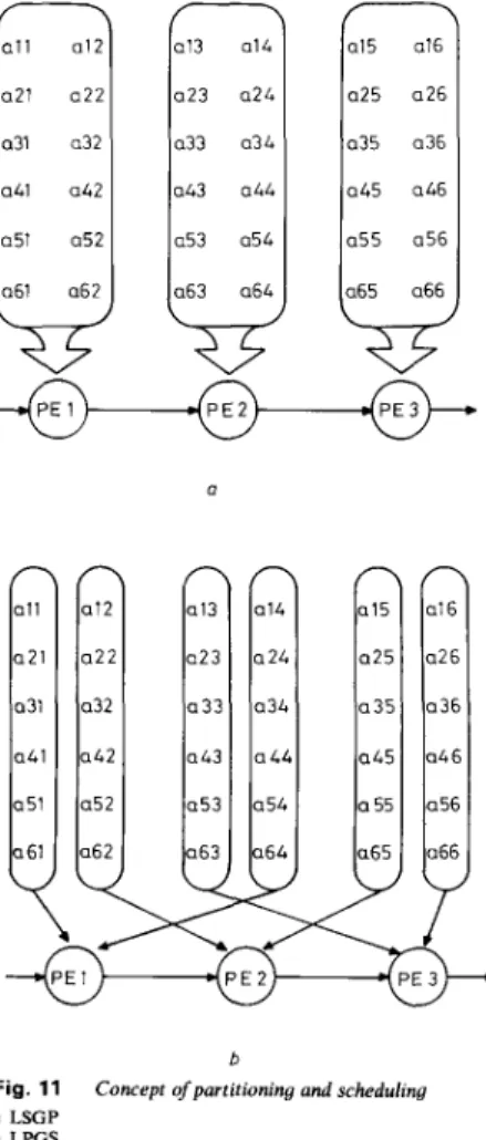
Many partition methods have been proposed to solve this problem [6, 14, 151. Roughly, according to the computation sequence of the data, they can be categorised into two types: i.e. local-serial-global-parallel (LSGP) and local-parallel-global-serial (LPGS) [6] which are illustrated in Figs. 1 la and b, respectively. Here, consider- ing the overlapping of two stages for solving eqn. 1, matrix A' is partitioned into r / p 1 submatrices of size

n x p by column. The partition scheme applied to the design of Fig. 10a is shown in Fig. 12A. As there are two independent iterated arcs on the DG so that the data will be changed iteratively along their propagation through the index nodes, global memories thereby become a necessity to save the intermediate results. The temporary results are popped out from the last PE into global memories and then fed into the first PE. Therefore, the data sequence can be maintained. By doing so, only global FIFO memories are required and one global feedback line and a switch box are needed in this partition scheme. The systolic array with local CAM and global FIFO is

Partition of linear systolic-array system

W

yw

b Fig. 11 a LSGP b LPGS

IEE PROCEEDINGS, Vol. 137, Pt. G , No. 3, J U N E I990 Concept of partitioning and scheduling

demonstrated in Fig. 12B, which is easily derived from Fig. loa. The data flow of the LPGS and LSGP partition schemes are shown in Figs. 12C and D, respectively. The

Fig. 12A Data partition ofmatrix A"

L

_{.. ..}

+

m

>

I

A ( n i p )

I

U 0 LL k

i

-

Fig. 1 2 8

C A M and global FIFO

Fixed size @) one-dimensional systolic array with local

FOR(/ from 1 to [nip]){ F O R ( j from i to [nip]){

IF(jequal i )

FOR(column k from 1 t o p of Ab,){

Sequently pop elements of the ( I - 1) x [nip1 + k column out from CAM of PE k top;

Normal Gauss-Jodan operation for matrix column from ( j - 1 ) x [nip1 + 1 to j x [n/p1;

} ELSE

FOR(each element in FIFO queue){ Sequently pop elements out from FIFO; Normal Gauss-Jordan operation for matrix column from ( j - 1) x ln/pl + k t o j x [nip]; }

Fig. 12C LPGS dataflows

FOR(/ from 1 ton){

Sequently pop elements of matrix column i from CAM of

P E ( ( / - l ) m o d p ) + l ;

Normal Gauss-Jordan operation for calumn from i to [n/p1 x p ; F O R ( j from [nip1 + 1 to (n/p1){

Sequently pop elements out from FIFO;

Normal Gauss-Jordan operation for matrix columns from ( j - 1 ) X p t o j X p ;

1

>

Fig. 1 2 D LSGP dataflow

size of the FIFO queue is determined by the nonzero elements of matrix A for the LPGS scheme or by the maximum number of nonzero elements in the column vector of matrix A for the LSGP scheme. The latency can 191

(8)

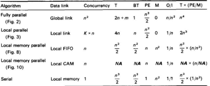
Table 1 : Analvses of various svlltolic a r r a v a s o l v i n g Ban. 1

___

Algorithm Data link Concurrency T BT PE M O/l T x (PE/M) Fully parallel

(Fig. 2 ) Global link n2

n3 2 n + m 1 - 0 nln’ n4 n2 Local link K x n 4n n - 0 l / n 2n3 Local parallel (Fig. 3) Local FIFO n

Local memory parallel (Fig. 8 )

Local CAM n Local memory parallel

(Fig. 10)

Serial Local memory 1

n2 n2

- n2 - n n2 1,h - x (n/n‘)

2 2 2

NA NA n NA l / n NA x (n/NA)

T=latency, BT=block pipelining period, PE=processor element, M=memory. K=variable from 1 t o n The number in this table is the order of the complexity

be computed as follows: LPGS :

WPl i - 1

latency =

1

(Nbi

+

p - 1) x (rn/pi - i) (rn/Pi(r/pi

+

1)) 2 = ((r

+

l)p - 1) x m 2 2P %_

-

LSGP: Inlpl latency = p

1

(r

+

p - 1) x ([/pi - i

+

1) i = l

where Nbi = rp is the number of nonzero elements in p column.

Due to the partition, the latency increases by a factor (n/2p), and a small array size will therefore pay a greater latency. The advance of using sparseness properties is to reduce the latency by a factor of (n/r).

5 Discussion

The one-dimensional linear systolic-array system with local FIFO, the linear systolic-array system with local CAM and the one-dimensional fixed-size linear systolic- array system with local CAM and global FIFO are all successfully designed by our D G approach. Which systolic array system is suitable to solve the problem is an interesting issue and would be determined by some prac- tical considerations. Table 1 summarises the comparisons of the features and performance for the various systolic- array systems. Besides those designs in this paper, the Table also includes a fully parallel design, which corre- sponds to a three-dimensional systolic-array system, and one processor system executing a serial algorithm, which may agree with the design obtained by triple projection on the three-dimensional DG.

6 A c k n o w l e d g m e n t

This work was supported by the National Science Council, Taiwan ROC under Grant NSC77-0201-EO09- 01.

7 R e f e r e n c e s

I KUNG, H.T., and LEISERSON, C.E.: ‘Systolic arrays for VLSI’. Proceedings of SIAM, Sparse Matrix Symposium, 1978, pp. 2 5 6 2 8 2 2 KUNG, S.Y., LO, S.C., and LEWIS, P.A.: ‘Optimal systolic design for the transitive closure and the shortest path problems’, IEEE Trans., 1987, C-36, (5), pp, 6 0 3 4 1 4

3 GACHET, P., JOINNAULT, B., and QUITTON, P.: ‘Synthesizing systolic arrays using DIASTOL’. International Workshop of Systol- ic Arrays, University of Oxford, Department for External Studies, 2 n d 4th July 1986, pp. F4.1LF4.12

4 CHEN, M.C.: ‘Synthesizing systolic design’. Proceedings of Interna- tional Symposium on VLSI Technology, Systems and Applications, Taiwan ROC, May 1985, pp. 209-215

5 MOLDOVAN, D.1.: ‘ADVIS: a software package for the design of systolic arrays’, IEEE Trans., 1987, CAD-6, (I), pp. 3 3 4 0 6 MOLDOVAN, D.I., and FORTES, J.A.B.: ‘Partition and mapping

algorithm into fixed size systolic arrays’, IEEE Trans., 1986, C-35, 7 FORTES, J.A.B., FU, K.S.,’ and WAH, B.W.: ‘Systematic approaches to the design of algorithmic specified systolic arrays‘. Proceedings of IEEE ICASSP, Piscataway, NJ, USA, 1985, pp. 891-895

8 L1, G.L., and WAH, B.W.: ‘The design of optimal systolic arrays’, IEEE Trans., 1985, C-34, (1). pp. 6 6 7 7

9 JOU, S.J., and JEN, C.W.: ‘The design of systolic array system for solving linear state equations’, IEE Proc. G , 1988, 135, (5), pp. 211-218

10 RAMAKRISHNAN, I.V., and VARMAN, P.J.: ‘Synthesis of an optimal family of matrix multiplication algorithms on linear array’, IEEE Trans., 1986, C-35, (11)

11 JEN, C.W., and HSU, H.Y.: ‘The design of a systolic array with tags input’. ISCAS, 1988, pp. 2263-2266

12 KIECKHAFER, R.M., and POTTLE, C.: ‘A processor array for factorization of unstructured sparse matrices’. IEEE International Conference on Circuits and Computers, 1982, pp. 38&382 13 WING, 0.: ‘A content-addressable systolic array for sparse matrix

computation’, J. Parallel Distrib. Cornput., 1985, pp. 17&181 14 NELIS, H., and DEPRETTERE, E.F.: ‘A systematic method for

mapping algorithms of arbitrarily large dimensions onto fixed size systolic arrays’. IEEE International Symposium on Circuits and System, 1987,2, pp. 559-563

15 NAVARRO, I.J., and LLABERIA, I.M., and VALERO, M.: ‘Parti- tion: An essential step in mapping algorithms into systolic array processors’, IEEE Cornput., 1987, pp. 77-88

16 LIU, C.-M., and JEN, C.-W.: ‘Design of algorithm-based fault- tolerant VLSI array processor’, IEE Proc. E, 1989, 136, (6), pp. 539-547

(I), PP. 1-12

192

.