A Three-Period Analysis of R&D Spillovers in the Presence of an Industry Life Cycle Pattern

全文

(1)International Journal of Business and Economics, 2009, Vol. 8, No. 1, 21-35. A Three-Period Analysis of R&D Spillovers in the Presence of an Industry Life Cycle Pattern Gamal Atallah* Department of Economics, University of Ottawa, Canada. Abstract This paper introduces the time dimension into the precompetitive R&D model, where both demand and spillovers vary over time. The effect of cooperation on R&D depends on a weighted function of spillovers, with the weights being a function of demand levels. The bulk of the incentives for innovation come from the growth phase of the industry. Key words: R&D cooperation; R&D spillovers; industry growth; product life cycle; technology diffusion JEL classification: L13; O33. 1. Introduction The goal of this paper is to analyze the impact of changes in R&D spillovers and demand during an industry life cycle on R&D incentives. There exists a large literature on technology diffusion, which has long recognized that information and technology take time to spread, and which have proposed different models to account for the evolution of diffusion over time (epidemic models, probit models, etc.). One of the most famous results in this respect is the diffusion S-shaped curve, whereby the diffusion rate first increases and then falls over time (see Geroski, 2000, for a comprehensive survey of the vast literature on diffusion). This gradual diffusion of technology has been overlooked by another literature, the non-tournament precompetitive R&D literature (key papers in this literature include Spence, 1984; d’Aspremont and Jacquemin, 1988; Kamien et al., 1992), which assumes that R&D spillovers are constant over time: once an innovation is made, spillovers occur instantaneously, overlooking the time path of diffusion. However, technologies do not diffuse instantly; rather, they diffuse gradually, with leakages increasing over time. The second dimension of industry growth which is taken into account is the Received September 19, 2008, revised March 10, 2009, accepted August 10, 2009. * Correspondence to: Department of Economics, University of Ottawa, Pavillon Desmarais, Room 10102, Ottawa, Ontario, K1N 6N5, Canada. E-mail: gatallah@uottawa.ca. The author would like to thank two editors of the IJBE and two anonymous referees for useful comments and suggestions which have significantly improved the paper..

(2) 22. International Journal of Business and Economics. change in demand: demand tends to grow initially, but as the industry matures and substitutes appear, demand declines (see Wang, 2004). Hence both spillovers and demand change during the life cycle of the industry. The interaction between changes in these two variables is the focus of this paper. The paper introduces time into the standard precompetitive R&D model and shows that the rate of change of spillovers and of demand, and not only their (average or final) levels, are crucial to understanding the incentives for R&D and the impact of cooperation on innovation. The paper sets up a model where firms invest in cost-reducing R&D and then compete in output. Output competition takes place over three periods, which correspond to the different growth and decline phases of an industry. Demand first increases and then declines over time, while spillovers always increase with time. It is shown that an increase in spillovers in one period tends to reinforce (mitigate) the negative effects of spillovers in other periods when both spillovers are sufficiently low (high). It is also shown that spillovers tend to have negative effects on R&D mostly during phases where demand is high: this is where the technology leakages hurt the innovating firm most. When demand is low, as during the introduction and decline phases, the effect of spillovers is much less important. Next, the incentives for innovation arising from different phases of the industry life cycle are analyzed. Much of the incentives for R&D come from the introductory period (because spillovers are low) and especially the growth period (because demand is high). The combination of low demand and high spillovers during the decline phase makes the contribution of this phase to R&D negligible. For plausible parameter values under R&D competition, the incentives provided by the introductory phase are higher than those provided by the decline phase, while the opposite is true under R&D cooperation. Finally, it is shown that the effect of cooperation on R&D depends on a weighted function of spillovers in all periods, where the weights are given by demand levels in each period. Hence, whether cooperation is beneficial for innovation depends not on a “unique” spillover level (which does not exist), but on the rate of change in spillovers over time, as well as the evolution of demand over time. The evidence in support of the gradual diffusion of technology is overwhelming. As Geroski (2000) notes: “Sometimes it seems to take an amazingly long period of time for new technologies to be adopted by those who seem most likely to benefit from their use” (p. 604). Mansfield (1985) reports a considerable time lag (an average of 18 months for 70% of firms in some industries) between the introduction of a technology and its leakage to competitors. Taking patent citations as a measure of diffusion, there is a considerable time lag between the time a patent is produced and the time it is cited by other patents (Caballero and Jaffe, 1993; Henderson et al., 1998), which is evidence of a diffusion lag. With respect to technology spillovers in particular, Geroski (2000) notes that: “few [economists] doubt that spillovers occur, although it is not clear how fast the process takes and what path the information flows take through the economy” (p. 607). Desmet and Rojas (2004) note that “spillovers take time to materialize” (p. 2), and show that in this context (in conjunction with absorption capacity constraints) gradual liberalization is the.

(3) Gamal Atallah. 23. appropriate policy, so as to give the country the time to benefit from foreign direct investment. Delays in the diffusion of spillovers and the adoption of technologies can be due to many factors: workers’ resistance (Canton et al., 1999), localization of knowledge spillovers (Jaffe et al., 1993; Keller, 2002; Adams, 2002), and the tacitness of knowledge. Baldwin and Lin (2002) report some of the difficulties associated with the adoption of advanced technologies, which may take time for firms to overcome (if at all): “education and training, time and cost to develop required software, and increased maintenance expenses” (p. 1). Interestingly, they find that users of advanced technologies report impediments to technology adoption at a consistently higher rate than non-users. They interpret this as an indication that users of new technologies are more aware of the problems they face, and spend the necessary resources to overcome those problems. Given the focus of the current paper, time is one such resource which may delay the adoption of new technologies. The issue of increasing diffusion rates has been addressed by Tse (2002) in an endogenous growth framework. He finds that a longer diffusion lag (which corresponds to a decrease in spillovers in the early periods in our model) improves the appropriability of R&D but also decreases its productivity; this is because in his model there is a diffusion lag within firms, which is related to the external diffusion lag. The present paper lies at the intersection of three different literatures: (1) the precompetitive R&D literature, which has emphasized investments in R&D, R&D cooperation, and appropriability; (2) the technological diffusion literature, which focuses on diffusion paths and adoption delays; and (3) the industry life cycle literature, which analyzes the evolution of demand over time. The model studied here incorporates the three key dimensions in these literatures: R&D investments (with and without cooperation), delayed R&D spillovers, and changing demand over time. As we will see, important interactions arise across these three dimensions. The organization of the paper is as follows. Section 2 presents and solves the model. Comparative statics are presented in Section 3, while Section 4 analyzes the effects of R&D cooperation. Section 5 looks at the relative contribution of the different phases of industry growth to the incentives for innovation. The last section concludes. 2. The Model There are two identical firms producing a homogeneous good and competing a la Cournot. At the outset, firms can invest in R&D to reduce their production costs, which may give rise to R&D spillovers benefitting the competitor. Both cooperative and noncooperative R&D are considered. There are three periods, denoted 1, 2, and 3, each corresponding to a different phase of the industry life cycle. The variables changing over time are demand and spillovers. It is assumed that demand first increases and then decreases as the product matures. Spillovers are always increasing from one period to the next..

(4) 24. International Journal of Business and Economics Period t is characterized by the level of demand At and the spillover rate. β t . It is assumed that A2 > A1 and A2 > A3 . Demand is at its highest during period 2, when the industry is growing rapidly; it is lower during the introductory phase (period 1) and the decline phase (period 3). Spillovers are such that β t ∈ [0,1] for all time periods, with 0 corresponding to no leakage and 1 corresponding to complete leakage of the technology. It is assumed that β1 ≤ β 2 ≤ β 3 : diffusion increases or remains unchanged over time but cannot decrease. Here β 3 − β 2 and β 2 − β1 represent the additional diffusion that takes place from one period to the next. This specification does not require that β1 + β 2 + β 3 ≤ 1 . It is the sum of the incremental spillovers in each period which is required not to exceed one. Hence, β1 + ( β 2 − β1 ) + ( β 3 − β 2 ) ≤ 1 , which requires only β 3 ≤ 1 . While typically spillovers and demand change in a continuous fashion, a discrete time model is much simpler to handle. Moreover, these three periods capture the main interactions between spillovers and demand. In period 1, the introductory phase, both demand and spillovers are low. In period 2, the growth and maturity phase, demand is high, while spillovers are intermediate. Finally, in period 3, demand is low, but spillovers are at their highest. The marginal production cost of firm i in period t is given by: ci ,t = α − xi − β t x j , i, j = 1, 2 , t = 1, 2, 3 .. (1). Here α represents the initial marginal production cost before accounting for any cost reduction due to innovation. The variable x represents R&D output, i.e., the marginal cost reduction in dollars. Firm i benefits fully from its innovation ( xi ) and benefits from the innovation output of its competitor ( x j ) through the period-specific spillover β t . It is assumed that At > α for all periods, otherwise the market would not exist in the absence of R&D. R&D is not time-specific: investments in R&D are made at the outset. Firm i benefits from its own R&D fully in each period. However, it benefits from the R&D of the other firm only gradually, as β t increases with time. This results in a marginal cost which is decreasing over time. This approach suggests a process through which production costs may decline over time even in the absence of subsequent innovation, simply due to increased diffusion over time. One could easily write a fully dynamic model, where R&D is performed in each period. The goal of the approach used here is to focus on the idea that for a given technology, the market conditions, represented by demand and spillovers, change over time, and that the diffusion of a given technology is gradual, irrespective of the fact that further discoveries are made while it is still being used. In contrast, demand and output are time-specific. Because spillovers (and hence production costs) and demand are time-specific, output will also vary over time. The inverse demand curve in period t is given by:. pt = At − y1,t − y2 ,t , t = 1, 2, 3 .. (2). Here pt represents the product price at period t , At the period-specific inverse.

(5) Gamal Atallah. 25. demand intercept, and yi , t the output of firm i in period t . For simplicity and without loss of generality, we disregard discounting. The profit of firm i over all periods is given by:. π i = ∑t =1 ( pt − ci ,t ) yi ,t −γ 3. xi2 , i = 1, 2 .. (3). Because the choices of output over the three periods are independent, it is equivalent to assume that output levels are chosen simultaneously or sequentially over time. To simplify, we assume a two-stage game. In the first stage, firms invest in cost-reducing R&D simultaneously. In the second stage, each firm chooses its output for all three periods simultaneously. The choice of output is independent of the presence or absence of R&D cooperation. Solving the output stage yields: yi ,t =. 1 ⎡ At − α + xi (2 − βt ) − x j (1 − 2β t ) ⎤⎦ , i, j = 1, 2 , t = 1, 2, 3 . 3⎣. (4). As we see, period t ’s output depends directly only on demand and spillovers in the same period. However, as we will see, because R&D depends on demand and spillovers in all periods, period t ’s output also indirectly depends on demand and spillovers in all periods. Substituting these output levels into the profit functions yields profits as a function of R&D expenditures. Maximizing the profits of each firm with respect to its R&D expenditures and using the symmetry of firms yields the noncooperative R&D output of each firm:. ∑. 3. xin =. t =1. (2 − β t )( At − α ). 9γ − ∑t =1 (1 + β t )(2 − β t ) 3. , i = 1, 2 .. (5). Under R&D cooperation, firms choose their R&D expenditures cooperatively to maximize their joints profits. Firms do not share information, hence the spillover rate is not affected by cooperation. The type of R&D cooperation studied here is R&D cartelization, following the terminology of Kamien et al. (1992). It would be straightforward to apply this model to research joint venture (RJV) cartelization, where firms also share information. The dynamic effects of spillovers would vanish under RJV cartelization, and only the effect of demand would remain. The cooperative R&D output of each firm is given by. ∑. 3. xic =. t =1. (1 + β t )( At − α ). 9γ − ∑t =1 (1 + β t ) 3. 2. , i = 1, 2 .. (6). While the solutions for R&D look similar to the summation of R&D output if firms faced three independent markets with three independent technologies (instead of three periods), the level of R&D is not equal to the independent market case because.

(6) International Journal of Business and Economics. 26. here the same level of R&D must respond to the incentives provided by different levels of demand and spillovers over time. Hence, total R&D cannot be written as an additively separable sum of the R&D that would obtain in each period. In the remainder of this paper we ask three questions. First, how do spillovers in one period affect the impact of spillovers in other periods? In other words, are there any intertemporal effects, meaning that the parameters of one period affect the sensitivity of R&D to the parameters of another period? Second, how does R&D cooperation affect R&D, and how does this effect depend on spillovers and demand? Third, how does each phase of the industry life cycle (introduction, growth, and decline) contribute to R&D investments? We are mainly interested in insights that go beyond the static one-period model. 3. Comparative Statics We first note that there are no surprises with respect to the effects of spillovers and demand on R&D. An increase in demand in any period increases (both cooperative and noncooperative) R&D. And an increase in spillovers reduces noncooperative R&D but increases cooperative R&D. These results are easy to verify from (5) and (6). Where the interdependencies between the periods occur is in the magnitudes of changes, i.e., how the level of spillovers in a given period affects the sensitivity of R&D to changes in spillovers in other periods. Proposition 1. Under R&D competition, an increase in spillovers in one period (say period i ) reinforces the negative effect of spillovers on R&D in another period (say period j ) if and only if:. {. 1 2(2 β i − 1)(2 β j − 1)ka + [(2β j − 1)( Ai − α ) + (2 β i − 1)( Aj − α )]kb kb3. }. (7). is negative, with k a and kb given by (9) and (10) below. An increase in spillovers in one period mitigates the negative effect of spillovers on R&D in another period if and only if (7) is positive. Proof. Consider first the interaction between β1 and β 2 . We find:. ∂ 2 xn 1 = {2(2 β1 − 1)(2 β 2 − 1)ka + [(2 β 2 − 1)( A1 − α ) + (2 β1 − 1)( A2 − α )]kb } ∂β1∂β 2 kb3. (8). where k a ≡ ∑t =1 ( At − α )(2 − β t ) 3. k b ≡ 9γ − ∑t =1 (1 + β t )(2 − β t ) . 3. (9) (10). Note that k a > 0 since At > α and β t ∈ [0, 1] for all periods by assumption..

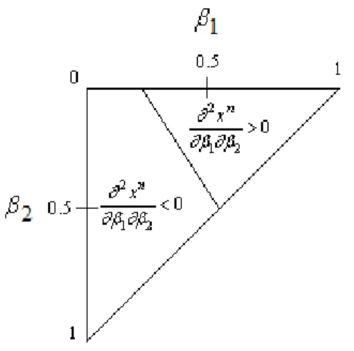
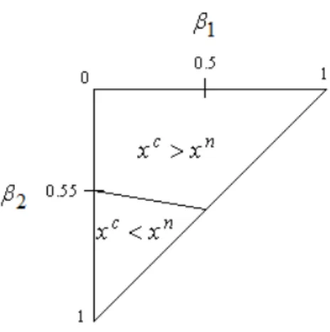
(7) Gamal Atallah. 27. Moreover, kb > 0 since k b is nothing but the denominator of xin and xin > 0 . This implies that the sign of the numerator of (7) is equal to the sign of the whole expression. The sign of the numerator depends on the magnitudes of β1 and β 2 . Evaluated at β1 = 0 and β 2 = 1 , the numerator yields: −2k a − ( A2 − A1 )k b < 0 .. (11). Evaluated at β1 = 1 and β 2 = 0 , the numerator yields: 2k a + [( A1 − α ) + ( A2 − α )]k b > 0 .. (12). Evaluated at β1 = β 2 = 0.5 , the numerator is zero. Hence this coordinate is on the locus of critical points where the cross effect is nil. To determine the shape of the locus of critical points, we solve for the value of β 2 which makes the numerator zero (this gives the combinations of β1 and β 2 such that the cross effect is nil) and differentiate with respect to β1 , which gives us the slope of the critical locus: −. ( A1 − α )( A2 − α )k b2 <0. [(4β 1 − 2)k a + ( A1 − α )k b ]2. (13). Putting these pieces of information together we can now plot the spillover space where the cross effect is positive and negative. Figure 1 illustrates this. Figure 1. Interaction between Spillovers in Periods 1 and 2. The same analysis applies to ∂ 2 x n ∂β 2 ∂β 3 , except that when evaluated at β 2 = 0 and β 3 = 1 , the sign of the derivative: −2k a + ( A2 − A3 )k b. (14).

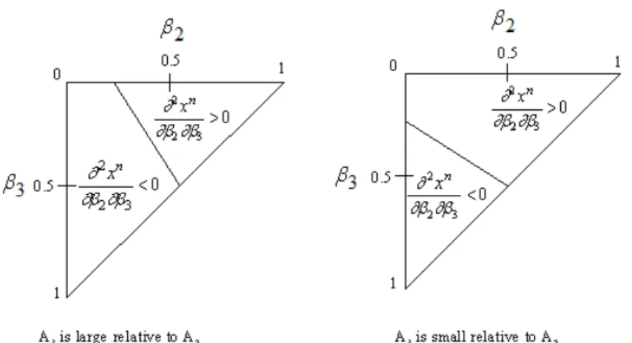
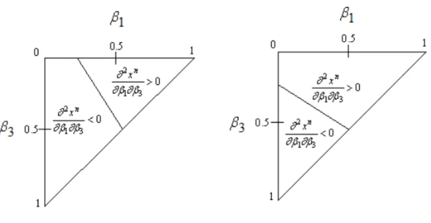
(8) 28. International Journal of Business and Economics. is ambiguous as the first term is negative and the second term is positive because A2 > A3 . Figure 2 illustrates the interaction between β 2 and β 3 . The left-hand side diagram obtains when A3 is large relative to A2 , while the right-hand side diagram obtains when A3 is small. Figure 2. Interaction between Spillovers in Periods 2 and 3. The same analysis applies also to ∂ 2 x n ∂β1∂β 3 , with the same exception mentioned above. In this case (11) becomes: −2k a + ( A1 − A3 )k b .. (15). The first term is negative, while the sign of the second term is ambiguous because we have not made any assumptions on whether output is greater during the introductory or the decline phase. But it remains true that the slope of the critical locus is negative. Figure 3 illustrates the interaction between β1 and β 3 . The left-hand side diagram obtains when A3 is large relative to A1 , while the right-hand side diagram obtains when A3 is small. By the symmetry of cross derivatives, ∂ 2 x n ∂β i ∂β j = ∂ 2 x n ∂β j ∂β i . Hence, to say that β i mitigates the negative effect of β j implies also that β j mitigates the negative effect of β i . It follows from Proposition 1 that spillovers from different periods tend to reinforce each other’s negative effects when both spillovers are sufficiently low, while they tend to mitigate each other’s negative effects when both spillovers are sufficiently high. The intuition behind this result is that with low spillovers, an increase in spillovers hurts the firm more than they benefit it, hence the firm tends to reduce R&D. On the other hand, with high spillovers, an increase in spillovers benefits the firm more than it hurts it; hence the negative effect of spillovers on R&D is mitigated. In the analysis of the interactions between β1 and β 3 on one.

(9) Gamal Atallah. 29. hand and between β 2 and β 3 on the other hand, there was some ambiguity as to the location of the left end of the locus of critical points. It can be either at some point where β 3 = 1 (the left-hand side diagrams in Figures 2 and 3), or it can be at some point where β1 = 0 or β 2 = 0 (the right-hand side diagrams in Figures 2 and 3). According to (14) and (15), the left-hand side diagram is more likely to obtain, i.e., the effect is more likely to be negative, when output in the high spillover period ( A3 ) is not too low relative to A1 and A2 . A relatively high level of output in the high spillover period increases the negative effects of spillovers, increasing the likelihood that spillovers reinforce each other’s negative effects. Figure 3. Interaction between Spillovers in Periods 1 and 3. Because β 3 ≥ β1 , the relationship between β 2 and β 3 is more likely to be one of mutual mitigation of negative effects than the relationship between β1 and β 2 . For instance, an increase in β1 is more likely to mitigate the negative effect of β 3 than to do the same thing for β 2 . An increase in β 2 is more likely to reinforce the negative effect of β1 and to mitigate the negative effect of β 3 . Finally, an increase in β 3 is more likely to mitigate the negative effect of β 2 than to do the same thing for β1 . It would seem that an increase in β 3 is the most beneficial: its direct effect is negligible, because output is low during that period. Furthermore, its indirect effects are the most likely to be beneficial. We do not study the equivalent comparative statics under R&D cooperation because in that case spillovers have non-ambiguous positive effects on R&D, and their positive effects simply tend to reinforce each other between the different periods. Rather, in the next section we tackle directly the effect of cooperation on R&D..

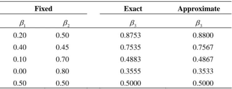
(10) 30. International Journal of Business and Economics. 4. The Effect of R&D Cooperation. It is well known that in the absence of information sharing, R&D coordination tends to increase R&D investments when spillovers are sufficiently high (see d’Aspremont and Jacquemin, 1988). What we obtain here is a generalization of this result. Proposition 2. R&D cooperation increases R&D output if and only if:. ∑. 3 t =1. ( At − α )(2 β t − 1) > 0 .. (16). Proof. We take the difference xic − xin :. ∑ =. 3. x −x c i. n i. t =1. (1 + β t )( At − α ). 9γ − ∑t =1 (1 + β t ) 3. 2. ∑. 3. −. t =1. (2 − β t )( At − α ). 9γ − ∑t =1 (1 + β t )(2 − β t ) 3. .. (17). Instead of using this exact difference, which gives a cumbersome expression, we note that the denominators of these two expressions are very close, and hence the sign of the difference is determined mainly by the numerators. Taking the difference between the numerators yields (16). To verify that this is an acceptable approximation of the effect of cooperation, Table 1 fixes β1 and β 2 and derives the critical value of β 3 such that cooperation does not change total R&D using two methods: the approximation given by (16), and the exact difference given by (17). It is clear that the critical values of β 3 using the two methods are essentially identical. Table 1. Critical Values of Spillovers Determining the Effect of Cooperation: Exact and Approximate Calculations Fixed. Exact. Approximate. β3. β3. β1. β2. 0.20. 0.50. 0.8753. 0.8800. 0.40. 0.45. 0.7535. 0.7567. 0.10. 0.70. 0.4883. 0.4867. 0.00. 0.80. 0.3555. 0.3533. 0.50. 0.50. 0.5000. 0.5000. If (16) is positive, then R&D cooperation increases innovation, and if it is negative then R&D cooperation reduces innovation. It is still true here that higher levels of spillovers in any period increase the likelihood that cooperation will increase R&D. Whether the contribution of each period is positive or negative depends on whether β t is greater than or less than 0.5. This is reminiscent of the standard result in the literature. Here, however, the spillover rate of each period is.

(11) Gamal Atallah. 31. weighted by the output of that period. Because the growth period (period 2) has the highest output, its spillover carries the most weight in determining the effect of cooperation. Therefore the effect of R&D cooperation depends on a weighted function of spillovers, with the weights given by the market size ( At − α ) in each period. To illustrate the effect of cooperation, we fix the parameters of the model as follows: A1 = 1000 , A2 = 2000 , A3 = 1000 , β 3 = 0.9 , α = 50 , γ = 60 . Figure 4 illustrates the regions where cooperation increases (decreases) R&D in ( β1 , β 2 ) space. The figure illustrates that when β1 and β 2 are sufficiently low, R&D cooperation decreases R&D, while it increases it if they are sufficiently high. β 2 is much more important in determining the effect of cooperation (the separating line is almost horizontal). This is because of the higher weight provided by A2 . Figure 4. Effect of Cooperation on R&D. 5. The Incentives for Cooperation. The total investment in R&D depends on the sum of the incentives provided by profits in each period. The allocation of these incentives between the different periods in our model depends on demand and spillovers. It is possible to decompose total R&D investment into the incentives provided by each period. From (5) we define the share of incentives for noncooperative R&D attributable to period t as: S tn =. (2 − β t )( At − α ) . 3 9γ − ∑t =1 (1 + β t )(2 − β t ). (18). This share represents the share of total R&D that can be attributed to period t , given the level of spillovers and demand in all periods. As expected, this share increases with At and decreases with β t . Similarly, from (6) we define the share of incentives for cooperative R&D attributable to period t as:.

(12) 32. International Journal of Business and Economics S tc =. (1 + β t )( At − α ) 9γ − ∑t =1 (1 + β t ) 3. 2. .. (19). In the cooperative case, the share increases with both demand and spillovers. It is useful to analyze how the incentives for R&D vary per period and depend on the type of interaction in R&D. Proposition 3. In this context the following conclusions can be drawn.. (a) Stn > Stc if and only if β t < βt' =. β j + β j2 + β l + βl2 − 3γ , j, l ≠ t . 2 + β j + β l − 6γ. (20). (b) S 2n > S3n . (c) S 2c > S1c . Proof. We consider each statement in turn. First, we can write: ⎡ ⎤ 2 − βt (1 − 2β t ) ⎥ (a) Stn − Stc = ( At − α ) ⎢ − 2 3 ⎢ 9γ − 3 (1 + β )(2 − β ) ⎥ 9γ − ∑ t =1 (1 + β t ) ⎦⎥ ∑ t =1 t t ⎣⎢. (21). Setting this difference equal to zero and solving for the critical value of β t yields the solution. Next, observe that: (b) S 2n − S3n =. ( A2 − α )(2 − β 2 ) − ( A3 − α )(2 − β 3 ) 9γ − ∑ t =1 (1 + β t )(2 − β t ) 3. .. (22). This difference is positive because A2 > A3 and β 3 > β 2 . Finally, notice that: (c) S 2c − S1c =. ( A2 − α )(1 + β 2 ) − ( A1 − α )(1 + β1 ) 9γ − ∑ t =1 (1 + β t ) 3. 2. .. (23). This difference is positive because A2 > A1 and β 2 > β1 . Proposition 3(a) states that, in comparing the incentives for innovation in a given period between cooperation and no cooperation, the incentives under no cooperation will be higher provided β t < β t′ , where the critical threshold β t′ depends on spillovers in other periods and on the cost of R&D. Interestingly, higher spillovers in other periods reduce β t′ , making it more likely that the incentives are higher under cooperation; in this sense, spillovers in other periods act as substitutes for spillovers in the current period. Again, this illustrates the interactions between periods. Proposition 3(b) establishes that, under no cooperation, the incentives from period 2 are always higher than those from period 3 because A2 > A3 and β 3 > β 2 . Proposition 3(c) shows that, under cooperation, the incentives from period 2.

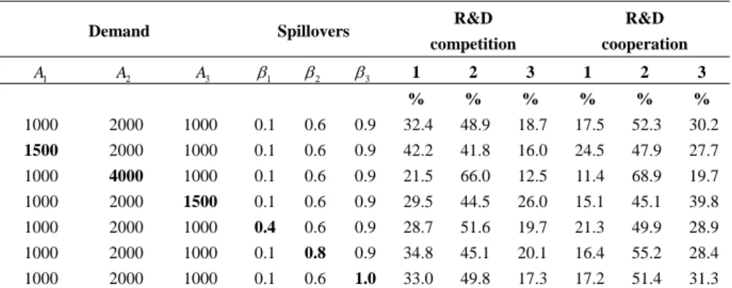
(13) Gamal Atallah. 33. dominate those from period 1 because A2 > A1 and β 2 > β1 . Other comparisons between the shares of total incentives attributable to each period depend on the levels of demand and spillovers and cannot be ranked unambiguously. To give an idea about the magnitudes of the relative shares, Table 2 illustrates the relative shares for different parameter values. The first row represents the benchmark case, and subsequent rows represent variations in one parameter relative to this benchmark. We can see that the bulk of the incentives for R&D comes from the growth phase of the industry. Moreover, because spillovers have a negative effect under R&D competition, period 1 provides more incentives than period 3 in this case. At the same time, spillovers have a positive effect on R&D under R&D cooperation. Hence, period 3 provides more incentives than period 1 under R&D cooperation. The results in this table are sensitive to demand and spillover levels, however. Table 2. The Relative Contribution of the Different Phases to Innovation Demand. A1. A2. Spillovers. A3. β1. β2. β3. R&D. R&D. competition. cooperation. 1. 2. 3. 1. 2. 3. %. %. %. %. %. %. 1000. 2000. 1000. 0.1. 0.6. 0.9. 32.4. 48.9. 18.7. 17.5. 52.3. 30.2. 1500. 2000. 1000. 0.1. 0.6. 0.9. 42.2. 41.8. 16.0. 24.5. 47.9. 27.7. 1000. 4000. 1000. 0.1. 0.6. 0.9. 21.5. 66.0. 12.5. 11.4. 68.9. 19.7. 1000. 2000. 1500. 0.1. 0.6. 0.9. 29.5. 44.5. 26.0. 15.1. 45.1. 39.8. 1000. 2000. 1000. 0.4. 0.6. 0.9. 28.7. 51.6. 19.7. 21.3. 49.9. 28.9. 1000. 2000. 1000. 0.1. 0.8. 0.9. 34.8. 45.1. 20.1. 16.4. 55.2. 28.4. 1000 2000 1000 0.1 0.6 1.0 33.0 49.8 17.3 17.2 51.4 31.3 Notes: A bold number indicates that this variable has changed relative to the benchmark case (row 1).. In addition to indicating how the incentives for innovation are distributed over time, these shares are useful to give an idea of how firms’ investments in R&D would evolve over time. If firms could make a new investment at the beginning of each period, most of the incentives for R&D at each period would be determined by the level of spillovers and demand at that period; hence these shares are an indication of what firms’ investments would be in a model with repeated investments in R&D. Such a model could easily be derived based on the framework provided here. From a policy point of view, these results suggest that extending protection in time, especially over the last phases of the life cycle of the product, is not very effective because at that stage demand is relatively low. A more effective approach would be to strengthen protection when demand is still high. And this is true whether the regime is one of R&D competition or R&D cooperation. Under R&D competition, extending protection would not be very effective because of low output in period 3. Whereas under R&D cooperation, extending protection would actually provide negative incentives, since spillovers increase R&D under R&D cooperation..

(14) 34. International Journal of Business and Economics. 6. Conclusions. The goal of this paper was to analyze the effect of the evolution of demand and spillovers on the incentives for innovation. The paper presented three main results. The first pertains to the intertemporal linkages involving spillovers. It was shown that an increase in spillovers in one period tends to reinforce (mitigate) the negative effects of spillovers in other periods when both spillovers are sufficiently low (high). Second, the effect of cooperation on R&D depends on a weighted function of spillovers, with the weights being a function of demand levels. Finally, the bulk of the incentives for innovation come from the growth phase of the industry. With R&D competition, the incentives provided by the introductory phase are higher than those provided by the decline phase, while the opposite is true under R&D cooperation. Overall, the paper shows that what matters for the incentives for innovation is not only the level of spillovers, but also their rate of change, as well as their interaction with demand changes over the product life cycle. From the demand side, if new products have shorter life cycles, then spillovers become less important, because by the time they have become high it is likely that the product is well into its decline phase and is being replaced by more modern substitutes. This causes high spillovers to become less of a disincentive because the output affected by these high spillovers is lower. In fact, a shorter product life cycle may have a mixed effect on the incentives for R&D: negative incentives because total sales are lower; but positive incentives because a larger portion of these sales are made more quickly, hence while spillovers are lower. From the supply (technology) side, if new production processes are replaced more often by more modern ones, then competitors have less time to benefit from copying those processes; hence spillovers become less important because by the time the technology is well known it is already being replaced by a more modern production process. The evolutions of spillovers and demand also have implications for the protectionist measures taken by firms. Firms may have more incentives to invest in protective measures aiming at reducing spillovers during the initial phase (in anticipation of the coming growth phase) and during the growth phase (because of high output). They are less likely to do so during the decline phase of the product or technology. Time is an important dimension which was overlooked by most of the non-tournament R&D literature, especially with respect to the fact that technologies diffuse gradually throughout the economy. While for some purposes the static model, where demand and spillovers can be seen as a weighted average of demand and spillovers over the industry life cycle, may be acceptable, other types of analysis may require accounting explicitly for changes in demand and spillovers over time..

(15) Gamal Atallah. 35. References. Adams, J. D., (2002), “Comparative Localization of Academic and Industrial Spillovers,” Journal of Economic Geography, 2(3), 253-278. Baldwin, J. and Z. Lin, (2002), “Impediments to Advanced Technology Adoption for Canadian Manufacturers,” Research Policy, 31, 1-18. Caballero, R. J. and A. B. Jaffe, (1993), “How High Are the Giants’ Shoulders: An Empirical Assessment of Knowledge Spillovers and Creative Destruction in a Model of Economic Growth,” in NBER Macroeconomics Annual, O. Blanchard, and S. Fischer eds., Cambridge, MA: MIT Press. Canton, E. J. F., H. L. F. De Groot, and R. Nahuis, (1999), “Vested Interest and Resistance to Technology Adoption,” Center for Economic Research, Tilburg University Discussion Paper, No. 106. d’Aspremont, C. and A. Jacquemin, (1988), “Cooperative and Noncooperative R&D in Duopoly with Spillovers,” American Economic Review, 78(5), 1133-1137. Desmet, K. and J. A. Rojas, (2004), “Foreign Direct Investment and Spillovers: Gradualism May Be Better,” Departamento de Economía, Universidad Carlos III de Madrid Working Papers, No. 04-04. Geroski, P. A., (2000), “Models of Technology Diffusion,” Research Policy, 29, 603-625. Henderson, R., A. B. Jaffe, and M. Trajtenberg, (1998), “Universities as a Source of Commercial Technology: A Detailed Analysis of University Patenting, 1965-1988,” Review of Economics and Statistics, 80(1), 119-127. Jaffe, A. B., M. Trajtenberg, and R. Henderson, (1993), “Geographic Localization of Knowledge Spillovers as Evidenced by Patent Citations,” Quarterly Journal of Economics, 108(3), 577-598. Kamien, M. I., E. Muller, and I. Zang, (1992), “Research Joint Ventures and R&D Cartels,” American Economic Review, 82(5), 1293-1306. Keller, W., (2002), “Geographic Localization of International Technology Diffusion,” American Economic Review, 92(1), 120-142. Mansfield, E., (1985), “How Rapidly Does New Industrial Technology Leak Out?” Journal of Industrial Economics, 34(2), 217-223. Spence, M., (1984), “Cost Reduction, Competition, and Industry Performance,” Econometrica, 52(1), 101-121. Tse, C. Y., (2002), “The Diffusion of Knowledge and the Productivity and Appropriability of R&D Investment,” Journal of Economic Dynamics and Control, 26(2), 303-331. Wang, Z., (2004), “Learning, Diffusion, and the Industry Life Cycle,” Federal Reserve Bank of Kansas City Working Paper, No. 04-01..

(16)