Nonlinear Adaptive Speed and Torque Control
of Induction Motors with Unknown
Rotor Resistance
An-Ming Lee, Li-Chen Fu, Member, IEEE, Chin-Yu Tsai, and Yu-Chao Lin
Abstract—In this paper, we propose a nonlinear adaptive speed
and torque controller of induction motors with unknown rotor re-sistance. All the system parameters except rotor resistance are as-sumed to be known, and only the stator currents and rotor speed are assumed to be available. The desired speed and torque should be a smooth bounded function. A complete proof of the global sta-bility without singularity is given, and the output error will con-verge to zero asymptotically. Finally, the simulation and experi-mental results will be given to demonstrate the effectiveness of the proposed controller.
Index Terms—Adaptive tracking control, induction motors,
par-tial-state feedback, unknown rotor resistance.
NOMENCLATURE -axis ( -axis) stator voltage. -axis ( -axis) stator current. -axis ( -axis) rotor flux.
Mechanical angular speed of rotor. Stator resistance.
Equivalent rotor resistance. Stator self-inductance.
Equivalent rotor self-inductance. Mutual inductance.
Number of pole pairs. Rotor inertia. Damping coefficient. Load torque. Torque constant [ ]. [ ]. . . . I. INTRODUCTION
D
UE TO THE highly nonlinear dynamics, the control of an induction motor has become the benchmark of nonlinear control theory and has been extensively explored over the past decade. In the early years, much of the research was devotedManuscript received July 23, 1997; revised December 18, 1998. Abstract pub-lished on the Internet December 18, 2000.
A.-M. Lee, C.-Y. Tsai, and Y-C. Lin are with the Department of Electrical Engineering, National Taiwan University, Taipei 106, Taiwan, R.O.C.
L.-C. Fu is with the Department of Electrical Engineering and Department of Computer Science and Information Engineering, National Taiwan University, Taipei 106, Taiwan, R.O.C.
Publisher Item Identifier S 0278-0046(01)02638-7.
to the control problems with full-state feedback, and either ob-tained the approximate stator–rotor flux decoupling or achieved exact input–output linearlization. So far, there have been sev-eral methods developed, such as the nonlinear geometric tech-niques [5], [8], or their adaptive version [9]. Although these control schemes could achieve satisfactory performance with mildly complex calculations, they have exhibited the problem with singularity and, in practice, the full-state feedback is unde-sirable since the rotor fluxes are very difficult to measure accu-rately.
In recent years, due to the great advances in nonlinear con-trol theory, the observer-based concon-troller has become one of the most commonly used schemes in induction motor control and an enormous amount of results on this have been published. In-stead of measuring the rotor fluxes directly, the flux observers were constructed to furnish flux estimates needed in the con-troller. First of all, Kanellakopoulos et al. [4] proposed a non-linear flux-observer-based speed control with known motor pa-rameters. Thereafter, a variety of related research has also been presented [1], [10], [14].
All the control schemes mentioned above, whether full-state or partial-state feedback, are greatly dependent on the exact knowledge of the motor parameters. However, these are very sensitive to the variation of temperature and the environment of operation. Therefore, to attain the high control performance with sufficient robustness, the contemporary design of the in-duction motor controller should take the uncertainties of motor parameters into account. In [11], Marino et al. proposed a clever adaptive observer scheme which could compensate for the un-known but bounded rotor resistance. Later, Hu et al. [3] slightly modified the above observer structure and provided a rigorous proof for speed/position control with an uncertain mechanical subsystem. However, it was still subject to a singularity problem when the magnitude of the estimated rotor flux is zero.
For the torque control problem, many results have been pre-sented and they have obtained satisfactory performance. In [2], Espinosa et al. proposed a globally stable output-feedback speed tracking controller for induction motors without any estimation of the rotor fluxes. However, this scheme needs to know exact values of the motor parameters.
In this paper, we will propose a new nonlinear adaptive speed and torque controller with unknown rotor resistance, which is free of the singularity problem. Only the stator currents and rotor speed are assumed available for the design. A complete Lya-punov-based proof is provided which shows that the errors of speed and torque tracking will asymptotically approach to zero. 0278–0046/01$10.00 © 2001 IEEE
The simulation as well as the experimental results are also pre-sented to demonstrate the performance and effectiveness of the hereby developed controller.
The organization of this paper is as follows. Section I briefly gives an introduction about induction motors and surveys some related research. In Section II, the mathematical model of an in-duction motor will be presented in detail. The state observers and controller design are developed in Section III, in which the asymptotical speed and torque tracking will be proved, and the simulation results of the control performance are given in Sec-tion IV. Finally, we will make some conclusions in SecSec-tion V.
II. PRELIMINARY ANDPROBLEMFORMULATION
A. Mathematical Modeling
If the induction motor is assumed to be linear, i.e., it is never in the saturation region, and the waveform of air-gap magne-tomotive force (MMF) is nearly sinusoidal, then the dynamic equations of the induction motor can be expressed as follows [6], [3]:
(1)
where and are constants defined in the
Nomen-clature. In the above equations, are referred to
as the well-known stator fixed – model as presented in [3]. Moreover, to facilitate our subsequent controller design which intends to relax the need of the knowledge of the rotor resistance , the terms associated with are separated from the other terms in the system dynamic equations.
B. Problem Statement
Given the above equations, the control objective is now to design a nonlinear adaptive speed and torque servo controller of the induction motor with unknown rotor resistance which guar-antees the asymptotical stability of the closed-loop system. In this paper, we will focus on the speed and torque tracking con-trol, or, servo control with satisfactory performance, i.e., given the desired speed and torque trajectories, the controller should be able to control the induction motor to track those trajecto-ries as closely as possible. Moreover, we only need to know the upper and lower bounds of the rotor resistance instead of its exact knowledge.
III. INDUCTIONMOTORSCONTROL
A. Problem Description
Before we proceed with the controller design and its analysis, some practical assumptions will be made as follows.
Assumptions:
A1) All the parameters of the motor except the rotor
resis-tance are known.
A2) The stator currents and rotor speed are measurable sig-nals.
A3) The rotor resistance is unknown but its upper and lower bounds are priorly known, i.e.,
for some known constants and .
A4) The desired torque should be bounded continuously
differentiable, i.e., .
A5) The load torque is a function which satisfies that, if is bounded, then the rotor speed is also bounded.
Remark 1: In general, the load torque is a function of the
rotor speed. In this paper, we will assume that the load torque can be expressed in the following form:
for some constants , and the sigmoidal
func-tion . This form
in-cludes the viscous friction, coulomb friction, and mechanical
load. From the torque–load relation ,
where is the rotor inertia, and is the damping coefficient. Due to the fact that the flux signals are not measurable (be-cause lack of practical flux sensors), the nonlinear adaptive con-troller proposed here will have to involve state observation and, hence, the observer design.
B. State Observer Design
From the dynamic equations in (1), it is clear that many terms on the right-hand side (RHS) of the expressions involving
and those involving are the same.
Therefore, motivated by the observer scheme in [3], in addition to the flux observers, we construct the current observers which takes the unknown rotor resistance into account. Define the observation errors as follows:
and the following auxiliary weighted observation quantities: (2) Let the state observers be designed as follows:
(3) where is a design parameter which is quite important
for subsequent stability analysis, and , , , are
Combining (1) and (3), we can obtain the following sets of dynamic equations of observation errors:
(4) whereby and can be straightforwardly derived as
(5) which clearly are computable since are both
avail-able signals and , , and are all design signals.
Comparing (4) and (5), it can be easily seen that the RHS of (5) does not depend on any unknown parameters or signals, unlike the situation for (4). This motivates us to build an observer for , , which leads to additional observation errors , de-fined as follows:
where indicate the errors caused by the initial conditions, i.e.,
Because are not priorly known, and can be
regarded as some unknown constants.
Using the related terms presented above, we now design the observer inputs to achieve the necessary stability prop-erty as follows:
(6)
Remark 2: Note that the terms introduced in the design of
and are to cancel the unmeasurable terms in the observer error dynamics so that a well-known Lyapunov stability analysis can be made.
Likewise, the input signals and are designed as fol-lows:
(7)
Given the input design of , for the observer,
we can simplify the dynamic equations (5) as
Now, construct a Lyapunov function candidate as follows:
and substitute , and into its time derivative ,
then, we can obtain the following result:
where
and (in fact, ) are some auxiliary
inputs yet to be specified.
C. Nonlinear Adaptive Controller Design
Define the state variables in a more compact form as follows:
then, the state equations can be written concisely in a matrix form as follows:
where , and are defined at the bottom of the next page.
Remark 3: From the foregoing compact redefinition, we can
observe that, is a negative-definite matrix, so that .
1) Torque Control:
Lemma 1: If the desired torque can be expressed in the following form:
then the bound on the difference between the electrical torque and the desired torque can be expressed as follows:
where
Proof: Please refer to [14].
With this lemma, it is quite obvious that the following corol-lary will naturally hold.
Corollary 1: If the state error as , then
as .
As a result, we can realize that the objective of torque tracking will be achieved once the state tracking is achieved. This, thus, allows us to concentrate on the dynamics of state tracking error as derived in the following:
(9) where
with
In the above equations, the input voltages and can be used to completely eliminate the terms of and . However, there are not enough inputs which can be used to cancel and . Therefore, we will regard the desired currents and fluxes as the pseudo inputs and design them properly so as to make the error system asymptotically stable.
Now, choosing the desired fluxes and currents as follows:
(10) for some constant , we can directly get the following result:
It can, in fact, be verified that the choice (10) will satisfy the
condition in Lemma 1, namely, .
Besides, the desired fluxes and currents are also subject to the following condition.
Corollary 2: If is a bounded function, then
( ), namely, the desired fluxes and
cur-rents, are all bounded functions.
Proof: Please refer to [14].
Now, we are ready to introduce our control law as well as to analyze the resulting system stability. Select the Lyapunov function candidate as follows:
diag
for some constants , then its first-order time deriva-tive can be found as follows:
(11)
where . From the definitions of and ,
it is clear that and are both measurable since they can be expressed as follows:
Let the control inputs and be designed as follows:
(12) for some constant , where and are another auxiliary control inputs to be defined later, then it is clear that such control is indeed realizable.
Therefore, by substituting and into (11) and using the
inequality of , we can attempt to derive
the upper bound on as follows:
(13)
where one has to beware that the terms of and are not measurable. Following a similar way of designing and , we let the auxiliary control inputs and be designed mainly to cancel those terms with either positive or uncertain sign.
Suppose and are designed as follows:
(14) which again is a realizable design. After somewhat ingenious manipulation, we have
which along with the relation , derived from the
proof of Lemma 2, can allow us to rederive the upper bound on as
where
So far, we have presented the design of control inputs, and , as well as the previous observer design, namely, . In order to complete the whole adaptive control design and to analyze the overall system stability, we choose a natural Lyapunov function candidate as follows:
To evaluate its time derivative, obviously we only need to sum up the time derivatives of and as follows:
which with the following design of auxiliary inputs:
(15) apparently leads to a much more concise form for the estimate of
(16)
Fig. 1. Control block diagram.
where , and for some constants . By
Lyapunov stability theory, all the signals involved in the system will be bounded provided the RHS of (16) can be established to be nonpositive. Clearly, it is not the case now simply because of the last term on the RHS of (16).
Remark 4: In general, the value of is several and is hundreds of millihenrys and, therefore, we can directly make an assumption that
Since is not measurable so that the last term on the RHS of (16) cannot be easily canceled, we can design a projection law to eliminate it as follows to serve this purpose:
if if where the initial condition of should satisfy
for some constants , so that (16) can be further sim-plified as
(17)
By assigning properly, and , it can be
shown that and are all
bounded. From Corollary 2, are bounded
and, hence, are also bounded. By definitions of
, it is obvious that and are also bounded. Since the true states and the estimated errors are all bounded, then the state estimations are also bounded. Therefore, all the internal signals and, hence, the signal as well as are bounded and, especially by assumption A5), from (9) and
from (9) are all bounded as well.
As a consequence, all the input design is, indeed, a feasible design and by Barbalat’s Lemma, it can be shown that
as (18)
and, according to the results of Lemma 1,
(19) This shows that the objective of torque tracking is, thus, achieved. The following is a summarization of this result.
Fig. 2. ! = 1000(1 0 exp ) r/min.
Theorem 1: Consider an induction motor whose dynamics
are governed by (1) under the assumptions A1)–A5). Then, the output electrical torque will approach the desired torque asymptotically by the following controller:
for some constant , where subject to (4)
and the auxiliary control inputs , , 1, 2, 3, 4, and , , , and are designed according to (6), (7), and (15) with the following parameter adaptation law:
if if subject to
for some constants .
2) Speed Control: For the rotating machines, such as
in-duction motors, the rotor speed is the function of electrical torque and load torque, which can be expressed as follows:
(20)
where is the rotor inertia and is the damping
co-efficient. Therefore, in order to achieve speed control of the in-duction motor, we should first take the effect of into account. In this paper, the load torque is as specified in Remark 1, and the electrical torque can be re-expressed as
(21) Define the desired torque in the following form:
(22) where is the desired speed trajectory. Subtracting (21) from (22) with as specified in Remark 1, we can obtain
(23)
where . If is an arbitrary bounded
second-order continuously differentiable function, then from (22) obviously satisfies the assumption A4). In the following, we will present a theorem which describes conditions under which will approach asymptotically.
A6) The desired rotor speed should be a bounded, second-order continuously differentiable function, i.e.,
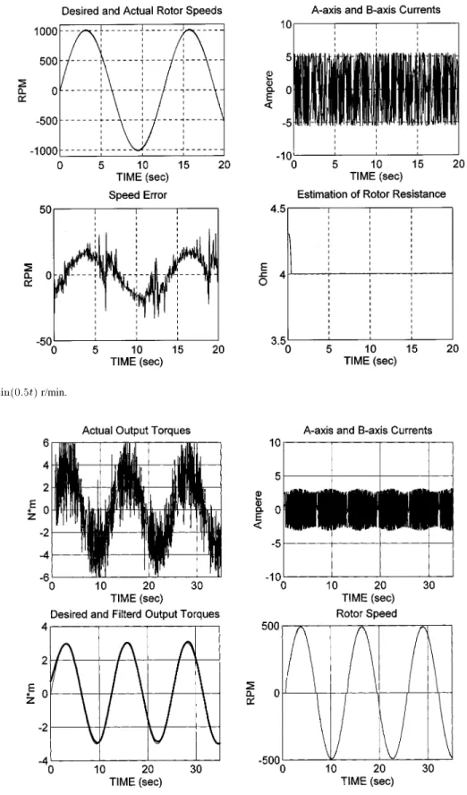
Fig. 3. ! = 1000 sin(0:5t) r/min.
Fig. 4. T = 3 sin(0:5t) N1m.
Before the theorem is presented, a useful working lemma will be introduced first, which helps to establish the fast speed con-vergence.
Lemma 2: Consider the following linear time-varying
equa-tion:
(24)
where , and is a bounded function, which
approaches 0 asymptotically. Then, approaches 0 asymp-totically.
Proof: Please refer to [15].
Theorem 2: Consider an induction motor whose dynamics
Fig. 5. Benchmark specification for simulation.
Fig. 6. Simulation of the benchmark test.
the desired rotor speed is a bounded, second-order continuously differentiable function and is defined in the following form:
Then, the rotor speed will approach asymptotically by the controller the same as that of Theorem 1.
Proof: Please refer to [15].
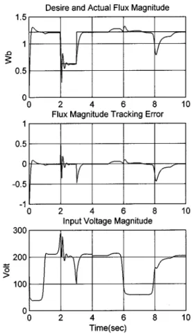
Fig. 7. Simulation of the benchmark test under the rotor resistance variation.
IV. RESULTS ANDDISCUSSIONS
A. Experiment Apparatus
The experiment consists of a Pentium PC, one power bipolar junction transistor (BJT) inverter with sinusoidal pulsewidth modulation (SPWM) which switches in 2 KHz, one 16-b D/A board, and a decoder board. A six-pole 1-hp three-phase induc-tion motor with a squirrel-cage rotor is used and is equipped with a 1024-pulse/rev encoder. The motor is manufactured by ELMA Motors Company with delta-connected stator, and the specifications are as follows:
rated power—0.75 KW; rated current—4 A; rated voltage—220 V; rated frequency—60 Hz; rated speed—1120 r/min; poles—six; ; ; mH; mH; mH; N m .
To demonstrate the performance of our controller persua-sively, we will make a variety of experiments on the induction motor. The test cases include speed control for desired (asym-totically) constant speed and desired sinusoidal speed, and torque control for desired constant torque. All the results are illustrated in Figs. 2–4. In Fig. 2, the desired rotor speed is
specifically given as r/min and, in
Fig. 3, the desired rotor speed is r/min
with the maximum tracking error 20 r/min at the positive and negative peak speeds. Both figures apparently demonstrate the satisfactory speed tracking performance. For torque control, the successful torque tracking is illustrated in Fig. 4.
B. Simulations with Benchmark Specification
We also perform computer simulations for the benchmark example. The rotor speed is required to change between these
values: , 0.1 , 0.25 , 1.5 during
s, where the r/min. The rotor flux is required
to change from to 0.5 when the rotor speed
is 1.5 , where Wb. The load torque is
0.5 at s and changes to 0.25 at s
where N m, and the rotor resistance variation is
30%. The benchmark specification is shown in Fig. 5. The benchmark assumptions are as follows.
B1) Measurable signals are the stator currents ( , ) and rotor speed .
B2) Load torque is constant, although unknown. B3) All parameters are known, but the rotor resistance
will change.
B4) Stator and rotor currents and stator voltages are con-strained by 12 A and 300 V.
B5) The system begins with all zero initial conditions. The simulation results for the speed tracking are shown in Figs. 6 and 7. In order to comply with the theory developed in this paper, especially the assumptions on the smoothness of the
desired speeds, we adopt a smooth function to approximate the step function so that the desired speed is continuously differen-tiable. One can find that the speed tracking is insensitive to the load torque variation. The speed tracking error will converge no matter what the desired values of the rotor flux norm and rotor resistance are. When the rotor resistance variation is considered, the error convergence for speed tracking will be slightly slower, which is shown in Fig. 7.
V. CONCLUSIONS
From the simulation and experiment results, we can make the following observations.
• The desired speed and torque trajectories can be assigned arbitrarily as long as they satisfy assumptions A6) and A4). • In addition to the speed and torque control, we are able to
control the flux magnitude as well.
• From the experiment results, we can see that the good tracking performance of the proposed servo controller will not be affected by the existence of the load torque. From (8), the error between and is dependent on the desired currents and the desired fluxes, which is directly related to and the desired flux magnitude by (10). Therefore, the convergence rate of the tracking may be different for different values of and . It is noteworthy that the estimation of rotor resistance will not approach the true value of the rotor resistance .
In this paper, we have successfully proposed a nonlinear adap-tive speed and torque servo controller, in which the rotor resis-tance is not required to be known exactly. We also give a rigorous proof of global stability without singularity and guarantee that the tracking error will converge to zero asymptotically.
REFERENCES
[1] M. Bodson, J. Chiasson, and R. Novotnak, “High-performance induction motor control via input–output linearization,” IEEE Contr. Syst. Mag., vol. 14, pp. 25–33, Aug. 1994.
[2] G. Espinosa and R. Ortega, “State observers are unnecessary for induc-tion motor control,” Syst. Control Lett., vol. 23, no. 5, pp. 315–323, 1993. [3] J. Hu and D. M. Dawson, “Adaptive control of induction motor systems despite rotor resistance uncertainty,” in Proc. American Control Conf., Seattle, WA, Jun. 1996, pp. 1397–1402.
[4] I. Kanellakopoulos, P. T. Krein, and F. Disilvestro, “Nonlinear flux-ob-server-based control of induction motors,” in Proc. American Control
Conf., Chicago, IL, June 1992, pp. 1700–1704.
[5] Z. Krzeminski, “Nonlinear control of induction motor,” in Proc. 10th
IFAC World Congr., Munich, Germany, 1987, pp. 349–354.
[6] P. C. Krause, Analysis of Electric Machinery. New York: McGraw-Hill, 1987.
[7] R. Kreshnen and F. C. Doran, “Study of parameter sensitivity in high-performance inverter-fed induction motor drive systems,” IEEE Trans.
Ind. Applicat., vol. IA-23, pp. 623–635, July/Aug. 1987.
[8] A. De Luca and G. Ulivi, “Design of an exact nonlinear controller for in-duction motors,” IEEE Trans. Automat. Contr., vol. 34, pp. 1304–1307, Dec. 1989.
[9] R. Marino, S. Peresada, and P. Valigi, “Adaptive input–output linearizing control of induction motors,” IEEE Trans. Automat. Contr., vol. 38, pp. 208–221, Feb. 1993.
[10] R. Marino, S. Peresada, and P. Tomei, “Adaptive output feedback control of current-fed induction motors,” in Proc. 12th IFAC World Congr., vol. 2, Sydney, Australia, July 1993, pp. 451–454.
[11] , “Adaptive observer-based control of induction motors with un-known rotor resistance,” in Proc. IEEE Conf. Decision and Control, Lake Buena Vista, FL, Dec. 1994, pp. 696–697.
[12] N. Mohan, T. M. Undeland, and W. P. Robbins, Power Electronics:
Con-verters, Applications, and Design. New York: Wiley, 1989. [13] R. H. Park, “Two-reaction theory of synchronous
machines—General-ized method of analysis—Part I,” AIEE Trans., vol. 48, pp. 716–727, July 1929.
[14] J.-H. Yang, W.-H. Yu, and L.-C. Fu, “Nonlinear observer-based adaptive tracking control for induction motors with unknown load,” IEEE Trans.
Ind. Electron., vol. 42, pp. 579–586, Dec. 1995.
[15] A.-M. Lee, L.-C. Fu, C.-Y. Tsai, and Y.-C. Lin, “Nonlinear adaptive speed and torque control of induction motors with unknown rotor resistance,” Dept. Elect. Eng., National Taiwan Univ., Taipei, Taiwan, R.O.C., Tech. Rep..
An-Ming Lee was born in Koashiung, Taiwan, R.O.C., in 1971. He received the B.S. degree in control engineering from National Chiao-Tung University, Hsin Chu, Taiwan, R.O.C., and the M.S. degree in electrical engineering from National Taiwan University, Taipei, Taiwan, R.O.C., in 1994 and 1996, respectively.
In 1996, he joined the Fine Mechanism Design Department, MIRL/ITRI, Hsin Chu, Taiwan, R.O.C., where he has been engaged in the development of high speed CD-ROM devices and digital camera systems. His research interests include adaptive control, nonlinear control, and analog circuits design.
Li-Chen Fu (S’85–M’88) was born in Taipei, Taiwan, R.O.C., in 1959. He received the B.S. degree from National Taiwan University, Taipei, Taiwan, R.O.C., and the M.S. and Ph.D. degrees from the University of California, Berkeley, in 1981, 1985, and 1987, respectively.
Since 1987, he has been a member of the faculty, and is currently a Professor in both the Department of Electrical Engineering and Department of Computer Science and Information Engineering, National Taiwan University. He also currently serves as the Deputy Director of the Tjing Ling Industrial Research Institute, National Taiwan University, and is an Associate Editor of Automatica and the Editor of the Journal of Control and Systems Technology. His research interests are adaptive control and system identification, nonlinear system control, robot motion planning, multi-sensing, control of robots, FMS scheduling, and neural networks for pattern recognition.
Dr. Fu received the Excellent Research Award for the period 1990–1993 and Outstanding Research Awards in 1994 and 1997 from the National Science Council, the Outstanding Youth Medal in 1991, the Outstanding Engineering Professor Award in 1995, and the Best Teaching Award in 1994 from the Min-istry of Education. He is a member of the IEEE Control Systems and IEEE Robotics and Automation Societies. He is also a Board Member of the Chinese Automatic Control Society and the Chinese Institute of Automation Technology.
Chin-Yu Tsai was born in Taipei, Taiwan, R.O.C., in 1975. He received the B.S. degree in control engineering from Chiao-Tung University, Hsin Chu, Taiwan, R.O.C., in 1997.
His research interests include nonlinear adaptive control, motor control, and real-time control applica-tions.
Yu-Chao Lin received the B.S. degree in control engineering from National Chiao-Tung University, Hsin Chu, Taiwan, R.O.C., and the M.S. degree from National Taiwan University, Taipei, Taiwan, R.O.C., in 1996 and 1998, respectively.
His research interests include nonlinear control system analysis, adaptive control, and motor control.