Hand-Eye Coordination for Visual Targets by Hebbian Learning Using Neural Networks

(1)

--Hand

-

Eye Coordination for Visual Targets

by

H

ebbian Learning Using Nelli

'

al Networks

Supervisor

:

B

e

rtram,

SHI

X

i

a

o

-

yu,

LI

,

Student 10: , Year 3,

Department of Electronic and Computer Engineering,

School of Engineering, Hong Kong Univ. of Science and Technology,

Abstract

We describe a robotic system consisting of a robotic arm and an active vision system. This work takes a bio-inspired approach that introduces a two-stage-neural-networks model for hand-eye coordination whose inputs are joint angles of the robotic arm and visual sensory signals. It's trained by unsupervised llebbian learning nile, and reward is given to strengthen the association between inputs. After learning these two stages alignments, experiments with the system show accurate hand-eye coordination for visual targets.

Supervisor Endorsement

Professor Bertram, S1-I [

~

Signature: ~

-1 ~

/./ /l

I

(2)

2

I. Introduction

Automatic robotics has been widely applied in many fields including manufacture industry, research, earth and space exploration, etc. The employment of robotics has significantly improved productivity, accuracy, endurance while fulfilled dangerous or inaccessible tasks. Research shows that more than 1 million industrial robots are working in factories worldwide in 2007, and that the personal and service robotic market will exceed 20 billion USD by 2010. With severe population ageing in near future, personal and service robots are being developed to perform regular housework for ageing people. In such situation, it requires robotics can not only perform the required task safely and accurately, but also handle much complex scenarios in real world. To properly handle unexpected changes, vision guidance is introduced to provide real time visual feedback and increase the flexibility and accuracy of robotics system. Considered as strategic development in the upcoming robotics market, vision-guided technique has been a hot topic in recent years. Among these most basic tasks, the hand-eye coordination has been drawn great attention by both neuroscience and robotic community.

A number of studies have investigated the hand-eye coordination or visually pointing by a robotic arm, e.g. [1][2][3]. Hashimoto, Kubota [4] propose control scheme for robotic manipulator by neural network that make use of direct image data without kinematics and geometry image processing. Salinas and Abbot [5] have shown that motor response can be correctly generated through the observation of random movements and correlation-based synaptic modification. This idea has been further elaborated to develop dynamical model for reaching task in [6]. Following this approach, Wang and Wu [7] use a Hebbian network to learn the alignment between sensory and motor maps.

The objective of this work is to perform accurate object tracking through hand-eye coordination. Different with previous work [7] that pointing by single glimpse, we develop two stages neural networks that adding active feedback of target and hand relation in the second stage. To improve performance in both stages, we introduce histogram equalization method to allocate neurons in each dimension. First stage neural network controls the end-effector (hand) to approach visual features defined as target by initial identification of sensory signals of target position. In the second stage, based on spatial relationship between hand and target seen in stereo camera, a fine-tone neural network is developed to control the hand to reach the target. Both stages of neural networks are trained based on Hebbian learning rule. After learning motion behavior of hand with corresponding visual information, the system can perform accurate target reaching through active visual guidance.

After a short introduction to system platform in Section II, visual tracking strategy is briefly described in Section III. Section IV presents the structures of two stage neural

(4)

4

network, neuron allocation method and learning algorithm. The experiments performed to validate this approach are discussed in Section V.

II. System Description

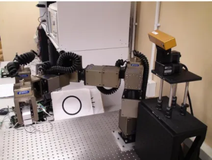
The system platform (Figure 1) consists of a robotic arm and a vision system to simulate hand-eye system of human. In the arm system, a seven Degree of Freedom (DoF) arm with a parallel gripper from SCHUNK that simulates human arm structure. In the vision system, a stereo camera named Bumble-bee from Point Grey that simulates human eyes is used to capture active image as visual input. The stereo camera is mounted on a pan-tilt unit from Directed Perception that simulates motion of head posture. Visual image processing, learning algorithms and arm and pan-tilt controls are implemented on a PC.

Figure 1 System platform

III. Visual Tracking Method

As a baseline visual behavior, the vision system maintains binocular fixation on the predefined target, e.g. red or blue light emitting diode (LED). The pure color LED provides a convenient and effective way to train the system by reducing uncertainty of target location in visual inputs. The input images are first filtered by Gaussian low pass filter of window size 5 by 5 to reduce noise from visual signals. Then an intensity threshold method is applied to estimate the target position by the region’s centroid. Based on the assumption that target positions in consecutive images are nearby, a local searching algorithm is implemented to reduce computation in comparison with full search method and meet the real time processing requirement (25Hz).

(5)

5

In order to maintain the fixation, the system updates pan and tilt angles of the pan-tilt unit. Based on the target position obtained from image processing, a pan-tilt control algorithm is implemented (simplified from work done in [8]). Denote the target position in left camera image is (x_left, y_left) and that in right camera image is (x_right, y_right) related to the center of the image. We could also obtain the camera setting Focal Length f (in pixels) and Baseline B (in centimeter). Thus, we could calculate 3D position (in centimeter) in relative to camera coordinate as follows:

Xc = x_left + x_right ∙ B 2 xleft − xright Y_c = yleft + yright ∙ B 2 x_left − x_right Z_c = f ∙ B x_left − x_right

By taking approximation, the transform between pan-tilt coordinate and camera coordinate can be neglect, thus we could calculate the changes in pan-tilt angles to maintain target in the binocular fixation.

Δθpan = − arctan X_c 𝑍_𝑐 Δθ_tilt = − arctan Yc 𝑋𝑐2+ 𝑌𝑐2

The system updates pan-tilt angles based on above algorithm so that the stereo camera keeps accurate tracking of the target. Updates occur every 40ms (25Hz).

IV. Neural Networks System

Based on biological research on cortical mechanism and human prehension, specifically, how infants learn hand-eye coordination in controlling limb. We believe infants learn hand-eye coordination through trial-error that strengthens the biological connection (inside cortex) between arm joint angles, head posture and spatial relation of hand and target. During the process of individual growing, we adapt changes in our physical structure and consistently learn, update cortex (our neuron network) and fulfill coordination task. Therefore, the two stage neural networks mimic such associations. As a fact, even adults couldn’t accurately grasp an object in space by glimpse. The pre-trained first stage neuron network cannot guarantee accurate coordination for the visual target. So our system establishes second stage learning scheme that trains the hand-target relation that both seen in vision. In this work, we move only the shoulder and elbow

(6)

6

joints of the arm, which are refer to as Joint 0 and Joint 1. Thus the end-effector moves along a 2D surface.

A. Architectures of two stage neural networks

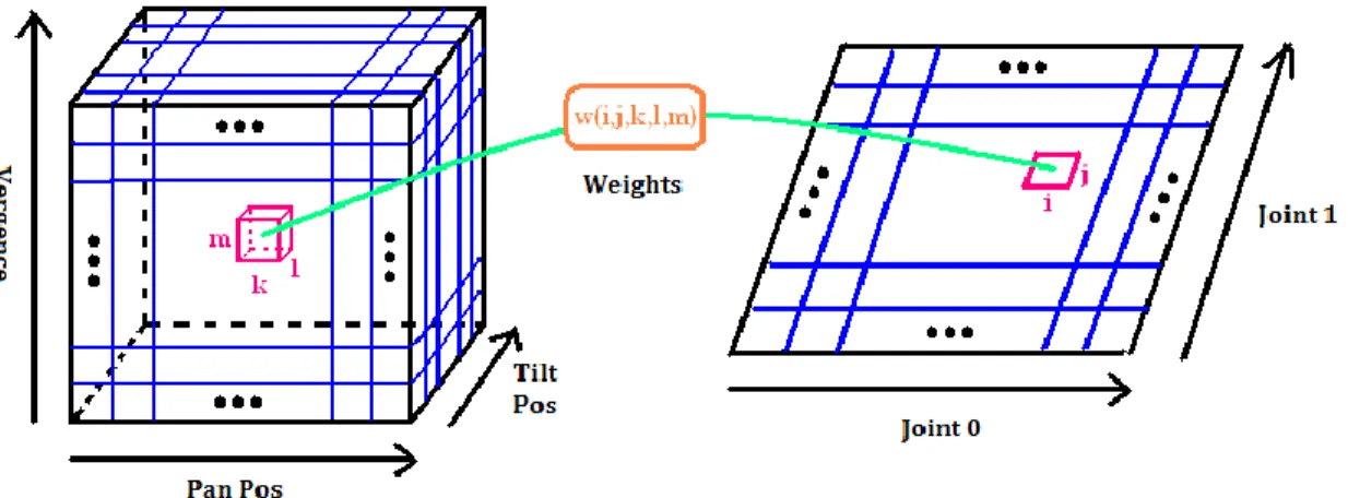
In first stage neural network, we use 10x10x10 arrays of neurons for sensory signals of pan position P_p, tilt position P_t and vergence P_v and 10x10 arrays of neurons for robotic arm joint angles θ0, θ1. Each neuron in 3D array of sensory inputs represents a

combination of three positions and that in 2D array of motor commands represents a combination of joint angles. By connecting neurons with activity strength (weight), the neural network is constructed as shown in Figure 2.

Figure 2 Architecture of first stage neural network

In order to accurately reach target, we introduce second stage neural network. It is implemented by similar structure as that in the first stage. From stereo vision geometry, the 3D position difference between target and hand can be calculated from pixel location of both objects in left and right camera images. To avoid uncertainty in non-linear mapping in geometry calculation, we directly use the pixel difference between them. Theoretically the difference in y axis should be identical. So the average of them dy (in pixel) is used as the first dimension. The other two dimensions of neurons are constructed from the difference in x axis from left and right camera (in pixel) respectively, denoted as dx_left, dx_right . In consistent with visual signals, we use 10x10 arrays of neurons for changes in robotic arm joint angles dθ0, dθ1. Therefore, when hand reaches the target, the

responses for both joint angles are zero and hand-eye coordination is fulfilled.

In the 2D arrays of arm commands for both neural networks, the distributed activity of each neuron is converted into a pair of commanded joint angles by the weighted average among all activity. Suppose the number of neurons in each dimension is N. Denote the activity of neuron at (i, j) by m_a(i, j) , where 0 ≤ i ≤ N − 1,0 ≤ j ≤ N − 1 and the

(7)

7

normalized center of that neuron by (x0,i, x1,j). The generated joint angles (C0, C1) are

given by C₀ = 1 M x0,i∗ 𝑚𝑎(𝑖, 𝑗) N−1 j=0 N−1 i=0 C1 = 1 M x1,j∗ 𝑚𝑎(𝑖, 𝑗) N−1 j=0 N−1 i=0 M = 𝑚𝑎(𝑖, 𝑗) N−1 j=0 N−1 i=0

Then the normalized joint angles are converted back to actual joint angles by linear scale and offset.

Each neuron in 2D arrays has different level of response when receiving external command of arm angles. The activity of each neuron pe(i, j) is assigned based on the

distance between external arm angles and angles represented by that neuron. We use Gaussian function to simulate the response intensity among neurons. Denote the external commands for arm angles after normalization by (e0, e1),

pe(i, j) ∝ ℕ (x0,i, x1,j) e0, e1 , σ2I2×2

where ℕ x m , C is a multi-dimensional Gaussian with mean m and covariance matrix C, I2×2 is the 2 by 2 identity matrix, σ2 is a positive constant that measures the spread of

activity in neighbor neurons.

Similarly, each neuron in 3D arrays of the sensory signals has different level of response when receiving actual sensory signal. Denote the activity of each neuron p_v(k, l, m), its center by (y_0,k, y_1,l, y_2,m) and the actual sensory signals after normalization by (v0, v1, v2),

pv(k, l, m) ∝ ℕ (y0,k, y1,l, y2,m) (v0, v1, v2), σ2I3×3

So the activity of neurons follows 3-dimensional Gaussian distribution. The actual activity of neuron p_e(i, j) and p_v(k, l, m) are normalized such that sum of all activity is constant.

B. Neuron Allocation

Involving complex forward/inverse kinematics and transformation between camera and arm, the transformation between motor and sensory signals cannot be roughly simplified as linear mapping. To address this complexity and improve the efficiency in neuron

(8)

8

1. Count number of samples c n that falls into the bin n which is equally located from 0 to 1 with size of _10N1 . Denote the total number of samples is CN, and c n for

0 ≤ n ≤ 10N − 1;

2. Denote the probability of an occurrence of each bin level as px n =c(n)_𝐶

𝑁 ;

3. Perform Equalization between these bins by using cumulative distribution function:

4. Record edges e_y(j) that the CDF of x surpluses each re-located level j

N :

ey 0 ≜ 0,

e_y j =_10Ni when cdf_x i ≥_Nj and cdf_x i − 1 <_Nj, where 1 ≤ j ≤ N. cdfx i = px j

i j=1

;

distribution, we implement histogram equalization method to re-allocate neuron in each dimension. As in our training phase, we could command the arm joints move in designed behavior with equally distributed over its range, so the histogram equalization method is applied to sensory signals for both stages.

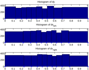
To illustrate the histogram equalization method in neuron allocation, we make use of the training data in the second stage. The histograms of dθ₀, dθ₁ and dy, dx_left, dx_right are shown below in Figure 3.

Figure 3 Histograms of motor and sensory signals after normalizing in range of [0,1]

The histogram equalization method in relocating neurons of sensory signals is designed as follows to map signal x to y:

0 0.1 0.2 0.3 0.4 0.5 0.6 0.7 0.8 0.9 1 0 50 100 150 200 Histogram of d₀ 0 0.1 0.2 0.3 0.4 0.5 0.6 0.7 0.8 0.9 1 0 50 100 150 200 Histogram of d₁ 0 0.1 0.2 0.3 0.4 0.5 0.6 0.7 0.8 0.9 1 0 200 400 Histogram of dy 0 0.1 0.2 0.3 0.4 0.5 0.6 0.7 0.8 0.9 1 0 200 400 Histogram of dx_left 0 0.1 0.2 0.3 0.4 0.5 0.6 0.7 0.8 0.9 1 0 200 400 Histogram of dx_right

(9)

9

The histogram of sensory signals after histogram equalization is shown below in Figure 4. We denote the center of each neuron as the average between its boundaries obtained from histogram equalization.

Figure 4 Histogram of sensory signals after equalization

C. Learning Rules

By bounding the synaptic weights, the Hebbian-based learning rule is implemented as a biologically plausible algorithm. During the training for first stage neural network, the vision system maintains tracking of the end-effector by adjusting pan, tilt position and vergence. So the activity of external arm angles affects that of sensory signals. During the training for second stage neural network, although the pan-tilt unit keeps stationary, the difference between target and hand position in visual coordinate is affected by the change in arm commands. In short, the activity of external inputs affects the activity of the sensory signals for both stages.

As two stage neural networks share similar structure, here we briefly illustrate that of first stage neural network. Denote the associativity (weight) between joint angles at neuron (i, j) and sensory signals at neuron (k, l, m) as W(i, j, k, l, m) as shown in Figure 2. The activity of neurons of arm joint angles is driven by both external arm commands and weighted response from sensory signals:

ma i, j = W i, j, k, l, m pv k, l, m N−1 m=0 N−1 l=0 N−1 k=0 + C ∙ pe i, j

where C is the training weight. When training, C is large to overrides the first term induced from sensory signals, and during evaluation, C is set to zero as we don’t have external signals. 0 0.1 0.2 0.3 0.4 0.5 0.6 0.7 0.8 0.9 1 0 200 400 Histogram of dy 0 0.1 0.2 0.3 0.4 0.5 0.6 0.7 0.8 0.9 1 0 200 400 Histogram of dx_left 0 0.1 0.2 0.3 0.4 0.5 0.6 0.7 0.8 0.9 1 0 200 400 Histogram of dx_right

(10)

10

The weight W(i, j, k, l, m) is learned via Hebbian learning rule. In each training set, the weight is updated to strengthen the connection of the strong activities between motor and sensory signals:

∆W i, j, k, l, m = η ∙ ma(i, j) ∙ pv(k, l, m)

where η is a positive learning rate. W(i, j, k, l, m) is viewed as the probability that sensory signals occur at neuron (k, l, m) when arm commands are at neuron (i, j). So, in each iteration, weight W is normalized for each possible configuration of arm commands.

V. Experimental Results and Comparisons

A. Training Procedure

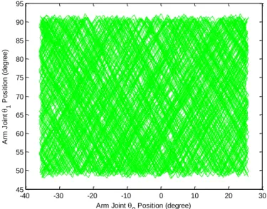
During the training for first stage neural network, the robotic end-effector holds a red LED as target. The stereo camera maintains target in its binocular fixation by pan-tilt control. The system is updated every 40ms. Arm motion is controlled within a defined range. To construct random and equally distributed movements for two joint angles, joint 0 is moved by constant speed and joint 1 is moved by random speed. The direction of either joints reverses when reaching its boundary. The trajectory of two joints is shown in Figure 5.

Figure 5 Trajectory of arm joint 0 and 1

We could observe that the 2D arrays of neurons are statistically equally distribution and fired. As discussed in previous section, the sensory signals (pan, tilt position and vergence) are not fully explored. By implementing histogram equalization, neurons of each dimension receive roughly same amount of trainings. The Hebbian learning algorithm described in previous section updates the connection between motor and

-40 -30 -20 -10 0 10 20 30 45 50 55 60 65 70 75 80 85 90 95 Arm Joint  0 Position (degree) A rm J o in t 1 P o s it io n ( d e g re e )

(11)

11

sensory signals. The weight is initially randomly assigned and normalized. After training for around 7,000 data sets (7,000 weight updates), it constructs stable weight between 2D neurons of arm joint angles and 3D neurons of sensory signals.

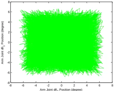
During the training for second stage neural network, the robotic end-effector holds a red LED as hand position. At initial state, the robotic arm is randomly moved in defined range, and the pan-tilt unit performs tracking to locate the red LED in its binocular fixation. The joint angles and visual position of red LED is recorded and this state is denoted as origin. Then the robotic arm is randomly moved in a local region and changes in both joints angle from origin is bounded in [−6, 6] degree range. The changes in the observed hand positions in stereo camera are also recorded to build up the association between two sets of signals. After training in one origin for 100 data sets, the robotic arm moves to another position and repeats above local training. After training for 45 different origins (4,500 weight updates), the trajectory of changes in joint angles is shown in Figure 6. Similarly, the training data span the 2D arrays of neurons.

Figure 6 Trajectory of arm joint 0 and 1

B. Testing Results

During the testing period, the external inputs will not be available, and we could simply set training weight C to be zero.

1. Evaluation of First Stage Neural Network

In order to evaluate the performance of first stage neural network, we keep the target at the hand and disable commanded signal to control joint angles. This allows us to move arm joints to difference positions while analyzing the generated motor signals from neural network. Figure 7 shows the comparision beween actual arm positions and

-8 -6 -4 -2 0 2 4 6 8 -8 -6 -4 -2 0 2 4 6 8 Arm Joint d 0 Position (degree) A rm J o in t d 1 P o s it io n ( d e g re e )

(12)

12

generated commands by fisrt stage neural network after training. Errors between corresponding signals are calculated by mean square error.

Figure 7 Comparision between actual arm commands (green marked) and generated neuron responses (red marked) in first stage neural network

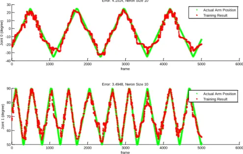
To futher illustrate the method of histogram equalization in neuron allocation, we also implement method that equally locate neuron in each dimension. Its performance is shown in Figure 8.

Figure 8 Comparision between actual arm commands (green marked) and generated neuron responses (red marked) in first stage neural network without Histogram Equalization

0 1000 2000 3000 4000 5000 6000 -40 -30 -20 -10 0 10 20 30 J o in t 0 ( d e g re e ) frame Error: 2.8903, Neron Size 10

Actual Arm Position Training Result 0 1000 2000 3000 4000 5000 6000 50 60 70 80 90 J o in t 1 ( d e g re e ) frame Error: 2.8301, Neron Size 10

Actual Arm Position Training Result 0 1000 2000 3000 4000 5000 6000 -40 -30 -20 -10 0 10 20 30 J o in t 0 ( d e g re e ) frame Error: 4.1514, Neron Size 10

Actual Arm Position Training Result 0 1000 2000 3000 4000 5000 6000 50 60 70 80 90 J o in t 1 ( d e g re e ) frame Error: 3.4948, Neron Size 10

Actual Arm Position Training Result

(13)

13

One wrong direction occurs when the generated signal from network is in different direction with that of the actual signal and the actual signal is significantly away from origin, e.g. 0.5 degree in our experiment. The wrong direction ratio is the ratio of number of wrong direction over total number of training set.

With the implementation of histogram equalization in neuron allocation, the performances of both joints are improved by 30.3% and 20.2% respectively. If we assume that the distributions of errors in two joints follow Gaussian distribution, then variances σ2_{for both joints are bounded in 3 degree. When we perform second stage}

neural network training with range of [-6, 6] degree from origin, it is expected to cover and improve errors in the range of ±3.5σ or equivalent 99.95% of the errors in first stage neural network.

2. Evaluation of Second Stage Neural Network

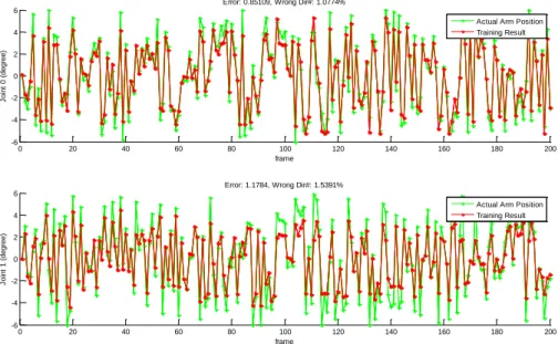
To analyzing the performance of second stage neuron network, we apply similar strategy as that in training, but disconnecting the generated arm commands by this network with the actual commands. After moving arm randomly to one location, the pan-tilt unit stops tracking and the system sets current stage as origin. Then the arm is controlled randomly move in that local region, and generated arm commands from this network are compared with actual positions (Figure 9):

Figure 9 Comparision between actual arm commands (green marked) and generated neuron responses (red marked) in second stage neural network

As second stage neural network is designed to generate on-line arm commands based on active sensory signals, we also compare the wrong direction ratio defined as follows:

0 20 40 60 80 100 120 140 160 180 200 -6 -4 -2 0 2 4 6 J o in t 0 ( d e g re e ) frame Error: 0.85109, Wrong Dir#: 1.0774%

0 20 40 60 80 100 120 140 160 180 200 -6 -4 -2 0 2 4 6 J o in t 1 ( d e g re e ) frame Error: 1.1784, Wrong Dir#: 1.5391%

(14)

14

The MSEs in this neuron network are around 1 degree for both joints, however, though on-line control, the error is expected to converge.

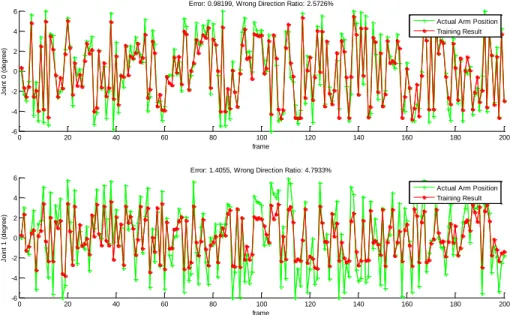
In this neural network, we also compare the performance of the network that uses equally spaced neuron allocation (Figure 10):

Figure 10 Comparision between actual arm commands (green marked) and generated neuron responses (red marked) in second stage neural network without histogram equalization

With the implementation of histogram equalization in neuron allocation, the performances of both joints are improved by 13.3% and 16.2% in MSE respectively and 58.1% and 67.9% in wrong direction ratio respectively. We notice that there is dramatic improvement in wrong direction ratio which emphasizes more on the stability of real time control. One plausible explanation is that through neuron re-allocation by histogram equalization, the dense region (around origin) is better clarified and the connection between 3D sensory signals and 2D arm signals is less ambiguity. In addition, the performance of joint 1 is better improved than that of joint 0. We speculate that due to the structure of robotic arm, by same range in joint angle, the sensory signals caused by joint 0 spread into a larger range than that caused by joint 1. When we perform histogram equalization, the center regions of sensory signals, affected by both joint 0 and 1, are better refined. Therefore, the effect of joint 1 is better represented in the network.

3. Evaluation of Merged Neural Networks

To evaluate the performance of two stage neural networks, we introduce two LEDs that blue one is randomly placed in space as target and red one is held by hand of the robotic arm. The vision system keeps on tracking the blue LED target and observes the hand position if it’s seen in camera. At first, we randomly place the target position in reachable space of hand. Then the system will first make use of first stage neural network to move

0 20 40 60 80 100 120 140 160 180 200 -6 -4 -2 0 2 4 6 J o in t 0 ( d e g re e ) frame

Error: 0.98199, Wrong Direction Ratio: 2.5726%

0 20 40 60 80 100 120 140 160 180 200 -6 -4 -2 0 2 4 6 J o in t 1 ( d e g re e ) frame

Error: 1.4055, Wrong Direction Ratio: 4.7933%

(15)

15

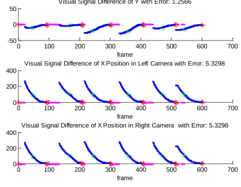
the arm approach the target. Once hand position is found in visual system, the system will switch to second stage neural network and move further closer towards the target. At the beginning of each test, two joints are setting to their minimum bounds respectively. The observed difference between hand and target from camera is shown below (Figure 11):

Figure 11 Performance of two-stage neural network model in visual difference, the magenta marked point indicates the hand position is not seen in stereo camera,

the green marked point indicates the start of second stage neural network and the red marked point indicates the end of one test

Define error as the difference between target and hand position in pixel when the system is stabilized (at the end of each test). Then we measure the MSE of each dimension. The results show that the pixel differences between target and hand position are within 10 pixels. In camera image, it usually takes more than 5x5 pixel size to represent one LED. By taking the centroid of the LED region, it is hard to further improve the performance. Besides, when two different color LEDs get close, the light color will be mixed thus it introduces more uncertainty in locating the actual position of hand and target from stereo camera.

To evaluate the generated joint positions by two stage neural networks and the joint positions to reach the target, we run another test that moves the arm randomly in space with red LED held in hand. Then we put the target (blue LED) as close as possible to the hand (red LED). Thus the current joint position of arm can be approximated as that of the

0 100 200 300 400 500 600 700 -50

0 50

frame

Visual Signal Difference of Y with Error: 1.2566

0 100 200 300 400 500 600 700 0

200 400

frame

Visual Signal Difference of X Position in Left Camera with Error: 5.3298

0 100 200 300 400 500 600 700 0

200 400

frame

(16)

16

corresponding target. Based on this approximation, we could evaluate both the performance in visual coordinates (Figure 12) and joint coordinates (Figure 13).

Figure 12 Performance of two-stage neural network model in visual difference, with similar color notation of Figure 11

Figure 13 Performance of two-stage neural network model in joint angles, with similar color notation of Figure 11

0 100 200 300 400 500 600 700 -50

0 50

frame

Visual Signal Difference of Y with Error: 2.0054

0 100 200 300 400 500 600 700 0

200 400

frame

Visual Signal Difference of X Position in Left Camera with Error: 10.8464

0 100 200 300 400 500 600 700 0

200 400

frame

Visual Signal Difference of X Position in Right Camera with Error: 10.8464

0 100 200 300 400 500 600 700 -40 -20 0 20 40

Joint 1 Position with Error 0.98394

frame 0 100 200 300 400 500 600 700 40 50 60 70 80

Joint 2 Position with Error 0.9408

(17)

17

From Figure 12 and 13, we notice that the performance of visual difference is slightly worse. And the estimated mean square errors of both joints are less than 1 degree. However as we cannot obtain the correct joint angles for that target, estimated errors could only illustrate relatively accurate performance of two stages neural networks.

VI. Conclusion

In this work, we have demonstrated a biologically plausible development of hand-eye coordination for visual target. The two stage neural networks are used to construct the connections between motor signals and sensory signals derived from stereo camera and pan-tilt unit. Histogram equalization method is applied in neuron allocation to maximize the connections between motor and sensory signals. After training both networks by Hebbian learning rule, the vision-guided reaching task is accurately achieved. Further work on this system includes deriving mathematical model for motor and sensory relationship and increasing the dimensionality of the system.

Reference

[1]. Kuperstein M. Neural model of adaptive hand-eye coordination for single postures. Science, vol. 239, no. 4845, pp.1308–1311, 1988.

[2]. T. Martinetz, H. Ritter, and K. Schulten. Three-dimensional neural netfor learning visuo-motor coordination of a robot arm. IEEE Transactions on Neural Networks, Vol. 1, pp.131-136, 1990.

[3]. M. Marjanovic, B. Scassellati, and M. Williamson. Self-Taught Visually-Guided Pointing for a Humanoid Robot. In Proceedings of the Fourth International Conference on Simulation of Adaptive Behavior, Sep. 1996.

[4]. H. Hashimoto, T. Kubota, W-C. Lo and F. Harashima. A Control Scheme of Visual Servo Control of Robotic Manipulators Using Artificial Neural Network. In Proc. IEEE Int. Conf. Control and Applications, pp. TA 3 6, 1989.

[5]. E. Salinas and L. F. Abbot. Transfer of Coded Information from Sensory to Motor Networks. Journal of Neuroscience, vol. 75, no. 10,pp.6461-647, Oct. 1995.

[6]. D. Caligiore, D. Parisi, and G. Baldassarre. Toward an integrated biomimetic model of reaching. In 6th IEEE International Conference on Development and Learning, pp.241-246, 2007.

[7]. Yiwen Wang, Tingfan Wu, Orchard, G., Dudek, P., Rucci, M., Shi, B.E.. Hebbian learning of visually directed reaching by a robot arm. Biomedical Circuits and Systems Conference, 2009. BioCAS 2009. IEEE , pp.205-208, 26-28 Nov. 2009.

[8]. Dzialo, Karen A., Schalkoff, Robert J.. Control Implications in Tracking Moving Objects Using Time-Varying Perspective-Projective Imagery. IEEE Transactions on Industrial Electronics, IE-33, Issue: 3, 1986, p247-253.