This article was downloaded by: [National Chiao Tung University 國立交通大學] On: 27 April 2014, At: 21:53
Publisher: Taylor & Francis
Informa Ltd Registered in England and Wales Registered Number: 1072954 Registered office: Mortimer House, 37-41 Mortimer Street, London W1T 3JH, UK
Production Planning & Control: The
Management of Operations
Publication details, including instructions for authors and subscription information:
http://www.tandfonline.com/loi/tppc20
Improving supply chain efficiency via option
premium incentive
Chi-Sheng Shi & Chao-Ton Su Published online: 15 Nov 2010.
To cite this article: Chi-Sheng Shi & Chao-Ton Su (2002) Improving supply chain efficiency via option premium incentive, Production Planning & Control: The Management of Operations, 13:3, 236-242, DOI: 10.1080/09537280110065508
To link to this article: http://dx.doi.org/10.1080/09537280110065508
PLEASE SCROLL DOWN FOR ARTICLE
Taylor & Francis makes every effort to ensure the accuracy of all the information (the “Content”) contained in the publications on our platform. However, Taylor & Francis, our agents, and our licensors make no representations or warranties whatsoever as to the accuracy, completeness, or suitability for any purpose of the Content. Any opinions and views expressed in this publication are the opinions and views of the authors, and are not the views of or endorsed by Taylor & Francis. The accuracy of the Content should not be relied upon and should be independently verified with primary sources of information. Taylor and Francis shall not be liable for any losses, actions, claims, proceedings, demands, costs, expenses, damages, and other liabilities whatsoever or howsoever caused arising directly or indirectly in connection with, in relation to or arising out of the use of the Content.
This article may be used for research, teaching, and private study purposes. Any substantial or systematic reproduction, redistribution, reselling, loan, sub-licensing, systematic supply, or distribution in any form to anyone is expressly forbidden. Terms & Conditions of access and use can be found at http://www.tandfonline.com/page/terms-and-conditions
Improving supply chain e ciency via option
premium incentive
CHI-SHENG SHI and CHAO-TON SU
Keywords stochastic demand, return policy, decentralized
control, centralized control, option premium, Pareto e ciency
Abstract. This study considers a supply chain, including one
manufacturer and one retailer, in which stochastic demand and return policy is focused upon. When each site aims to maximize its individual pro®tability, decentralized control may arise in the system. From the overall system’s point of view, the decen-tralized supply chain will not be as e cient as the cendecen-tralized one. Various studies have attempted to resolve the ine ciency of supply chains. However, such studies have focused on the optimization from retailer’s perspective only and thus ignored manufacturer’s interest. This study emphasizes manufacture’s self-interested situation and determines optimal production quantity. Furthermore, it will contribute to decentralized con-trol with the retailer o ering option premium. It is also demon-strated that the Pareto e ciency can be attained in the supply chain by employing the option premium incentive.
1. Introduction
Consider a supply chain including one manufacturer and one retailer. The system serves an uncertain market demand that is the general experience in the competitive environment. That is, the actual demand at a speci®c due date is unpredictable. Therefore, the manufacturer’ s quantity setting at the outset of produc-tion is quite important. If the determined quantity is too large, the deterioration cost might be enormous. However, shortage will occur if the determined quan-tity is insu cient. On the other hand, due to the ben-e®t from the manufacturer’ s overproductio n at no immediate cost, the retailer has the incentive to initi-ally over forecast but eventuiniti-ally purchase smaller quantity. The manufacturer must in turn anticipate
Authors: Chi-Sheng Shi, and Chao-Ton Su, Department of Industrial Engineering and
Management, National Chiao Tung University, 1001 Ta Hsueh Road, Hoinchu, Taiwan, E-mail: ctsu@cc.nctu.
Chi-Sheng Shi is currently a doctoral candidate in industrial engineering at National Chiao Tung University, Taiwan. His present research interests are in the ®eld of production/inventory control and production management.
Chao-Ton Su is Professor of the Deparment of Industrial Engineering and Management, National Chiao Tung University, Taiwan. He received his PhD from University of Missouri-Columbia, USA. His current research activities include quality engineering, production manage-ment and neural networks in industrial applications. Dr Su has published articles in Computers and
Industrial Engineering, Computers in Industry, International Journal of Industrial Engineering, Internaitonal Journal of Production Research, International Journal of Operations & Production Management, International Journal of Production Economics, Production Planning & Control, Integrated Manufacturing Systems, Opsearch, Quality Engineering, Quality and Reliability Engineering International, International Journal of Quality and Reliability Management, International Journal of Quality Science, International Journal of Systems Science, IEEE Transactions on Components, Packaging, and Manufacturing Technology, European Journal of Operational Research, IIE Transactions, Total Quality Management, Industrial Management and Data Systems.
Production Planning & Control ISSN 0953±7287 print/ISSN 1366±5871 online # 2002 Taylor & Francis Ltd http://www.tandf.co.uk/journals
DOI: 10.1080/0953728011006550 8
the outcome, particularly when a return policy is in place. If the manufacturer and the retailer make deci-sions independently, a rational manufacture r will deter-mine the production quantity by maximizing his pro®t within both production cost and wholesale price. Thus, the market often su ers the shortage. If the manu-facturing lead time is su ciently short, the retailer can match the demand by employing backup but at an extra premium to compensate for overtime produc-tion cost. If the lead time fails to permit backup, then the retailer and manufacturer should absorb the market loss. In this study, the lead time is assumed to be insu cient for backup to occur. This results in an ine cient supply chain and is referred to as decen-tralized control (cf. Iyer and Bergen 1997, Lee and Whang 1999, Tsay 1999). Tsay (1999) proposed an e ciency benchmark deemed central control, where the retailer and manufacture r are coordinate d by a single entity and therefore the system is able to deliver the maximum expected pro®t.
Various studies have attempted to remedy ine cient supply chains, as will be noted in Section 2. In this study, the manufacturer’ s self-interest is emphasized and the production quantity optimized. Furthermore, it is demonstrated that in comparison to centralized model, decentralized control causes an insu cient sup-ply chain. That is, implementation of a centralized model results in extra pro®t and Pareto e ciency. However, in the centralized model, production quan-tity must be increased, which in turn decreases the manufacturer’ s pro®t. Hence, without compensation, a manufacturer will have no incentive to accept such a contract. As a result, it is proposed that a retailer should o er an option premium to induce a manufac-turer to increase the production quantity. This, while not a ecting the manufacturer, will increase the retai-ler’s pro®t, and thus result in extra pro®t as a whole. Restated, an option premium incentive is proposed to resolve the dilemma of a decentralized supply chain. This study also demonstrates that when the option premium incentive is applied to a decentralized supply chain, the Pareto e ciency obtained will equal that of a centralized model.
The rest of this paper is organized as follows: section 2 reviews relevant literature. In section 3, a brief descrip-tion of the decentralized model is provided. Secdescrip-tion 4 characterizes the centralized scenario with conjoining of the retailer and the manufacturer by a single entity. In section 5, the option premium incentive is proposed to improve the e ciency of a supply chain. In section 6, a numerical example is presented to illustrate the e ective-ness of the proposed approach. Section 7 summarizes the conclusions of this study.
2. Literature review
Recently, many researchers have modelled the decen-tralized scenario. Fisher and Raman (1996) analysed a quick response (QR) environment and demonstrated a two-stage ordering process, which could reduce both stockout and markdown costs by reducing the lead time su ciently to allow a portion of production to be com-mitted after observation of the initial demand. Iyer and Bergen (1997) considered a similar environment. They demonstrate d that after QR, a retailer’s order could decrease, whereas, under the same conditions, a manu-facturer might be negatively in¯uenced. Thus, to com-pensate the manufacturer, three tools are employed, including requirement for better service to customers, increase in wholesale price, and volume commitment. Tsay (1999) modelled the decentralized situation by `quantity ¯exibility’ coupled with the customer’s commit-ment to purchase no less than a certain percentage and the supplier’s guarantee to deliver up to a certain percen-tage. The decentralized models mentioned above attempt to remedy the problems underlying decentralized con-trol. However, they emphasize the retailer’s interests and disregard those of the manufacturer.
Duenyas et al. (1993) illustrated the relationship between production quota and card setting. They pro-posed an algorithm to calculate card counts as well as the optimal quota for a constant work in process (CONWIP) system. Duenyas et al. (1997) determined the production quota by assuming that both demand and production are uncertain. Also, they considered overtime production. The costs included in their model are regular time pro-duction, ®xed cost of overtime, variable overtime costs, and holding cost. By optimizing the manufacturer’s position, these studies determined production quota. However, they neglect to consider the system decentrali-zation that would result.
Padmanabhan and Png (1997) studied the strategic e ect of the return policy on retailers competition and highlighted its pro®tability implications to manufac-turers. Eppen and Iyer (1997) investigate d the backup in which a vendor agrees to retain a predetermined per-centage of the retailer’s forecasted quantity. Based on the agreement, the retailer is allowed to buy the backup items with no additional premium but must pay a pen-alty for the items not taken from backup. Emmons and Gilbert (1998) developed a model incorporating the retailer’s interests with the policy decisions of the manu-facturer. This con®rmed that both the manufacturer and the retailer could bene®t from a return policy under speci®c conditions. The above investigations provide a profound insight into understanding of the return policy. Furthermore, most of them conclude that due to the return policy, a retailer will order a greater quantity,
Improving supply chain e ciency 237
thus bene®ting the manufacturer. However, this should assume that the manufacturer has an unlimited supply capacity. In fact, a pro®t-maximizing manufacture r will not expect unlimited production, as it occurs with the risk of overproduction .
Gurnani and Tang (1999) analysed the demand forecast updating scenario with a retailer who, prior to a single selling season, had two instants to order seasonal products from a manufacturer. To determine the pro®t-maximizing ordering strategy of both instants, the retailer had to evaluate the tradeo between a more accurate forecast and a potentially higher unit cost. Parlar and Weng (1997) considered a model of joint coordination between a ®rm’s manu-facturing and supply departments with two runs. The result con®rmed that a supply department would cure additional reserved material for the second pro-duction, for which a higher price would be charged, if the co-operation were optimal. Otherwise, a supply department should only order the amount of requested material for an initial production run. Weng (1997) considered a manufacturer±distributor supply chain, which encountered price sensitive stochastic demand. The decision variables in this instance were the distri-butor’s order quantity (which equalled the manufac-turer’s production since the production was make-to-order), retail sale price, as well as the manufacturer’s wholesale price. Notably, the model presumed that any excessive demand must be satis®ed completely through a second, more costly production run. The above studies provide the same scenario in which a retailer, with an additional fee, can take advantage of backup when the demand exceeds the order quantity. Additionally, a second run is available only if the man-ufacturer’s production lead time is su ciently short. However, in many industries, the lead time is often over one year. Hence, the setting of the manufacturer’s production quantity is rather important.
3. Problem description
The problem is described as follows. In response to a given wholesale price and production cost, the manufac-turer determines the production quantity by realizing the company’s best interest (i.e. maximizing pro®t). During the selling season, the retailer sells the items in the market at a constant retail price. At the end of the season, the retailer returns unsold items to the manufacturer for full credit.
The relevant assumptions are twofold. (a) The distri-bution of market demand is available. Although this is a simpli®cation, it is known that the distribution can be found by analysing history data. (b) Under the
circum-stance with return policy, prior to the selling season, the retailer makes commitment in terms of order quantity and wholesale price, and at the end of the season, is allowed to return unsold items. Pasternack (1985) assumed two forms of return policy, which include partial credit to the retailer for all unsold items and full credit for the return of a certain portion of the original order. To simplify it, the retailer is assumed to have received full credit for all unsold items in this study. Thus, it is possible to focus on the model to be described, which deals with a pro®t-oriented manufacturer.
To construct the model, the relevant notation is stated as follows:
w wholesale price per item
w0 baseline wholesale price per item, that is, the price when no option premium is o ered ¢w option premium, the di erence between w and
w0, de®ned as…w ¡ w0†
m production cost per item
p retail price per item
u salvage value per item
s shortage cost per item
D market demand, stochastic variable
Q production quantity of manufacture r
Qd production quantity of decentralized model
Qc production quantity of centralized model
F…¢† distribution function of the market demand
f…¢† density function of the market demand
To assure internal consistency, the cost parameters follow some straightforward assumptions:
(a) p > w0> m > 0, (b) u < m, (c) s > 0.
2.1. Manufacturer’s pro®t function
The manufacturer’ s pro®t can be expressed as whole-sale revenue minus production costs plus salvage value. Notably, wholesale revenue only counts sold items because unsold items are returned with full credit.
ºmˆ w0Min…Q ; D† ¡ mQ ‡ u…Q ¡ D†‡ …1† Take expectation for all possible demand, then the man-ufacturer’s average pro®t can be written as:
E…ºm† ˆ w0EfMin…Q ; D†g ¡ mQ ‡ uE…Q ¡ D†‡ …2† Di erentiation of equation (2) yields the following ®rst-order condition:
@ @Q E…ºm† ˆ w0 @ @QfE…D† ¡ E…D ¡ Q † ‡g ¡ m ‡ u @ @QE…Q ¡ D† ‡ ˆ w0…1 ¡ F…Q †† ¡ m ‡ uF…Q † ˆ …w0¡ m† ‡ …w0¡ u†F…Q † ˆ 0 …3† or it can be rewritten as F…Q † ˆ …w0¡ m†=…w0¡ u† …4† Di erentiating equation (3) yields the second-order con-dition.
¡…w0¡ u† f …Q † µ 0 …5†
Hence, the second-order condition is satis®ed and
Qdˆ F¡1f…w0¡ m†=…w0¡ u†g is the manufacturer’s optimal production quantity.
2.2. Retailer’s pro®t function
The retailer’s pro®t can be expressed as revenue minus wholesale cost and goodwill loss. Notably, wholesale cost only counts sold items because unsold items can be returned for full credit.
ºrˆ …p ¡ w0† Min…Q ; D† ¡ s…D ¡ Q †‡ …6† Take expectation for all possible demand, then the re-tailer’s average pro®t becomes:
E…ºr† ˆ …p ¡ w0†EfMin…Q ; D†g ¡ sE…D ¡ Q †‡ …7† Di erentiation of equation (7) yields the following ®rst-order condition:
…p ‡ s ¡ w0†…1 ¡ F…Q †† ˆ 0 …8† It concludes that the retailer’s optimal ordering quantity is in®nite. Restated, the retailer hopes the manufacturer produces as many as possible so that shortage costs can be reduced signi®cantly. Furthermore, the retailer does not need to worry about ordering too much because unsold items can be returned for full credit.
If the manufacturer and the retailer make decisions independently, a rational manufacturer will determine the optimal production quantity by maximizing the pro®t. Since backup is prohibited in this study, once the production quantity is determined, regardless of shortage during a selling season, the retailer cannot acquire any extra quantity. Explicitly the shortage does not a ect the manufacturer but only matters to the retai-ler. Thus, the retailer encounters a great potential risk that is a shortage might destroy business viability. The situation mentioned above is also referred to as decentra-lized dilemma. If the pro®ts of the manufacturer and the
retailer are considered together, the quota ascertained in the model will not allow for too much shortage to occur. This is called a centralized scenario. The next section attempts to model the centralized scenario.
4. Centralized model
Let ºJ be the joint pro®t of the manufacturer and the
retailer, which can be written as ºJˆ ºr‡ ºm;
or
ºJ ˆ p Min…Q ; D† ¡ mQ ‡ u…D ¡ Q †‡¡ s…D ¡ Q †‡
…9† Take expectation for all possible demand, the manufac-turer average pro®t is:
E…ºJ† ˆ p Min E…Q ; D† ¡ mQ ‡ uE…D ¡ Q †‡
¡ sE…D ¡ Q †‡ …10†
Di erentiation of equation (10) yields the following ®rst-order condition:
…p ‡ s ¡ m† ¡ …p ‡ s ¡ u†F…Q † ˆ 0 …11† or rewritten as
F…Q † ˆ …p ‡ s ¡ m†=…p ‡ s ¡ u† …12† The second-order condition is produced by di erentiat-ing equation (11).
¡…p ‡ s ¡ u† f …Q † µ 0 …13† Therefore, the second-order condition is satis®ed and
Qc ˆ F¡1f…p ‡ s ¡ m†=…p ‡ s ¡ u†g is the system’s
opti-mal production quantity. Proposition 1
Joint pro®t of the centralized model is higher than that of the decentralized model.
As the objective of the centralized model is to maxi-mize the joint pro®t, this proposition is self-explana-tory. Therefore, the optimal joint pro®t of the centralized model is always higher than or equivalent to that of the decentralized model. Furthermore, once the optimal quota within the decentralized model is ascertained to be di erent from that within the central-ized one, the centralcentral-ized model dominates the decen-tralized model. Compare equations (12) and (4), the di erence of their optimal quota is apparent. So the centralized model dominates the decentralized model, or restated, extra pro®t results in the centralized model.
Improving supply chain e ciency 239
Proposition 2
The manufacturer’s pro®t of the centralized model is less than that of the decentralized one.
The objective of the decentralized model is to maxi-mize the manufacturer’ s pro®t, so that when optimum, the manufacturer’ s pro®t of the decentralized model is always higher than or equivalent to that of the centra-lized model. Furthermore, once the optimal quota within the centralized model di ers from that within the detralized one, the decendetralized model dominates the cen-tralized model. Proposition 1 con®rms that the optimal quota between two models is distinct, therefore, when the centralized model is implemented, the manufacturer’s pro®t decreases.
Proposition 3
The retailer’s pro®t of the centralized model is higher than that of the decentralized one.
From proposition 1, when optimum the joint pro®t of the centralized model is higher than that of the decen-tralized one. In addition, from proposition 2, the manu-facturer’s cost of the centralized model is less than that of the decentralized model. Thus, it is explicit that the retailer’s pro®t of the centralized model is higher than that of the decentralized one.
Proposition 4
The manufacturer’ s production quantity of the centra-lized model is greater than that of the decentracentra-lized situa-tion.
This proposition is proven by comparing Qdˆ
F¡1f…w0¡ m†=…w0¡ u†g and Qcˆ F¡1f…p ‡ s ¡ m†=
…p ‡ s ¡ u†g. Since p > w0 based on the assumption, and
F¡1…¢† is a monotonous increasing function, then
Qc> Qd can be concluded.
Proposition 5
Pareto e ciency is attained in the centralized model. A feasible allocation x is a Pareto e cient allocation if there is no feasible allocation xtsuch that all agents prefer
xt to x (cf. Varian 1984). There is no feasible production quantity where the manufacture r and the retailer are at least both well o and at least one of them is strictly better o . That is, if such a quantity exists, then the joint pro®t of the centralized model can be improved. However, the joint pro®t of the centralized model is max-imized in the supply chain. As a result, it can be
con-cluded that Pareto e ciency is attained in the centralized model.
The above propositions verify that when the centra-lized model is implemented, the manufacturer’s pro®t decreases, while both the retailer’s pro®t and the joint pro®t increase. Notably, the retailer’s pro®t increases more than the manufacturer’ s pro®t decreases, therefore, the manufacturer-retaile r system will yield extra overall pro®t. Furthermore, it is demonstrated that implementa-tion of the centralized model results in Pareto e ciency. However, problems still exist. If the manufacturer accepts a centralized model contract, it means that he must produce more but earn less. It is clear that unless compensated by the retailer, the manufacturer will not accept such a contract. This will be considered in the next section.
5. Cooperative model employing option premium as an incentive
In this section, it is proposed that the retailer employ an option premium as an incentive, so that the manufac-turer is motivated to accept the contract. Furthermore, it will determine the amount of the option premium that the retailer should o er. Also, production quantity in such a situation will be determined.
Let the option premium be ¢w that is de®ned as (w¡ w0), and ºm…Qd† be the pro®t function before the
option premium. After the option premium, the manu-facturer’s pro®t function can be expressed as ºm…Q †. If
the manufacturer’ s pro®t after option premium is not less than that of the decentralized model, the motivation to accept the contract of the centralized model will exist. Equation (14) expresses such a situation, where Qd is
the optimal production quantity of the decentralized model.
ºm…w; Q † ¡ ºm…w0; Qd† ¶ 0 …14†
For simplicity, let equation (14) equal zero, which implies that after option premium, the manufacturer’s pro®t is equal to that of the decentralized model. After solving equation (14), the reaction function of the man-ufacturer is as follows:
wˆfºm…Qd† ‡ mQ ¡ uE…Q ¡ D† ‡g
E…Min…Q ; D†† …15†
Furthermore, to determine the ordering quantity, the retailer will maximize pro®t under the reaction function, which is expressed in the following:
Max E…ºr† ˆ …p ¡ w†EfMin…Q ; D†g ¡ sE…D ¡ Q †‡
s:t: wˆfºm…Qd† ‡ mQ ¡ uE…Q ¡ D† ‡g
EfMin…Q ; D†g …16†
Di erentiation of equation (16) yields the following ®rst-order condition:
…p ‡ s ¡ m† ¡ …p ‡ s ¡ u†F…Q † ˆ 0 …17† It is evident that equation (17) is equivalent to equation (11). Thus, the ordering quantity determined herein is equal to that of the centralized model (i.e. Qc).
Substitute Qc into equation (15), the optimal wholesale
price w can be ascertained and option premium ¢w is obtained by…w ¡ w0†.
Proposition 6
Through the employment of option premium as an incentive, the manufacturer’s pro®t will not decrease compared with that of the decentralized model, whereas will increase compared with that of the centralized model. Meanwhile, the retailer’s pro®t will increase com-pared with that of the decentralized model, whereas will decrease compared with that of the centralized model. Furthermore, Pareto e ciency is also attained herein.
Based on equation (14), the manufacturer’s pro®t is equivalent to that of the decentralized model. From pro-position 2, the manufacturer’ s pro®t of the decentralized model is higher than that of the centralized one. Therefore, it can be concluded that the manufacturer’s pro®t herein is larger than that of the centralized model. Since option premium paid by the retailer is equivalent to the amount received by the manufacturer, therefore the joint pro®t of the manufacturer and the retailer will be also equivalent both before and after option premium. Thus, proposition 1 is also correct here. From proposition 1, extra pro®t exists within the centralized model. When the manufacturer’s pro®t equals that of the decentralized situation, it is explicit that the retailer’s pro®t will increase in comparison with that of the decentralized model. However, since the manufacturer’s pro®t herein is larger than that of the centralized model, the retailer’s pro®t will decrease in comparison with that of the cen-tralized model. Finally, Pareto e ciency is attained, because the joint pro®t after option premium is equiva-lent to that of the centralized model.
6. Numerical illustration
To illustrate the e ectiveness of the co-operative model, the decentralized control from previous literature is solved by the proposed approach. This problem
origi-nates from Tsay (1999). Tsay assumed that market demand is uniformly distributed within [0, 100]. He also assumed pˆ 15, w0ˆ 10, m ˆ 6, u ˆ 3. Here, it is assumed sˆ 3 in the retailer’s parameters.
First, the decentralized model is solved. The optimal quota which manufacturer produces is 57.14. Notably, every individual cost and the total pro®t are computed when the optimal quota is substituted into the manufac-turer’s pro®t function. Furthermore, with this quota, the retailer’s cost is also computed. Table 1 illustrates the results.
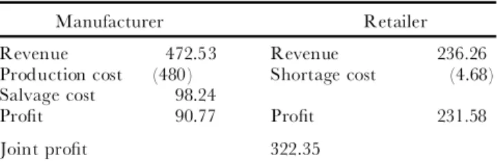
Then, the centralized model is solved. The optimal quota is 80. Notably, it is greater than that of the decen-tralized model (i.e. 57.14). When the option quota is substituted into the pro®t function of both the retailer and the manufacturer, every individual cost and the total pro®t are again computed. Table 2 illustrates the results. It shows that the retailer’s shortage cost decreases, but the manufacturer’s production and salvage costs increase here. As a result, the retailer’s pro®t increases, but here the manufacturer’ s pro®t decreases in compar-ison with that of the decentralized model. Moreover, the joint pro®t is 322.35, which increases by about 12.7% in comparison with that of the decentralized model.
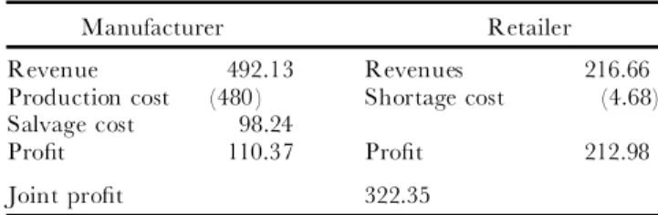
Finally, the co-operative model is solved. The optimal quota of 80 is the same as it is in the centralized model. When the optimal quota is substituted into the pro®t function of both the retailer and the manufacturer, every individual cost and the total pro®t are computed. The wholesale price can be solved as 10.41, thus option premium ¢w, 0.41, is obtained. That is, the retailer should o er an option premium, 0.41 per item to induce the manufacturer to increase the production quantity
Improving supply chain e ciency 241
Table 1. Results obtained from the decentralized model.
Manufacturer Retailer
Revenue 402.57 Revenue 201.28
Production cost (342.84) Shortage cost (25.67)
Salvage cost 50.64
Pro®t 110.37 Pro®t 175.61
Joint pro®t 285.98
Table 2. Results obtained from the centralized model.
Manufacturer Retailer
Revenue 472.53 Revenue 236.26
Production cost (480) Shortage cost (4.68)
Salvage cost 98.24
Pro®t 90.77 Pro®t 231.58
Joint pro®t 322.35
from 57.14 to 80. The results are illustrated in table 3, which shows that due to the option premium, the man-ufacturer’s pro®t, 110.37, equals that of the decentralized model. However, the retailer’s pro®t, 212.98, is higher than that of the decentralized model. Restated, it is increased by approximatel y 21.3%. In addition, the joint pro®t, 322.35, is equivalent to that of the centralized model.
7. Conclusions
The decentralized dilemma within a supply chain has been discussed. Stochastic demand and return policy are included in the model. Furthermore, the decentralized e ect within a supply chain has been revealed, as well as the decision policies of the retailer and the manu-facturer modelled. The retailer hopes the manumanu-facturer produce as many as possible, thereby reducing the cost of shortage due to the return policy. However, if the manu-facturer and the retailer make decisions independently, a rational manufacturer will determine the optimal pro-duction quantity by maximizing pro®t.
It has been proven that when a retailer and a manu-facturer are conjoined by a single entity, the system can attain the Pareto e ciency or centralization. Within the centralized model, the manufacturer must produce a greater amount, but earn less. Therefore, unless compen-sated, the manufacturer will not have the incentive to accept this type of contract. It is therefore proposed that the retailer should o er an option premium to induce the manufacturer to increase production quantity.
It has been demonstrate d that when the retailer o ers the manufacturer an option premium, the system can be Pareto e cient, and thus remedy the ine ciencies caused by decentralized control within a the system.
References
Duenyas, I., Hopp, W. J., and Spearman, M. L., 1993, Characterizing the output process of a CONWIP line with deterministic processing and random outages. Management
Science, 39(8), 975±988.
Duenyas, I., Hopp, W. J., and Bassok, Y., 1997, Production quotas as bounds on interplant JIT contracts. Management
Science, 43(10), 1372±1386.
Emmons, H., and Gilbert, S. M., 1998, Note: the role of returns policies in pricing and inventory decisions for catalogue goods. Management Science, 44(2), 276±283.
Eppen, G. D., and Iyer, A. V., 1997, Backup agreements in fashion buying ± the value of upstream ¯exibility. Management
Science, 43(11), 1469±1484.
Fisher, M., and Raman, A., 1996, Reducing the cost of demand uncertainty through accurate response to early sales. Operations Research, 44(1), 87±99.
Gurnani, H., and Tang, C. S., 1999, Note: optimal ordering decisions with uncertain cost and demand forecast updating.
Management Science, 45(10), 1456±1462.
Iyer, A. V., and Bergen, M. E., 1997, Quick response in manufacturer-retailer channels. Management Science, 43(4), 559±570.
Lee, H., and Whang, S., 1999, Decentralized multi-echelon supply chain: incentives and information. Management
Science, 45(5), 633±640.
Palar, M., and Weng, Z. K., 1997, Designing a ®rm’s coordi-nated manufacturing and supply decisions with short product life cycles. Management Science, 43(10), 1329±1344.
Padmanabhan, V., and Png, I. P., 1997, Manufacturer’s returns policies and retail competition. Management Science,
16(1), 81±94.
Pasternack, B. A., 1985, Optimal pricing and returns policies for perishable commodities. Marketing Science, 4, 166±176. Tsay, A. A., 1999, The quantity ¯exibility contract and
sup-plier-customer incentives. Management Science, 45(10), 1339± 1358.
Varian, H. R., 1984, Microeconomic Analysis, 2nd edn. (New York: W. W. Norton).
Weng, Z. K., 1997, Pricing and ordering strategies in manu-facturing and distribution alliances. IIE Transactions, 29(8), 681±692.
Table 3. Results obtained from the co-operative model.
Manufacturer Retailer
Revenue 492.13 Revenues 216.66
Production cost (480) Shortage cost (4.68)
Salvage cost 98.24
Pro®t 110.37 Pro®t 212.98
Joint pro®t 322.35