TFCS Selection Algorithms in the Mac Functionality of 3GPP

全文

(1)Name of Workshop: Computer Networks Title of the Paper: TFCS Selection Algorithms in the Mac Functionality of 3GPP Authors: Jian-Liang Lin,. Sheng-Tzong Cheng. and Chun-Yen Wang,. ,. Department of Computer Science and Information Engineering, National Cheng Kung University, Tainan, Taiwan. Email: p7888110@sparc1.cc.ncku.edu.tw Tel: 06-2757575 ext. 62529 Fax: 06-2747076. Contact Author: Jian-Liang Lin Abstract:. Transfer of mobile users’ data by means of sharing the finite radio bandwidth becomes more and more popular today. However, due to the increasing of the number of mobile users day by day, the lack of bandwidth is more serious. This paper investigates the Transport Format Combination Set (TFCS) selection problem in 3GPP and proposes effective methods for TFCS selection to dynamically map logical channels with vary data bit rate on-demand to transport channels so as to utilize the finite bandwidth. The methods of selection demonstrate the feasibility and efficiency by simulation.. Keywords: 3GPP, UE, Mac, TFCS, First Fit, Best Fit, and Dynamic Fit.

(2) TFCS Selection Algorithms in the Mac Functionality of 3GPP1 Jian-Liang Lin,. Sheng-Tzong Cheng. and Chun-Yen Wang,. ,. Department of Computer Science and Information Engineering, National Cheng Kung University, Tainan, Taiwan. Email: p7888110@sparc1.cc.ncku.edu.tw. Abstract Transfer of mobile users’ data by means of sharing the finite radio bandwidth becomes more and more popular today. However, due to the increasing of the number of mobile users day by day, the lack of bandwidth is more serious. This paper investigates the Transport Format Combination Set (TFCS) selection problem in 3GPP and proposes effective methods for TFCS selection to dynamically map logical channels with vary data bit rate on-demand to transport channels so as to utilize the finite bandwidth. The methods of selection demonstrate the feasibility and efficiency by simulation.. 1. The work is sponsored by the Institute of Information Industry under the contract of 91-C-33..

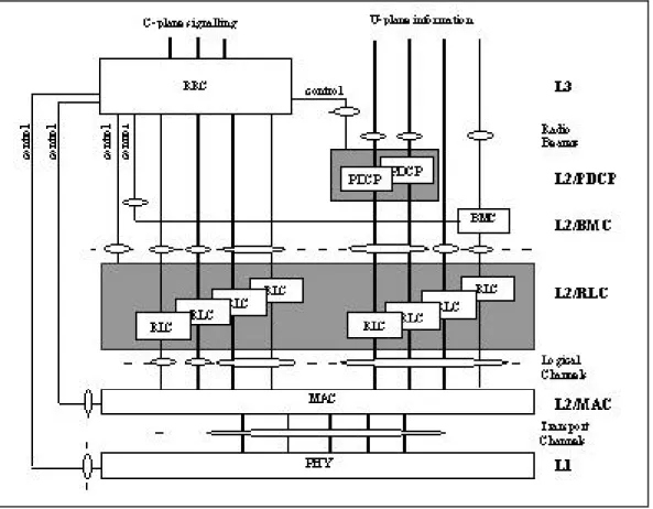
(3) 1 Introduction Data transmission on wireless and mobile devices will become a necessary part of every kind of applications in the near future. Mobile users share the limited bandwidth to transmit their information between each other. In order to utilize the air resource, technologies newly developed such as IMT-2000 (International Mobile Telephony 2000) supports variable bit rate to offer bandwidth on demand. During the uplink in IMT-2000, each mobile client who sends his own data in logical channel must map to transport channel at MAC layer. Mapping logical channel to transport channel of different transport format will consume different transmission power and occupy different bandwidth. Therefore, how to map the logical channel to a transport channel of suitable transport format from the predefined set of transport formats according to the total buffer size of logical channel will become an important part of the radio resource management now. In this paper, we propose three kinds of TFCS (Transport Format Combination Set) selection methods and each of them consists of two steps, assignment step and selection step. The first step is used to decide how much data of each logical channel can be transmitted in the next TTI for each TFC if we choose it to transmit, while the second is responsible to select a more suitable TFC according to the results from assignment step. The radio interface can be separated into the following three layers: the physical layer (layer 1), the data link layer (layer 2) and the network layer (layer 3). At Figure 1, Layer 2 can be split into four sublayers: Medium Access Control (MAC), Radio Link Control (RLC), Packet Data Convergence Protocol (PDCP) and Broadcast/Multicast Control (BMC). Between these layers, one of the MAC functions is the selection of appropriate transport format for each transport channel depending on instantaneous date rate of logical channels. That’s the reason that our TFCS selection functionality is located in MAC layer. We use the simulation to compare the performance of our methods and the others. Our experimental results confirm that our methods often have good quality and speed. Between these assignment algorithms, we prefer to adopt a dynamic_fit assignment algorithm. On one hand it can save more execution time, and on the other hand the selected TFC using dynamic_fit assignment algorithm often has lower bit rate so as to economize total transmitted power and decrease the possible interference. The rest of his paper is organized as follows. In Section 2, we describe the general concepts about the transport format combination set. In Section 3, we propose our two-phase TFC selection methods. In Section 4, we conduct a few experiments for the estimation of the performance of our TFC assignment algorithm. Finally, we conclude our result in section 5..

(4) Figure 1: Radio Interface protocol Architecture. 2 Background (The General Concepts of TFCS) In this section, we introduce some definitions and terms generally about the transport channels that are used in this paper. More detailed descriptions are defined in [1]. 2.1 Transport Block This is the basic unit exchanged between L1 and MAC, for L1 processing. Layer 1 adds a CRC for each Transport Block. 2.2 Transport Block Set This is defined as a set of Transport Blocks, which are exchanged between L1 and MAC at the same time instance using the same transport channel. 2.3 Transport Block Size This is defined as the number of bits in a Transport Block. The Transport Block Size is always fixed within a given Transport Block Set.(i.e., the size of all Transport Blocks within a Transport Block Set are equally.) 2.4 Transport Block Set Size This is defined as the number of bits in a Transport Block Set. 2.5 Transmission Time Interval This is defined as the inter-arrival time of two continuous Transport Block Sets, and is the.

(5) periodicity at which a Transport Block Set is transferred by the physical layer on the radio interface. It is always a multiple of the minimum interleaving period (e.g. 10ms, the length of one Radio Frame). The MAC delivers one Transport Block Set to the physical layer every TTI. DCH1. Transport Block. Transport Block Transmission Time Interval. DCH2. Transport Block Transport Block. Transport Block Transport Block. Transport Block. Transport Block. Transport Block. Transmission Time Interval. DCH3. Transport Block Transport Block Transport Block. Transport Block. Transport Block. Transport Block. Transport Block. Transport Block. Transport Block. Transmission Time Interval. Figure 2: example of data transmission on Transport Channel. Figure 2 shows an example the data transmission on three parallel Transport Channels by Transport Block Sets at certain time instances. Each Transport Block Set consists of a number of Transport Blocks. The Transmission Time Interval, i.e. the time between consecutive deliveries of data on the same Transport Channel, is also illustrated. 2.6 Transport Format This is defined as a format used for the delivery of a Transport Block Set during a Transmission Time Interval on a Transport Channel. The Transport Format is constituted of two parts – one is dynamic part and the other is semi-static part. Attributes of the dynamic part are: -. Transport Block Size;. -. Transport Block Set Size;. -. Transmission Time Interval (optional dynamic attribute for TDD only);. Attributes of the semi-static part are: -. Transmission Time Interval (mandatory for FDD, optional for the dynamic part of TDD NRT bearers);. -. error protection scheme to apply:. -. type of error protection, turbo code, convolutional code or no channel coding;. -. coding rate;.

(6) -. static rate matching parameter;. -. size of CRC.. EXAMPLE: Dynamic part: {320 bits, 640 bits}, Semi-static part: {10ms, convolutional coding only, static rate matching parameter = 1}.. Due to the semi-static part is often invariant, so it would be better to omit it in the following example. 2.7 Transport Format Combination The layer 1 multiplexes one or several Transport Channels, and there exists a list of transport formats (Transport Format Set) of all Transport Channels which are applicable. Nevertheless, at a given point of time, not all combinations may be submitted to layer 1 but only a subset of the Transport Format Combination. This is defined as an authorised combination of currently valid Transport Formats that can be submitted simultaneously to the layer 1 for transmission on a Coded Composite Transport Channel of a UE, i.e. containing one Transport Format from each Transport Channel. EXAMPLE: DCH1: Dynamic part: {20 bits, 20 bits} Semi-static part: {10ms, Convolutional coding only, static rate matching parameter = 2}; DCH2: Dynamic part: {320 bits, 1 280 bits} Semi-static part: {10ms, Convolutional coding only, static rate matching parameter = 3}; DCH3: Dynamic part: {320 bits, 320 bits} Semi-static part: {40ms, Turbo coding, static rate matching parameter = 2}.. 2.8 Transport Format Combination Set This is defined as a set of Transport Format Combinations on a Coded Composite Transport Channel. EXAMPLE: -. dynamic part:. -. combination 1: DCH1: {20 bits, 20 bits}, DCH2: {320 bits, 1280 bits}, DCH3: {320 bits, 320 bits};. -. combination 2: DCH1: {40 bits, 40 bits}, DCH2: {320 bits, 1280 bits}, DCH3: {320 bits, 320 bits};. -. combination 3: DCH1: {160 bits, 160 bits}, DCH2: {320 bits, 320 bits}, DCH3: {320 bits, 320 bits}.

(7) -. semi-static part:. -. DCH1: {10ms, Convolutional coding only, static rate matching parameter = 1};. -. DCH2: {10ms, Convolutional coding only, static rate matching parameter = 1};. -. DCH3: {40ms, Turbo coding, static rate matching parameter = 2}.. The Transport Format Combination Set controlled by MAC. However, the assignment of the Transport Format Combination Set is done by L3(RRC). When mapping data onto L1, MAC needs to choose one Transport Format Combination from the Transport Format Combination Set. Since the difference between the Transport Format Combinations is only the dynamic part, it is in fact only the dynamic part that MAC has any control over. Note that a Transport Format Combination Set doesn’t need to contain all possible Transport Format Combinations but only the allowed combinations that are included. Thereby a maximum total bit rate of all transport channels of a Code Composite Transport Channel can be set appropriately. That can be achieved by only allowing Transport Format Combinations for which the included Transport Formats (one for each Transport Channel) do not correspond to high bit rates simultaneously. The selection of Transport Format Combinations can be seen as a fast part of the radio resource control. The dedication of these fast parts of the radio resource control to MAC, close to L1, means that the flexible variable rate scheme provided by L1 can be fully utilized. These parts of the radio resource control should be distinguished from the slower parts, which are handled by L3. Thereby the bit rate can be changed very fast, without any need for L3 signaling. This paper investigates this problem and proposes an effective way of TFCS selection to dynamically vary data bit rate on demand so as to fully utilize the finite bandwidth. We will introduce three TFCS selection methods in the next section. 2.9 Transport Channel Reconfiguration As for the transport channel reconfiguration, this is done by sending a Transport Channel Reconfiguration message from the RRC layer in the network to its peer entity. This message contains the new transport format set and a new transport format combination set. On the contrary, a congestion situation occurs and allowed transport format combinations are restricted temporarily by sending a Transport Format Combination Control message from the network to the UE. Further, after a while when the congestion is resolved a new Transport Format Combination Control message is sent to the UE from the RRC layer in the network to recover the Transport Format Combination.. 3 Problem definition and Solution With the general TFCS concepts described above, now we can define the problem as: Given a TFCS with K TFCs, and the priority of each logical channel. How to choose a suitable TFC.

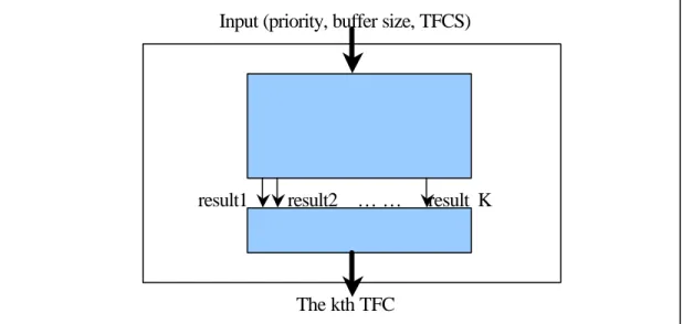
(8) according to the buffer size of each logical channel in RLC? In order to solve this problem, we offer a solution with good performance. In our basic idea, we are able to select a most suitable TFC if we can realize the result of each TFC when we choose it. Therefore, we construct our algorithm consisting of two phases, assignment phase and selection phase (see Figure 3). The first step, assignment phase, is used to decide how much data of each logical channel can be transmitted in the next TTI for each TFC we chose to transfer. The second step, selection step, is responsible to select a more suitable TFC according to the results from assignment step using some compare index. Input (priority, buffer size, TFCS). Assignment result1. result2 … …. result K. Selection The kth TFC Figure 3: TFC selection flow chart. Parameter. Summary. M K. The number of logical channels The number of TFCs. N. The number of transport channels in each TFC. L P[i]. The set of all logical channels The priority of ith logical channel. TrCH. The set of all transport channels. Bsize[i] BS[k][j]. The buffer of logical channel i in RLC The transport block size of jth transport channel in kth TFC. BSS[k][j]. The transport block set size of jth transport channel in kth TFC. D[k][i]. The transmitted data size of the logical channel i, if we select kth TFC. Table1: Parameters. The parameters that we will use in this paper are described in Table1 above. 3.1. Assignment Algorithm Here we describe the details of three kinds of assignment algorithms: (1) first fit, (2) best.

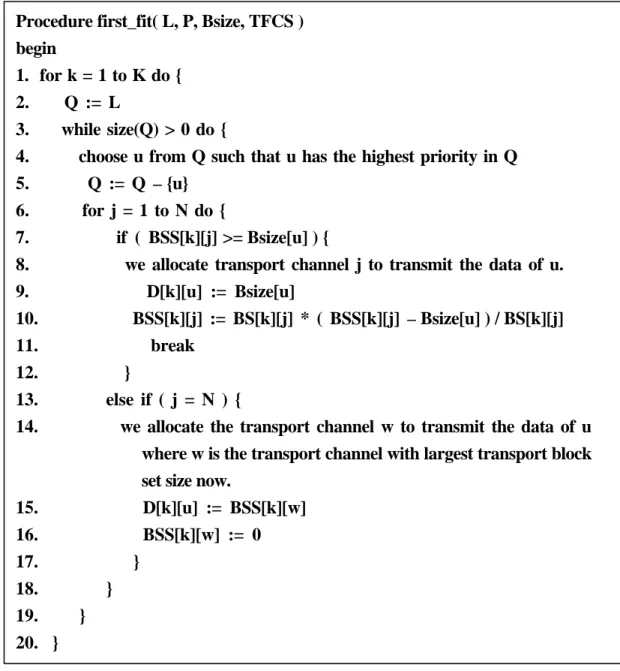
(9) fit and (3) dynamic fit. As we mentioned earlier, the input parameters to our assignment algorithm are the priority P[i] and the buffer size Bsize[i] of each logical channel in the set L and the TFCS including all TFCs we can choose in the present time. The outputs of the assignment algorithms are K results and each represents the transmitted data size of every logical channel (i.e., D[k][i]) transmitted by the TFC that we choose. That is to say, we have to calculate the most transmitted data size of all logical channel transferred by each TFC depending on the three kinds of different assignment algorithm. 3.1.1 Principals of Assignment Before we present our assignment algorithms, we prefer to describe assignment principals first. Now we gather those principals defined in 3GPP Technical Specification as follows: [P1]. The data of each logical channel can only be transmitted by not more than one transport channel. [P2] Each transport block can only transmit the data of one logical channel. [P3] The data of the logical channel with high priority have to be transmitted as much as possible. Based on these principals, we can realize the constraints on the assignment algorithm. For example, suppose that we allocate a transport channel to transmit a certain logical channel’s data, but the transport block set size of the transport channel is not large enough to carry all the logical channel’s data. Due to the first assignment principal constraint, we cannot assign another transport channel to transmit the remainder data of the logical channel. Besides that, take figure 7 for example, suppose that we now allocate transport channel v to transmit the data of the logical channel u that occupy only three transport block and still have 200 bits empty space. Because of the second assignment principal constraint, we cannot carry another logical channel’s data in the same transport block. However, we can allocate the remainder transport block to transmit another logical channel’s data.. 3.1.2. First fit. In this subsection, we describe the details of our first_fit algorithm (see Figure 4). We have known that in our assignment algorithm we have to calculate the most transmitted data size of each logical channel for each TFC. Hence, for each logical channel we would like to allocate the first transport channel whose block size is large enough to transmit all the data of the logical channel in our first fit assignment algorithm. In addition, based on the third assignment principal we would like to transmit more data for each higher priority logical channel. Therefore, we will allocate the transport channel from the higher priority logical channel first..

(10) Figure 4. First_fit algorithm. Procedure first_fit( L, P, Bsize, TFCS ) begin 1. for k = 1 to K do { 2. Q := L 3. while size(Q) > 0 do { 4. choose u from Q such that u has the highest priority in Q 5. Q := Q – {u} 6. for j = 1 to N do { 7. if ( BSS[k][j] >= Bsize[u] ) { 8. we allocate transport channel j to transmit the data of u. 9. D[k][u] := Bsize[u] 10. BSS[k][j] := BS[k][j] * ( BSS[k][j] – Bsize[u] ) / BS[k][j] 11. break 12. } 13. else if ( j = N ) { 14. we allocate the transport channel w to transmit the data of u where w is the transport channel with largest transport block set size now. 15. D[k][u] := BSS[k][w] 16. BSS[k][w] := 0 17. } 18. } 19. } 20. } First_fit procedure: For each logical channel, we require to allocate a transport channel to transmit its data (step 3). Initially, we desire to satis fy the previous third assignment principal so we have to assure that the data in the buffer of higher priority logical channels can be transmitted as much as possible. Thus, in Step 4, we permit the higher priority logical channel picking the transport channel first. And then, if we can find a transport channel whose transport block set size is larger than the buffer size of this logical channel then we’ll allocate this transport channel to transmit the data of the logical channel (see step 8). Therefore, the data size that can be transmitted in the next TTI of this logical channel is equal to the buffer size of this logical channel (step 9). And there are (BSS[k][j] – Bsize[u]) / BS[k][j] blocks remainder in this transport channel (step 10). On the other ha nd, if there is no transport channel whose transport block set size is large enough to transmit all the data of this logical channel (step 13) then we’ll.

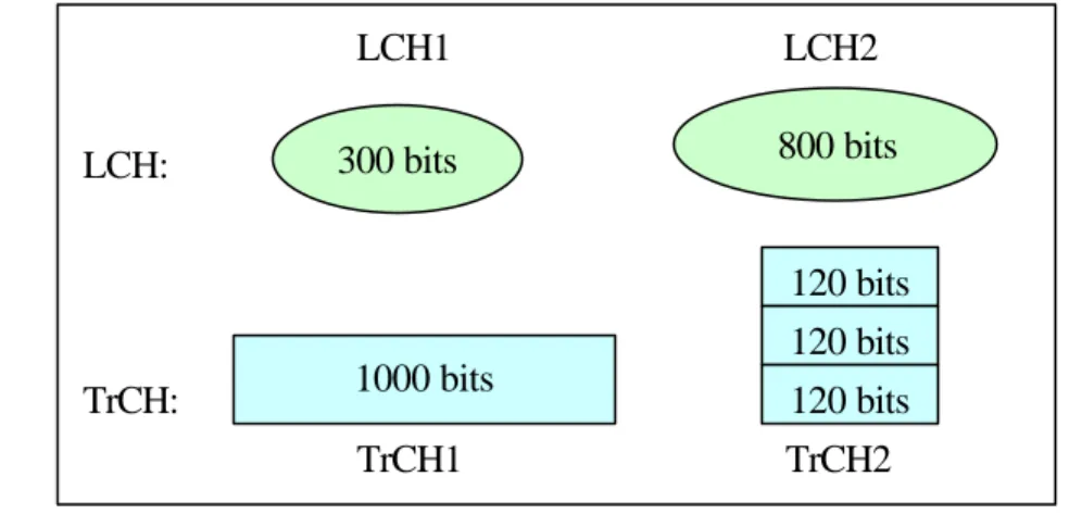
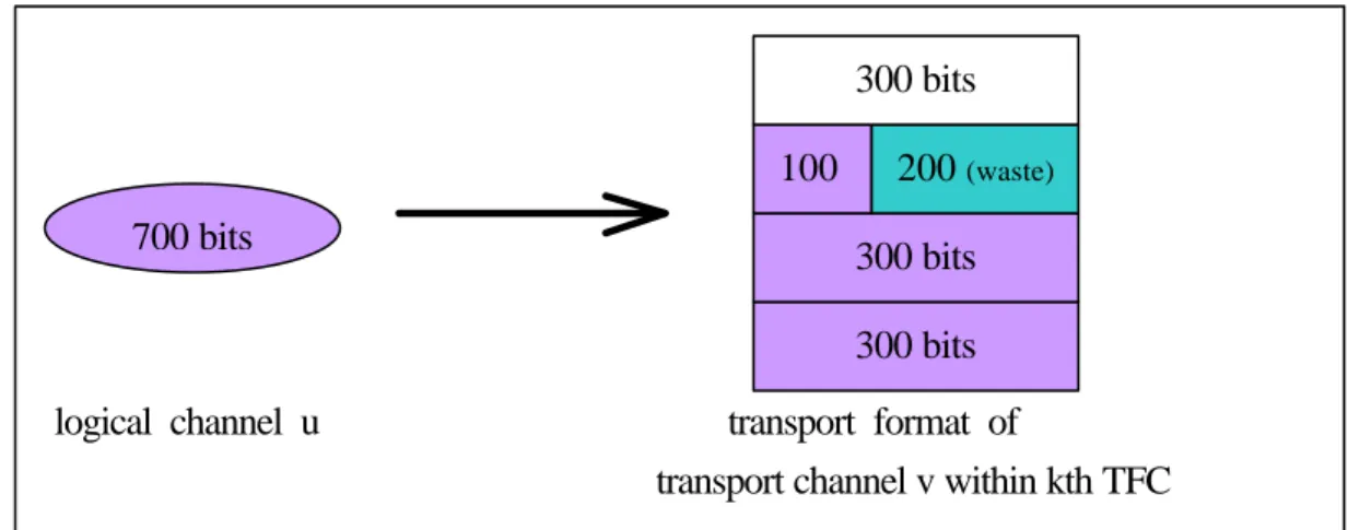
(11) allocate the transport channel whose block set size is largest now to transmit the logical channel’s data (step 14). Hence the data size that can be transmitted in the next TTI of this logical channel is equal to the block set size of the transport channel. And so there is no transport block remainder in this transport channel. In this way, all the results of each TFC when we choose it can be generated. 3.1.3 Best fit The previous first fit algorithm only takes the logical channel’s priority into consideration. Each logical channel just select the first transport channel whose transport block set size is large enough to transmit all the data of the logical channel. Unfortunately, this may result in a troublesome outcome because of the second assignment principal [P2]. Let’s consider the following condition: as shown in figure 5, suppose that there are two logical channels, LCH1 and LCH2, whose buffer size are 300 bits and 800 bits respectively. Between them, the priority of LCH1 is higher than that of LCH2. Assume that there is a TFC consisting of two transport channels with transport format TCH1: {1000bits, 1000bits} and TCH2: {120bits, 360bits}. According to the first_fit assignment algorithm, we will get the following result: i). We allocate TCH1 to transmit the 300 bits data of the LCH1.. ii). We allocate TCH2 to transmit the 360 bits data of the LCH2 while there is still 800 - 360 = 440 bits remainder.. However, if we allocate TCH2 to transmit the LCH1’s data and allocate TCH1 to carry the LCH2’s data, then there is no data remainder.. LCH:. TrCH:. LCH1. LCH2. 300 bits. 800 bits. 1000 bits TrCH1. 120 bits 120 bits 120 bits TrCH2 Figure 5: an example. In order to decrease the occurrence of the above situation, we propose another assignment algorithm named Best fit. Best fit strategy is based on the greedy algorithm skill to select a local optimal transport channel for each logical channel. Our basic idea of best fit is to find a less waste transport channel according to each logical channel’s buffer size..

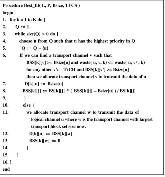
(12) Procedure Best_fit( L, P, Bsize, TFCS ) begin 1. for k = 1 to K do { 2. Q := L 3. while size(Q) > 0 do { 4. choose u from Q such that u has the highest priority in Q 5. Q := Q – {u} 6. If we can find a transport channel v such that BSS[k][v] >= Bsize[u] and waste( u, v, k) <= waste( u, v’ , k) for any other v’∈ TrCH and BSS[k][v’] >= Bsize[u] then we allocate transport channel v to transmit the data of u 7. D[k][u] := Bsize[u] 8. BSS[k][j] := BS[k][j] * ( BSS[k][j] – Bsize[u] ) / BS[k][j] 9. } 10. else { 11. we allocate transport channel w to transmit the data of logical channel u where w is the transport channel with largest transport block set size now. 12. D[k][u] := BSS[k][w] 13. BSS[k][w] := 0 14. } 15. } 16. } end Figure 6: Best_fit algorithm. Best_fit procedure: In order to follow the third assignment principal, we would like to enable the data in the buffer of higher priority logical channels can be transmitted as much as possible. Hence we imitate the first_fit method, in Step 4 we admit the higher priority logical channel choosing the transport channel first. After that, we define a subprocedure, waste(u, v, k), used to calculate the waste data size when we allocate transport channel v to transmit the data of the logical channel u (step 6). Take figure 7 for example, suppose that we now have a logical channel u with 700 bits data in its buffer and a transport channel v with four transport blocks whose size is 300 bits. It is easy to demonstrate that if we allocate transport channel v to transmit the 700 bits data of the logical channel u then it’ll take three blocks of v to transmit all the data and waste 200 bits.

(13) space within them and there is still one transport block remainder. Therefore we define the waste(u, v, k) value is 200 bits. That is to say, waste(u, v, k) is equal to 0 if Bsize[u] % BS[k][v] is equal to 0 else waste(u, v, k) is equal to BS[k][v] – ( Bszie[u] % BS[k][v] ) (refer to figure 8). 300 bits 100 700 bits. 200 (waste) 300 bits 300 bits. logical channel u. transport format of transport channel v within kth TFC Figure 7: example of internal fragmentation. As we mentioned earlier, for each logical channel we wo uld like to find a less waste transport channel to transmit its data. Thus, in step 6 we scan all the transport channel and estimate the waste space size; in the end we’ll assign the transport channel with least waste to transmit the data. If we can find such a transport channel then we’ll allocate this transport channel to transmit the data of the logical channel (see step 6). Therefore, the data size that can be transmitted in the next TTI of this logical channel is equal to the buffer size (step 7). Then there will be (BSS[k][j] – Bsize[u]) / BS[k][j] blocks remainder in this transport channel (step 8). On the other hand, if there is no transport channel whose transport block set size is larger than this logical channel then we’ll allocate the transport channel whose block set size is largest now to transmit the data (step11). Hence the data size that can be transmitted in the next TTI of this logical channel is equal to the block set size of the transport channel (step 12). And so there is no transport block remainder in this transport channel (see step 13). In this way, all the results of each TFC when we choose it are able to be generated. Procedure waste(u, v, k) Begin 1. if BSS[k][v] < Bsize[u] then return ∞ 2. if ( Bsize[u] % BS[k][v] = 0 ) then return 0 3. else return BS[k][v] – (Bsize[u] % BS[k][v]) end Figure 8: waste procedure.

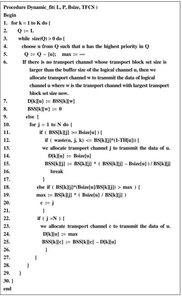
(14) 3.1.4. Dynamic fit. Although the effectiveness of best_fit can be much better tha n that of first fit, best_fit takes much time for each logical channel to find a less waste transport channel as it have to calculate each transport channel’s waste value for each logical channel. That’s the motive we propose the dynamic fit assignment algorithm. We would like decrease the execution time of the best fit by sacrificing a little bit its effectiveness in our dynamic fit assignment algorithm. For each logical channel, we would like to allocate the transport channel whose waste value is tolerable to transmit the logical channel’s data in our dynamic fit assignment algorithm. Thus we give each logical channel a tolerable waste value T[u] where T[u] is a decimal between 0 and 1. And then we will allocate the first transport channel whose block set size is larger than the buffer size of the logical channel and waste value divide its transport block size is less than the T[u] value. However, when there is no transport channel satisfying the above condition, that is to say no matter which transport channel we select, it will result in a large amount of waste space. So as to avoid the situation, we prefer to preserve the last transport block and only allocate the full- utilized transport block to transmit rather than transmitting all the data in the buffer of the logical channel. We favor to adopt the variable TH[u] which equal to 1-T[u] rather than adopting the variable T[u] in the following of this paper. Take figure 7 for example, suppose that the threshold TH[u] is 0.5 and we have known that the waste value of the transport channel v is 200 bits. It is over the tolerance value, thus we continue to check the next transport channel. Nevertheless, if there is no transport channel whose waste value is tolerate threshold, we will find the transport channel with maximum full- utilized transport blocks size to transmit. For example, the full- utilized transport blocks size of the transport channel v in figure 5 is 600 bits. Dynamic_fit procedure: By the same token, we would like to allocate a transport channel for each logical channel to transmit its data. Therefore, it is similar to the above assignment algorithm from step 1 to step 8 in our dynamic fit assignment algorithm. And then in step 11 and step 12, we check each transport channel whose block set size is larger enough to transmit all the data of the logical channel whether its waste size is tolerable. If the waste size of the transport channel is tolerable, then we allocate this transport channel to transmit directly and clearly the data size that can be transmitted in the next TTI of this logical channel u is equal to the block set size of the transport channel and there are still (BSS[k][j] – Bsize[u]) / BS[k][j] transport blocks remainder in the transport channel j. On the contrary, if the waste size of the transport channel j is too large, then we keep on testing the next transport channel. Nevertheless, if there is no transport channel whose waste value is less than the threshold, we will find the transport.

(15) channel with maximum full- utilized transport blocks size to transmit (step 22 and step 23). And the data size that can be transmitted in the next TTI of this logical channel u is equal to maximum full- utilized transport blocks size (step 24) rather than the buffer size of the logical channel. In this way, all the results of each TFC when we choose it can be generated. 3.2 Selection Methods RRC can control the scheduling of uplink data by giving each logical channel a priority between 1 and 8, where 1 is the highest priority and 8 the lowest [2]. TFC selection in the UE shall be done in accordance with the priorities indicated by RRC. In this subsection, we introduce our two methods to choose a suitable TFC based on the results from the assignment phase. From our experimental results, we will find that the result of selection may be different when using different assignment algorithm. 3.2.1 Method 1 This method is defined in [2], the chosen TFC shall be selected from within the set of valid TFCs and shall satisfy the following criteria in the order in which they are listed below: 1. No other TFC shall allow the transmission of more highest priority data than the chosen TFC. 2. No other TFC shall allow the transmission of more data from the next lower priority logical channels. Apply this criterion recursively for the remaining priority levels. 3. No other TFC shall have a lower bit rate than the chosen TFC. 3.2.2 Method 2 The above- mentioned method only considers the transmitted data size of higher priority logical channel even if it may often choose the TFC with higher bit rate. However, not only do we desire to transmit much more data, but also we would like to occupy the bandwidth as less as possible. Accordingly, we provide the other selection method. In the beginning, We define the evaluation function E(k) in the follow (see (3.2)) and then all we have to do is calculate the evaluation value E(k) for each result obtained from the assignment step and output the target TFC with maximum E(k). Intuitively, the evaluation value E(k) increases as the total transmitted data size increases. In addition, take the priority of each logical channel into consideration; and so we have got the following evaluation equation (3.1). M. E (k ) = ∑ Wi ∗ D[k ][i ] i =1. (3.1).

(16) Figure 9: Dynamic_fit algorithm. Procedure Dynamic_fit( L, P, Bsize, TFCS ) Begin 1. for k = 1 to K do { 2. Q := L 3. while size(Q) > 0 do { 4. choose u from Q such that u has the highest priority in Q 5. Q := Q – {u}; max := -∞ 6. If there is no transport channel whose transport block set size is larger than the buffer size of the logical channel u, then we allocate transport channel w to transmit the data of logical channel u where w is the transport channel with largest transport block set size now. 7. D[k][u] := BSS[k][w] 8. BSS[k][w] := 0 9. else { 10. for j = 1 to N do { 11. if ( BSS[k][j] >= Bsize[u] ) { 12. if ( waste(u, j, k) <= BS[k][j]*(1-TH[u])) { 13. we allocate transport channel j to transmit the data of u. 14. D[k][u] := Bsize[u] 15. BSS[k][j] := BS[k][j] * ( BSS[k][j] – Bsize[u] ) / BS[k][j] 16. break 17. } 18. else if ( BS[k][j]*(Bsize[u]/BS[k][j]) > max ) { 19. max := BS[k][j] * ( Bsize[u] / BS[k][j] ) 20. c := j 21. } 22. if ( j =N ) { 23. we allocate transport channel c to transmit the data of u. 24. D[k][u] := max 25. BSS[k][c] := BSS[k][c] – D[k][u] 26. } 27. } 28. } 29. } 30. } end.

(17) 4. Performance Evaluation In this section, we study the performance of our assignment algorithms and demonstrate their effectiveness compared to each other. From our experimental results, we demonstrate that l First_fit assignment algorithm takes least execution time but its effectiveness is often worst between them. l Best_fit assignment algorithm often does the better quality but it takes more execution time than others. l Dynamic_fit assignment algorithm save more execution time compared to Best_fit by sacrificing a little bit of the quality. l The selection result may be different when using different assignment algorithm. l Due to sacrificing a little bit of the quality, the selected TFC through Dynamic_fit often has lower bit rate than that selected by Best_fit.. 4.1 Parameter Setting We experimented with the following parameter setting (see table 2). Besides that, in order to simulate our dynamic fit assignment algorithm, we define two threshold functions, named TH1 and TH2 (refer to (4.1) and (4.2)). Bsize t −1 (i ) TH 1t (i ) = ∗ TH t−1 ( i ) (4.1) t Bsize (i ) The first threshold function TH1t (i) is derived from the threshold value in the last TTI. If the buffer size of the logical channel i at this time is larger than that at the last TTI, then we decrease the threshold. On the contrary, if the buffer size of the logical channel at this time is less than that at the last time, then we increase the threshold. Initially, we define TH10 (i) = 0.5 for all i from 1 to M in our experiments. Bsize [i ]% BS min (4.2) TH 2[ i ] = 0.5 − N ∑ (Bsize[i]% BS [k ][ j]) j =1. The second threshold function TH2(i) is derived from the comparison of the internal fragmentation of all logical channels in the Transport Channel with minimum Block Size at the same TTI. Symbol. Meaning. M N. Number of logical channels Number of transport channels. K. Number of transport format combinations. P[i] Ta. The priority of ith logical channel Inter arrival time of new Logical Channel. Range 3~6 2~6 8 ~15 1~8 0.005.

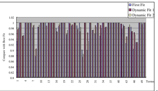
(18) Table 2: Parameter setting. The inter arrival time of new Logical Channel are used to determinate the numbers of TTI M. in one simulation term. Moreover, in our evaluation function E (k ) = ∑ Wi ∗ D[k ][i ] , we will i =1. adopt Wi = 9 – P[i] for each logical channel i in our experimental simulation because of the higher priority, we have the lower P[i] value. 4.2 Simulation Results The simulation results of earning-rate and total-rate are as follows. From the figure 10 and 11, we can found the dynamic fit 2 earn more rewards than first fit in most situation and almost the same with best fit. Besides, the total rate of dynamic fit 2 is fewer than first fit and best fit. First Fit Dynamic Fit 1 Dynamic Fit 2. 1.02 1. 0.96 0.94 0.92 0.9 0.88 0.86 0.84 0.82 49. 46. 43. 40. 37. 34. 31. 28. 25. 22. 19. 16. 13. 10. 7. 4. 0.8 1. Compare with Best Fit. 0.98. Terms Figure 10: the. comparison of earning-rate between three methods.

(19) First Fit. 1.8. Dynamic Fit 1. 1.6. Dynamic Fit 2. Compare with Best Fit. 1.4 1.2 1 0.8 0.6 0.4 0.2. 49. 47. 45. 43. 41. 39. 37. 35. 33. 31. 29. 27. 25. 23. 21. 19. 17. 15. 13. 9. 11. 7. 5. 3. 1. 0 Terms Figure 11: the comparison of total-rate between three methods. 5. Conclusions Because of the rapid growth of wireless services, an increasing number of users transmit data through air interface by sharing the limited bandwidth. However, that will incur a lack of the applicable bandwidth. Therefore, how to offer the appropriate bandwidth size on demand for each mobile equipment has become an important part of the radio resource control. In this paper, we provide three TFC selection methods. Theses methods consist of two phases, assignment step and selection step. The former performs the mapping between logical channels and transport channels and decide how much data for each logical channel can be transmitted in the next TTI for each TFC if we choose it to transfer while the latter is used to select an appropriate TFC from the TFCS based upon the results from the assignment step. To compare the effectiveness of these TFC selection methods, we also conducted some experiments. Our results confirm that even if the best_fit often do the best effectiveness, we still prefer to adopt the dynamic_fit assignment algorithm. On one hand it can save more execution time, and on the other hand the selected TFC through dynamic_fit assignment algorithm often has lower bit rate so as to economize total transmitted power and decrease the possible interference.. 6. References [1] [2] [3] [4]. 3GPP 3GPP 3GPP 3GPP. TS TS TS TS. 25.302: 25.321: 25.331: 25.303:. "Services provided by the physical layer". "MAC protocol specification" "Radio Resource Control (RRC); protocol specification" "Interlayer Procedures in Connected Mode"..

(20)