下鏈LTE-A蜂巢式系統中協調式多點傳輸方法之研究

國 立 交 通 大 學

電信工程研究所

碩 士 論 文

下鏈 LTE-A 蜂巢式系統中協調式多點傳輸方法

之研究

A Study on Coordinated Multi-Point Transmission

(CoMP) Scheme for the Downlink LTE-A Cellular

System

研 究 生: 楊為守

指導教授: 黃家齊 博士

下鏈 LTE-A 蜂巢式系統中協調式多點傳輸方法之研究

A Study on Coordinated Multi-Point Transmission (CoMP)

Scheme for the Downlink LTE-A Cellular System

研 究 生：楊為守

Student: Wei-Shou Yang

指導教授：黃家齊 博士

Advisor: Dr. Chia-Chi Huang

國 立 交 通 大 學

電信工程研究所

碩 士 論 文

A Thesis

Submitted to Institute of Communication Engineering

College of Electrical and Computer Engineering

National Chiao Tung University

in Partial Fulfillment of the Requirements

for the Degree of

Master of Science

in

Communication Engineering

July 2012

Hsinchu, Taiwan, Republic of China

下鏈 LTE-A 蜂巢式系統中協調式多點傳輸方法之研究

研究生：楊為守

指導教授：黃家齊 博士

國立交通大學電信工程研究所 碩士班

摘

要

協調式多點傳輸 (Coordinated Multi-Point Transmission，CoMP) 是一種有效降低基 地台間干擾的方法。其主要概念是挑選數個基地台彼此合作以消除干擾，這衍生出一個 問題：哪些基地台該合作並形成一個協調式多點傳輸叢集 (CoMP Cluster)？針對下鏈傳 輸，我們提出一個動態建立叢集的方法。為了降低複雜度，我們使用一種基於區塊對 角化 (Block Diagonalization) 的線性前置編碼器。模擬結果顯示出此動態方法優於另一 靜態方法。接下來，我們提出一最佳的功率分配方式，使得總傳輸功率最低並同時滿 足誤碼率 (Bit Error Rate)、資料傳輸率與天線傳輸功率限制。我們使用 Lagrange 對偶分 解 (Dual Decomposition) 來解決此非凸 (Non-Convex) 的最佳化問題。和一固定的功率分 配方式比較後，模擬結果顯示此最佳化方法能提供較佳的效能，此外，各天線上的傳 輸功率也較少超出其限制。最後，我們提出了一個降低峰均值功率比 (Peak-to-Average Power Ratio，PAPR) 的方法，其使用疊代的方式來改變星座點以降低 PAPR。模擬結果

A Study on Coordinated Multi-Point Transmission (CoMP)

Scheme for the Downlink LTE-A Cellular System

Student: Wei-Shou Yang

Advisor: Dr. Chia-Chi Huang

Institute of Communication Engineering

National Chiao Tung University

ABSTRACT

Coordinated multi-point transmission (CoMP) is a promising way to suppress inter-base

station (BS) interference. The main idea of CoMP is to select several BSs which could

coop-erate together to mitigate interference, which raises an intrinsic problem of which BSs should

form a CoMP cluster. We propose a dynamic clustering method for downlink transmission,

which forms CoMP clusters adaptively. To reduce the complexity, a linear precoder based on

block diagonalization (BD) is used throughout this thesis. Simulation results show that our

dynamic scheme outperforms another static method. Next, we design an optimal power

allo-cation method that minimizes the total transmit power while satisfying bit error rate (BER),

user rate requirement and per-antenna power constraints. Lagrange dual decomposition is used

to solve this non-convex optimization problem. The numerical results reveal the great

perfor-mance gain against fixed power allocation, and the transmit power on each antenna seldom

exceeds the power limit. Finally, we propose a peak-to-average power ratio (PAPR) reduction

method, which reduces signal peak by altering signal constellations. The simulation results

誌 謝

TABLE OF CONTENTS

中文摘要 i

ABSTRACT ii

誌謝 iii

LIST OF FIGURES vii

LIST OF TABLES viii

CHAPTER 1 INTRODUCTION 1

1.1 CoMP Concept . . . 2

1.2 Resource Allocation . . . 4

1.3 PAPR Reduction . . . 5

1.4 Organization of this thesis . . . 6

CHAPTER 2 CLUSTERING TECHNIQUES FOR COMP 8 2.1 System Model and Transmission Schemes . . . 8

2.1.1 Single Cell Processing . . . 9

2.1.2 Base Station Cooperation . . . 12

2.2 Clustering Algorithms . . . 14

2.2.1 Static Clustering . . . 14

2.2.2 Dynamic Clustering . . . 16

2.3 Simulation Results . . . 19

CHAPTER 3 ADAPTIVE RESOURCE ALLOCATION 27 3.1 System Model and Transmission Schemes . . . 27

3.2 Problem Formulation . . . 28

3.3 Low Complexity Solution for Power Minimization . . . 30

3.3.1 Optimization Based on Dual Decomposition . . . 30

3.3.2 Convergence Behavior Control . . . 35

CHAPTER 4 PAPR REDUCTION FOR MU-MIMO SYSTEMS 44

4.1 System Model and Transmission Schemes . . . 44

4.2 Suboptimal Power Minimization Algorithm . . . 45

4.3 Multiuser Active Constellation Extension Method . . . 46

4.3.1 PAPR Definition and ACE Concept . . . 46

4.3.2 Problem Formulation . . . 48

4.3.3 An Efficient Algorithm for ACE . . . 50

4.3.4 Modifications of ACE . . . 54

4.4 Simulation Results . . . 55

CHAPTER 5 CONCLUSION 61 APPENDIX A DERIVATIONS FOR CHAPTER 3 63 A.1 Derivation of Competitive Water Filling Solution . . . 63

A.2 Derivation of Supergradient . . . 65

LIST OF FIGURES

Figure Page

1.1 Illustration for CoMP-JT mode. The solid arrows stand for the signal links. . . 2

1.2 Illustration for CoMP-CB mode. The solid arrows stand for the signal links and the dashed ones are the interfering links. . . 3

2.1 A clustering example with B = 2 and Nb = 4. . . 9

2.2 Proposed static clustering table when cluster size B = 3. . . . 16

2.3 A snapshot of the dynamic clustering. . . 18

2.4 Average rate versus the edge-SNR. . . 20

2.5 The average rate versus different pilot SINR threshold. . . 22

2.6 The CDF of the CoMP requesting users. . . 24

2.7 The CDF of the CoMP included users. . . 24

2.8 The CDF of the last five percent users. . . 25

2.9 The average rate versus different CoMP cluster size. . . 26

2.10 The CDF of the CoMP requesting users using weighted sum utility versus different CoMP cluster size. . . 26

3.1 Block diagram for downlink multi-user MIMO-OFDM. . . 27

3.2 Flowchart of our resource allocation algorithm. . . 37

3.3 Illustration for three-sectorized CoMP. . . 38

3.4 Edge-SNR versus different target rate. . . 40

3.5 Edge-SNR versus different number of antennas. . . 40

3.6 User rate convergence behavior. . . 42

3.7 Sum-power convergence behavior. . . 42

3.8 Normalized transmit power on antenna 1 over 100 channel realizations when pcon_a ∼= 8.019 W. . . . 43

3.9 Normalized transmit power on antenna 1 over 100 channel realizations when pcon a ∼= 1.271 W. . . . 43

4.2 Illustration for ACE with 16-QAM modulation. . . 48

4.3 Illustration of block-IDFT. . . 49

4.4 The SNR versus different rate requirements. . . 56

4.5 A snapshot of the data symbols with QPSK modulation after ACE. . . 56

4.6 A snapshot of the data symbols with 16-QAM modulation after ACE. . . 57

4.7 The CCDF of the PAPR after ACE. . . 58

4.8 The CCDF of the PAPR after ACE with different oversampling factors. . . 58

4.9 The CCDF of the PAPR after ACE with different PAPR targets. . . 59

LIST OF TABLES

Table Page

2.1 The CoMP request ratio and the actual CoMP included ratio against different pilot SINR threshold. . . 21

CHAPTER 1

INTRODUCTION

With the demand of high data rate in the future wireless communication systems,

multiple-input multiple-output (MIMO) techniques have been proposed to improve the system

through-put. Besides, in a cellular network, the frequency band can be reused in a one cell fashion to

maximize the spectral efficiency. However, one cell frequency reuse limits the performance of

MIMO systems due to severe other-cell interference (OCI) [1]. Although the receiver can

elim-inate the interference by applying techniques like successive interference cancellation (SIC),

but in the downlink, this burdens the user equipment (UE) with high computational

complex-ity. Recently, a promising way called CoMP has been proposed by the long-term evolution

advanced (LTE-A) to suppress OCI. The idea of CoMP is to gather a group of BSs which share

channel state information (CSI) and/or user data via high speed backhaul. In this way, the BSs

can cooperate to lower the interference. On the other hand, since the channel varies with the

user location, we can allocate power in different domains like frequency and space according to

their channel quality. LTE-A prescribes orthogonal frequency division multiplexing (OFDM)

for downlink transmission, such a multi-tone system suffers from high PAPR, which reduces

the transmit power efficiency. In this thesis, we discuss the CoMP, power allocation and PAPR

reduction issues, and some algorithms suitable for BS coordination scenario are proposed. It

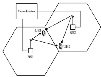
Figure 1.1: Illustration for CoMP-JT mode. The solid arrows stand for the signal links.

1.1

CoMP Concept

In LTE-A downlink, there are two classes of CoMP schemes named joint transmission (JT)

and coordinated beamforming (CB). One can distinguish these two modes by the type of

infor-mation sharing. The former requires both CSI and data exchange and the latter needs only CSI

exchange.

The concept of CoMP-JT can be illustrated using Figure 1.1. Conceptually, the cellular

network which deploys CoMP-JT is equivalent to multi-user MIMO (MU-MIMO) with some

distinctions that the transmit antennas now belong to distributed BSs and the channels to

differ-ent users experience independdiffer-ent pathloss and shadowing. Joint transmission means the signal

intended for any user is jointly pre-processed and transmitted from all the BSs. Therefore, the

interfering links (a link is the channel from a BS to a user) are transformed into useful links.

The drawback of this mode is that the data for every user and the CSI of all the links need to be

shared among the BSs, which increases the backhaul overhead.

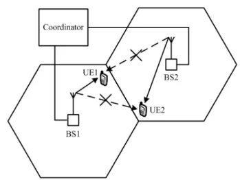
In the case of CoMP-CB (see Figure 1.2), as conventional single cell scheme, each BS

Figure 1.2: Illustration for CoMP-CB mode. The solid arrows stand for the signal links and the

dashed ones are the interfering links.

the other cell by acquiring the CSI of the interfering links. In this mode, there is no data

shar-ing, which reduces the backhaul traffic. However, the design target is to eliminate the generated

interference but not to make use of it, which leads limited performance gain compared to

CoMP-JT. In both cases, the users need to feedback the CSI from all the links including the interfering

ones. In time division duplex (TDD) mode, the job of channel estimation can be placed in either

BS or user side, while in frequency division duplex (FDD) mode, user has to estimate the CSI

and feedback through uplink channels.

Plentiful research works on CoMP-JT can be found in the recent years [2]-[6]. [2] gives

an overview including the currently known techniques for JT (also a part of

CoMP-CB), practical issues related to system complexity and main challenges for future CoMP design.

A straightforward way to implement CoMP-JT is to build a central coordinator (CC) which

collects all the CSI and then computes the precoding weights for all the users. The performance

analysis to this way, using nonlinear (dirty paper coding, DPC) and linear (zero-forcing, ZF and

minimum min square error, MMSE) precoding, was studied in [3] and [4], respectively. Such a

to overcome this problem is dividing the BSs into several clusters [5], [6].

As for CoMP-CB, [7] proposed a beamforming algorithm which aims to find the interfering

users with similar channels. Another way to suppress interference using distributed resource

allocation is discussed in [8]. In this thesis, we mainly focus on CoMP-JT.

In order to reduce the overhead, there are only a limited number of BSs can be included in

a CoMP cluster. This leads to the question which BSs should form the clusters to maximize the

system performance at manageable complexity. Static [9] and dynamic [10] clustering are two

types of forming CoMP clusters. Static clustering can be performed in advance based on field

measurements or geographical relations. Whereas dynamic clustering exploits CSI and changes

the cluster groups over time. Algorithms for these two types can be found in Chapter 2.

1.2

Resource Allocation

After the BSs in the cellular network are grouped into several CoMP clusters, there are more

jobs we can do in each cluster to improve the system performance. OFDM is chosen to be

the modulation scheme for the downlink LTE-A, one advantage of the multicarrier system is

that the power and rate can be allocated over different tones according to their variety if the

transmitter has the CSI. In general, there are two objectives of resource allocation: the sum-rate

maximization and power minimization [11], [12]. We pay our attention on the latter in this thesis

for power saving.

Traditionally, resource allocation problems are formulated under sum-power constraint on

the transmit antennas. However, per-antenna power constraint would be more realistic since

each antenna has independent power amplifier. Besides, for avoiding inter-user interference,

many systems apply orthogonal frequency division multiple access (OFDMA) technique which

im-proved by separating the users in the spatial domain when the transmitter equips multiple

an-tennas [13], in this way, multiple users can share the same subcarrier. As for the user terminals,

different users may have individual quality of service (QoS) requirements such as minimal data

rate and acceptable bit error rate (BER).

In Chapter 3, the power minimization problem under user rate and BER constraints as in

[12] is considered. To make this problem more general, we add additional per-antenna power

constraint and extend the system to a multi-cell scenario. The problem is non-convex since it

aims to find the optimal set among different subcarrier and user combinations, and the

com-plexity increases exponentially with the number of subcarriers and users. Therefore, efficient

solutions must be found to make the complexity feasible. Although the original problem is not

convex, it can be transformed to another problem based on Lagrange dual decomposition [12].

The transformed problem is always concave regardless of the convexity of the original problem.

In this way, conventional convex optimization techniques can be applied to solve this problem

efficiently.

1.3

PAPR Reduction

Although the average transmit power can be minimized via the techniques introduced in

Chapter 3, however, the power consumption of the power amplifier (PA) is dominated by the

peak power rather than the average power. One of the main drawbacks of OFDM is the large

PAPR, which makes the efficiency of the PA very poor (the definition of PAPR is left in section

4.3.1. In order to transmit a signal with wide power rang, an expensive PA is needed. For

im-proving the power efficiency, several classes of PAPR reduction techniques have been proposed

[14]-[16].

re-serves some unused subcarriers and inserts signals to reduce the PAPR. This method causes

no distortion to the data-carrying subcarriers due to the orthogonality of subcarriers. However,

there exists a tradeoff between the PAPR reduction performance and the number of the reserved

subcarriers. Reserving more subcarriers yields better performance, but sacrifices the available

bandwidth for transmitting information data.

Another class called active constellation extension (ACE) tries to reduce PAPR by altering

the constellation of the data [15], [16]. Without reserving any subcarrier, this scheme maps the

original constellation to a constrained space which produces lower PAPR.

In Chapter 4, we first propose a suboptimal power allocation algorithm to reduce the

av-erage transmit power. As stated above, the power consumption depends mainly on the peak

power. Hence we introduce a PAPR reduction scheme which combines tone reservation and

constellation extension. This scheme is based on the idea of [15]. Additionally, we made some

modifications so that it is suitable for CoMP-JT systems. As a note, this approach is designed

for the signal which employs quadrature amplitude modulation (QAM).

1.4

Organization of this thesis

The rest of this thesis is organized as follows. In Chapter 2, we start with the CoMP clustering

concept. How does a cellular network implement CoMP and which BSs should form a CoMP

cluster will be illustrated. In Chapter 3, assuming all the CoMP clusters have been planned, we

design an optimal power allocation method for each cluster. For power saving, the objective is

to minimize the total transmit power. Chapter 4 deals with the problem of PAPR. A practical

PAPR reduction algorithm suitable for the CoMP system is proposed. Finally, Chapter 5 gives

the conclusion of this thesis. It should be noted that Chapter 2 - 4 have their own system models

Throughout this thesis, we adopt some notations: Matrix and vectors are denoted by

up-percase and lower case boldface letters; IN is the N × N identity matrix; A [i, j] indicates the

element in the row i and column j of the matrix A;∥ · ∥2

F and∥ · ∥2∞are the Frobenius norm

and infinity norm; (·)∗, (·)T and (·)H represent the conjugate, transpose and conjugate transpose operators.

CHAPTER 2

CLUSTERING TECHNIQUES FOR COMP

2.1

System Model and Transmission Schemes

Consider a downlink cellular network consists of Nb BSs with Nt antennas each and Kb

active users in the bth _{cell with N}

r antennas each. All the BSs operate on the same carrier

frequency so they will cause interference to each other. Assume that the BSs in the network

are divided into several clusters, each contains B BSs, where B ≤ Nb (see Figure 2.1). The

clusters are all non-overlapping groups. In other words, if one BS has been involved in a cluster,

it cannot join the others. LetG be one of the set of the selected BSs in a cluster. The received signal of the kth _{user in the b}th_{cell of the set}G can be written as

yG_k,b = Hb_k,bxk,b+ ∑ i̸=k,i↔b Hb_k,bxi,b+ ∑ b∈G,b̸=b ∑ j↔b Hb_k,bx_j,b+∑ eb/∈G ∑ l↔eb Heb_k,bx_l,eb+ nk,b, (2.1)

where Hb_k,bis the Nr× NtMIMO channel from the BS b to the user k served by the BS b, xk,bis

the Nt×1 transmitted signal and nk,bis the corresponding Nr×1 received noise vector, in which

each element is a zero-mean complex Gaussian random variable with variance N0. The first term

of (2.1) is the desired signal, the second is the inter-user interference (IUI) in the bth_{cell where}

i↔ b means the user i is served by the BS b, the third is the intra-cluster interference (ICI) from the BSs in the clusterG except the BS b, and the last term is the outer-cluster interference (OCI) from the BSs outside the clusterG.

Figure 2.1: A clustering example with B = 2 and Nb = 4.

2.1.1

Single Cell Processing

In this scenario, each BS serves its users without coordinating with the other BSs, i.e., B = 1.

Assume the bth_{BS is considered. The transmit precoding matrices for the user k in the BS b are}

designed in the following two cases respectively.

Case 1) Eigenmode Precoding for Kb = 1

When there is only one user per BS, the received signal of the user k in the cell b can

be written as y_k,b = Hb_k,bxk,b+ ∑ b̸=b ∑ i↔b Hb_k,bx_i,b+ nk,b. (2.2)

Note that the index for cluster is ignored here since there is no clustering concept when

B = 1. When each BS has only the CSI of its served user, the precoding matrix can be designed by performing singular value decomposition (SVD) on Hb_k,b:

Hb_k,b = Ub_k,bS_k,bb (Vb_k,b)H, (2.3) where Sb_k,b ∈ CNr×Nt _{is the matrix which contains the singular values, U}b

k,b ∈ CNr×Nr

and Vb_k,b∈ CNt×Nt _{collects the left and right singular vectors, respectively. Let P}b k,bbe

the power allocation matrix for the user k in the BS b. Here we assume a simple equal

power allocation, that is

Pb_k,b=(√pcon_/N

r

)

where pconis the sum power constraint per BS. The precoding matrix can be chosen as

Fb_k,b= Vb_k,b (2.5) and the receive equalization matrix is

Qb_k,b=(Ub_k,b)H. (2.6) Having the precoding matrix, the pre-processing can be done as

xb_k,b = Fb_k,bPb_k,bdb_k,b, (2.7) where db_k,b ∈ CNr×1 _{represents the information data. After receive equalization, the}

signal becomes rk,b = Qbk,byk,b = Qb_k,b  Hb k,bxk,b+ ∑ b̸=b ∑ i↔b Hb_k,bx_i,b+ nk,b   =(Ub_k,b)HUb_k,bSb_k,b(V_k,bb )HVb_k,bPb_k,bdb_k,b+ Qb_k,b∑ b̸=b ∑ i↔b Hb_k,bx_i,b+ Qb_k,bnk,b = Sb_k,bPb_k,bdb_k,b+∑ b̸=b ib_k,b+enk,b, (2.8) where ib_k,b = ∑ i↔b

Qb_k,bHb_k,bx_i,b is the equivalent interference from BS b. Therefore the spatial streams can be extracted as

rk,b,l = sbk,b,l √ pb k,b,ld b k,b,l+ i b k,b,l+enk,b,l, 1≤ l ≤ Nr, (2.9)

where db_k,b,lis the lthelement of db_k,b, sb_k,b,land pb_k,b,lare the corresponding singular value and the power loading weight, respectively, ib

k,b,l is the interference on the lth stream

andenk,b,l is the complex Gaussian noise with variance N0. As a result, the Nr × Nt

MIMO channel Hb_k,b is decoupled into Nr parallel single-input single-output (SISO)

signal-to-interference plus noise ratio (SINR) of the lthstream for the user k in the BS b is SIN Reigen_k,b,l = ( sb k,b,l )2 pb k,b,l E [ ∑ b̸=b ib k,b,l ( ib k,b,l )_∗] + N0 (2.10)

and the capacity is

C_k,beigen =

Nr

∑

l=1

log₂(1 + SIN Reigen_k,b,l ). (2.11) Case 2) Block Diagonalization (BD) [13] for Kb > 1

In this case, the interference seen by the user k in the BS b can come from the other

users in the same BS and those in the other BSs. The received signal can be written as

y_k,b = Hb_k,bxk,b+ ∑ i̸=k,i↔b Hb_k,bxi,b+ ∑ b̸=b ∑ j↔b Hb_k,bx_j,b+ nk,b. (2.12)

Having only the CSI of the users in its scope, each BS can apply BD to eliminate the

IUI, i.e., the second term of (2.12). There is a restriction on BD, which is Nt≥ KbNr,

that is, the number of the transmit antennas must be larger than or equal to the sum of

the number of the receive antennas. We introduce the procedure of designing the BD

precoder below.

For simplicity, the index for BS is ignored here. The composite channel of all the users

in the cluster can be written as H =[HT₁, . . . , HT_K]T ∈ CKNr×Nt_{. Then we collect the}

interfering channels to the user k and apply SVD as

[ HT₁, . . . , HT_k−1, H_k+1T , . . . , HT_K]T = UkSk [ VkVk ]H , (2.13)

where Vk ∈ CNt×(Nt−(K−1)Nr)is the matrix which contains the right singular vectors

that correspond to the zero singular values and therefore is the null space. The

equiva-lent channel to the user k after orthogonalization is given by

e

Apply SVD again on eHkand get

e

Hk= eUkeSkeVk. (2.15)

Similarly, we can use eigenmode precoder to decompose the equivalent MIMO channel

e

Hk. The transmit precoding matrix can be designed as

Fk = VkeVk (2.16)

and the receive equalization matrix is

Q_k= eUH_k. (2.17) Hence, the users in the BD deployed BS will not observe interference from each other

because their channels are mutually orthogonal, although the interference from the other

BSs still remains. Since there are K users now, the power allocated to each user should

be divided by K. Thus, the power allocation matrix should be

Pk = (√ pcon_/KN r ) INr. (2.18)

Since the inter-user interference is eliminated, the capacity for the user k can be

repre-sented in the same form as 2.11, the difference is that each BS now applies BD but not

eigenmode precoding.

2.1.2

Base Station Cooperation

In this section, we show where the BD algorithm should be modified when it is applied to a

multi-cell scenario. Assume a CoMP clustering algorithm is applied and some CoMP clusters

are formed. In JT mode, all the users' information data and channels are shared among the BSs in

the same cluster. Therefore, the grouped BSs can be seen as a huge BS with additional antennas.

scope. The multi-cell BD can be done in a way similar to the Case 2 of single cell processing with

some little differences that the transmit antenna Ntbecomes BNtand the sum power constraint

pcon _{changes to Bp}con_{. Like single cell BD, the channels of all the users in the same cluster will}

become orthogonal to each other after multi-cell BD. Therefore, the interference only comes

from the BSs outside the cluster, and the received signal of the user k in the BS b of the cluster

G can be written as yG_k,b = HG_k,bxG_k,b+∑ b /∈G ∑ i↔b Hb_k,bx_i,b+ nG_k,b, (2.19) where HG_k,bis the Nr×BNtmulti-cell MIMO channel and xGk,bis the BNt×1 transmitted signal.

The joint BD precoding matrix is

FG_k,b = VG_k,beVG_k,b, (2.20) where VG_k,bis the null space of the other users inG except the user k and eVG_k,bis the matrix which collects the first Nrright singular vectors of the projected channel eHGk,b = HGk,bV

G

k,b. The jointly

pre-processed signal can be represented as

xG_k,b= FG_k,bPG_k,bdG_k,b, (2.21) where the power allocation matrix is

PG_k,b=  √Bpcon_/∑ b∈G KbNr   INr, (2.22)

(assume every BS has the same transmit power constraint pcon_{) and d}G

k,bis the information data.

If the user k chooses the equalization matrix to be

QG_k,b= ( eUG k,b )H , (2.23)

where eUG_k,bcontains the left singular vectors of the projected channel eHG_k,b. The equalized signal at the receiver side can be derived following the similar steps of (2.8) and given by

rG_k,b = QG_k,b  HG k,bxGk,b+ ∑ b /∈G ∑ i↔b Hb_k,bx_i,b+ nG_k,b   = QG_k,bHG_k,bVG_k,beVG_k,bPG_k,bdG_k,b+∑ b /∈G ∑ i↔b QG_k,bHb_k,bx_i,b+ QG_k,bnG_k,b = ( eUG k,b )H eUG k,beSGk,b ( eVG k,b )H eVG k,bPGk,bdGk,b+ ∑ b /∈G ib_k,b+enG_k,b = eSG_k,bPG_k,bdG_k,b+∑ b /∈G ib_k,b+enG_k,b. (2.24) Being similar to (2.9), the multi-cell MIMO channel is decoupled and the lth_{spatial stream is}

r_k,b,lG = sG_k,b,l √

pG_k,b,ldG_k,b,l+ ib_k,b,l+enG_k,b,l, 1≤ l ≤ Nr. (2.25)

The SINR of the lth_{stream for the user k in the BS b of the clusterG is}

SIN RCoMP_k,b,l = ( sG_k,b,l)2pG_k,b,l E [ ∑ b /∈G ib k,b,l ( ib k,b,l )_∗] + N0 (2.26)

and the capacity is

C_k,bCoMP =

Nr

∑

l=1

log₂(1 + SIN RCoM P_k,b,l ). (2.27) In BS cooperation scenario, the signal from different BSs will experience different delay.

There-fore, synchronization is an important topic. Nevertheless, to simplify our system, we assume

the synchronization is always perfect.

2.2

Clustering Algorithms

2.2.1

Static Clustering

Static clustering is a feasible way to form the clusters in the cellular network. It can be

determined, it will not change over time. The advantage of this clustering type is that routing

CSI and user data to a central coordinator (CC) is unnecessary. Instead, it requires a distributed

coordinator (DC) per cluster which controls the BSs. The cooperation only takes place in each

cluster and different clusters do not communicate with each other, which reduces the overheads.

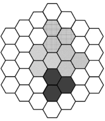
Here we propose a static clustering algorithm as follow. In each cell, we assume there is only

one scheduled user, so the index for user can be ignored and the new notation Hb_bstands for the channel from the BS b to its user.

Algorithm Static Clustering Algorithm.

1: Specify the CoMP cluster size B;

2: Each user measures channel gains and calculates his pilot SINR by

SIN Rpilot_b = Hb_b 2/   ∑ b̸=b,b∈Ib Hb b 2 + N0   , ∀b, (2.28) whereIbis set of the six first tier interfering BSs around BS b, i.e., only the pilots from the

neighboring BSs are regarded as the valid interference. If SIN Rpilot_b < γ, where γ is the threshold, the user requests CoMP service to the BS b through uplink. Then BS b sends the

request to its DC;

3: DC finds the remaining B− 1 BSs which should cooperate with the BS b based on the pre-defined clustering table (see Figure 2.2 for the case of B = 3), and makes them to form a

cluster;

4: Go back to step3 until all the CoMP needed users are satisfied;

The clusters are formed by neighboring BSs here. Since in average, they cause stronger

in-terference compared with those farther BSs. Although static clustering reduces the inter-cluster

communication overhead, it inherits the fairness problem from single cell scenario that the users

Figure 2.2: Proposed static clustering table when cluster size B = 3.

2.2.2

Dynamic Clustering

Static clustering has very limited performance gain since the variation of the channel

con-dition is not fully exploited. As mentioned in the previous section, we select the neighboring

BSs to form static clusters. Since on average, they are the ones which cause strong

interfer-ence. Nevertheless, due to the effect of shadowing, a user might experience a better channel to

a farther BS, in other words, interference does not always come from near BSs. Therefore, it

is not flexible to form fixed clusters by grouping BSs which are close to each other. Besides,

users at the edge of the static cluster experience much more interference from the neighboring

clusters than the ones located around the center of the cluster, which causes fairness problem. In

order to overcome the aforementioned problems, the idea of dynamic clustering has been

intro-duced. Geographical relation is not the main concern anymore. Instead, we try to group the BSs

which cause the strictest interference before any cooperation. The proposed greedy algorithm

Algorithm Dynamic Clustering Algorithm.

1: Specify the CoMP cluster size B;

2: Each user calculates his SIN Rpilot_b as defined in (2.28). If SIN Rpilot_b < γ, the user sends CoMP request to the serving BS b;

3: The CC collects all the requests and chooses a CoMP needed user who has not been chosen

so far uniformly;

4: Find the remaining B− 1 BSs which maximize the utility function J(C₁CoMP, . . . , C_BCoMP) with the user chosen in step 3, where CCoMP

b is the capacity given by (2.27). We let only the

first tier BSs around the selected user to be the candidates, i.e., b∈ Ib. If the available BSs

is less than B− 1, the user cannot acquire CoMP service at this time slot, then CC drops this user and picks another one uniformly;

5: Go back to step 3 until all the CoMP needed users find their partners;

We provide three choices of the utility function in this dynamic algorithm:

• Sum-rate (SR) utility: J1 = 1 B B ∑ b=1 C_bCoMP (2.29)

• Proportional fair (PF) utility:

J2 = ( _B ∏ b=1 C_bCoMP )1/B (2.30)

• Weighted sum (WS) utility:

J3 =

B

∑

b=1

wbCbCoMP (2.31)

The purpose of the weight is to find the users who really need CoMP, i.e., the users with low

SINR. So the weight is set to the reciprocal of the SINR, which is

where qb = log2 ( 1 + SIN Rpilot_b ) (2.33)

is the transformed SINR which approximates capacity and

c = 1 B ∑ b=1 q−1_b (2.34)

is a normalization factor such that

B

∑

b=1

wb = 1. Note that SIN Rpilot_b is the SINR experienced by

the users before CoMP. The user with larger SIN Rpilot_b will get lower weight, since the perfor-mance gain is little when apply CoMP to the users with high SINR.

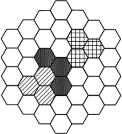
Figure 2.3 shows a snapshot of the dynamic clustering result. No matter which utility

func-tion is chosen, the CoMP clusters can be formed adaptively according to the change of channel

conditions. Hence there are no constant cluster edges and therefore no users will suffer from

more interference. However, there must exits a CC to run the dynamic clustering algorithm.

Besides, the overhead of routing the CSI and user data is higher than the static scheme.

Since the available BSs for selection are reducing through the dynamic algorithm, it benefits

the user that is chosen earlier in Step 3. To circumvent this fairness issue, we have to choose the

user uniformly. Therefore, on average, everyone obtains close performance gain.

2.3

Simulation Results

We consider a downlink network consists of thirty-seven cells overall (Nb = 37), i.e., the

first three tiers of cells, each cell has one BS at its center. Every BS has two omnidirectional

antennas (Nt = 2) and each user has two antennas (Nr= 2). The cell radius is set to 1 Km. The

MIMO channel from the BS b to the user k served by the BS b is

Hb_k,b = Rb_k,b/ √ β ( db k,b )α sb k,b, (2.35)

where Rb_k,bis the Nr× NtRayleigh fading channel, in which the elements are all i.i.d. complex

Gaussian random variables, sb

k,b is log-normal distributed with 8 dB standard deviation which

models the shadowing effect and db_k,bis the corresponding distance in Km. For the pathloss, the 3GPP LTE pathloss model [10] is used, where β = 1014.81 _{and α = 3.76. The noise power}

spectral density is -174 dBm/Hz. Suppose that all of the BSs transmit on the same subcarrier

with 15 KHz subcarrier spacing, so the noise power is N0 ∼= −162.2391 dBW. One user is

generated uniformly in each cell (Kb = 1, ∀b) to simulate the round-robin scheduling, and we

assume the user has not been handed off to another cell, i.e., the user generated in the cell b is

served by the BS b, although the strongest signal may come from another BS. The cluster size

B is fixed to three unless otherwise stated. We only observe the performance of the user in the central cell in the network, whereas all of the users in the central cell and its first tier BSs (total

seven users) are allowed to request CoMP service. For our observed user in the central cell, only

the signals from the six first tier BSs are treated as interference. The six BSs could be CoMP or

non-CoMP BSs, which depends on the result of our clustering algorithm. If it is a CoMP BS,

it deploys multi-cell BD (see section 2.1.2) with its partners. Otherwise, it applies single cell

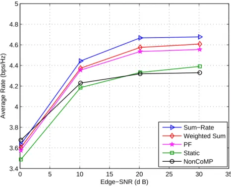
0 5 10 15 20 25 30 35 3.4 3.6 3.8 4 4.2 4.4 4.6 4.8 5 Edge−SNR (d B) Average Rate (bps/Hz) Sum−Rate Weighted Sum PF Static NonCoMP

Figure 2.4: Average rate versus the edge-SNR.

Figure 2.4 shows the average rate as a function of the edge-SNR when the pilot SINR

thresh-old γ =−8.3 dB. The edge-SNR is defined as the SNR measured by the user located at cell-edge without shadowing and interference, which is given by

SN Redge(dB) = pcon(dBW)− 10log₁₀(β)− 10αlog₁₀(rcell)− N0(dBW) , (2.36)

where rcellis the cell radius. In (2.36), we count the transmit power from only one BS, but each

user receives multiple signal from all the BSs in the same CoMP cluster in our simulation. We

can see that all the clustering schemes outperform the non-CoMP one when SN Redge _{> 20 dB}

since the interference is reduced. The three dynamic approaches provide better average rate gain

against the static clustering because they exploit the instantaneous CSI. Due to the target of the

utility function, using sum-rate utility gets the best average rate and weighted sum is better than

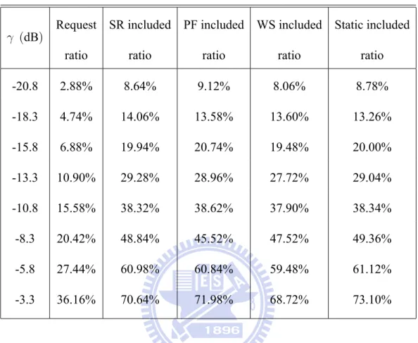
Table 2.1: The CoMP request ratio and the actual CoMP included ratio against different pilot SINR threshold. γ (dB) Request ratio SR included ratio PF included ratio WS included ratio Static included ratio -20.8 2.88% 8.64% 9.12% 8.06% 8.78% -18.3 4.74% 14.06% 13.58% 13.60% 13.26% -15.8 6.88% 19.94% 20.74% 19.48% 20.00% -13.3 10.90% 29.28% 28.96% 27.72% 29.04% -10.8 15.58% 38.32% 38.62% 37.90% 38.34% -8.3 20.42% 48.84% 45.52% 47.52% 49.36% -5.8 27.44% 60.98% 60.84% 59.48% 61.12% -3.3 36.16% 70.64% 71.98% 68.72% 73.10%

Table 2.1 gives the probability of the CoMP requesting users and the actual CoMP included

users with different pilot SINR threshold when SN Redge ∼_{= 30 dB. In both of the static and}

dynamic algorithms, there are two types of users named the CoMP requesting users and the

CoMP included users. The CoMP requesting user is the one whose pilot SINR is lower than the

threshold, in other words, is the user who sends CoMP request. The CoMP included users are

the CoMP requesting user plus the B− 1 users who are forced to get CoMP service (see the clustering algorithm in either section 2.2.1 or 2.2.2. For instance, if B = 3 and the user in the

BS 1 sends a CoMP request. The coordinator makes the users in the BS 2 and 3 to be the CoMP

partners of the user in the BS 1. Then the user served by the BS 1 is called the CoMP requesting

user and all of them are called CoMP included users. This table tells us the percentage of these

static CoMP included users is higher than the three dynamic ones when the threshold is high.

Because when the threshold is getting larger, more and more users request CoMP. As a result,

some CoMP requesting users in the dynamic clustering algorithm cannot find sufficient BSs to

form a cluster.

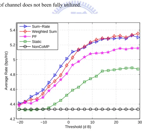
Figure 2.5 plots the average rate versus different pilot SINR threshold when SN Redge ∼₌

30 dB, which corresponds to pcon _{= 16 dBW. As stated in Table 2.1, with the increasing of the}

threshold, more users can request CoMP and therefore the average rate is getting better with the

price of higher network overhead. The average rates saturate when the threshold is high enough

(about 15 dB above), since almost 100 % users are included in CoMP areas now. The static

scheme obtains relatively low performance gain compared to the three dynamic ones because

the variety of channel does not been fully utilized.

−20 −10 0 10 20 30 4.2 4.4 4.6 4.8 5 5.2 5.4 Threshold (d B) Average Rate (bps/Hz) Sum−Rate Weighted Sum PF Static NonCoMP

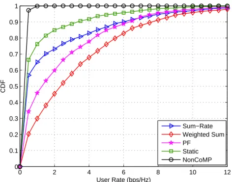
In Figure 2.6, the cumulative distribution function (CDF) of the capacity for the CoMP

re-questing users is plotted. The setup here is pcon _{= 16 dBW and γ = −8.3dB. The weighted}

sum dynamic scheme outperforms the others since it makes the users with low SINR to form

the CoMP cluster and hence reduces the most interference. The black line with circle marker is

the users whose SIN Rpilot _{< γ but there is no CoMP service available in the network, which is}

very poor compared with the other CoMP approaches.

Figure 2.7 is the CDF of the CoMP included users when the setup is the same as the one

in Figure 2.6. Seemingly, the sum-rate and the proportional fair schemes are better than the

weighted one. However, the reason is that they find the high SINR users to be the partners of

the CoMP requesting users. Note that if the SINR is already high, the effect of CoMP is limited

since the purpose of BS cooperation is to suppress interference. Therefore it is inefficient to

include users with high SINR in the CoMP cluster, even though it seems that the average rate of

the CoMP included users is increased.

Figure 2.8 plots the CDF of the last five percent users using the same setup as the one in

Figure 2.6. As mentioned above, we only observe the performance of the user in the central

cell. However, we can generate different samples of the user locations. For each sample, the

user capacity after running our BS clustering algorithms is calculated, and we sort the capacity

for all the samples and observe the ones with the lowest 5 % capacity. In general, the users with

such low capacity are located near cell-edge. So this figure shows the approximate performance

of the cell-edge users. It can be seen that the dynamic clustering scheme improves significant

fairness. The sum-rate approach provides less performance gain since it puts resource to the

0 2 4 6 8 10 12 0 0.1 0.2 0.3 0.4 0.5 0.6 0.7 0.8 0.9 1 User Rate (bps/Hz) CDF Sum−Rate Weighted Sum PF Static NonCoMP

Figure 2.6: The CDF of the CoMP requesting users.

0 2 4 6 8 10 12 0 0.1 0.2 0.3 0.4 0.5 0.6 0.7 0.8 0.9 1 User Rate (bps/Hz) CDF Sum−Rate Weighted Sum PF Static

0 0.05 0.1 0.15 0.2 0 0.1 0.2 0.3 0.4 0.5 0.6 0.7 0.8 0.9 1 User Rate (bps/Hz) CDF Sum−Rate Weighted Sum PF Static NonCoMP

Figure 2.8: The CDF of the last five percent users.

Figure 2.9 illustrates the effect of increasing the CoMP cluster size when the setup is the

same as the one in Figure 2.6. As expected, the average rate increases with the cluster size since

more interference is eliminated. The drawback is the raise of network overhead.

In Figure 2.10, the CDF of the weighted sum scheme versus different CoMP cluster size is

plotted when the setup is the same as the one in Figure 2.6. Only the performance of the CoMP

requesting users is observed. In addition to sum rate benefit, increasing the cluster size provides

3 3.5 4 4.5 5 5.5 6 6.5 7 4.6 4.8 5 5.2 5.4 5.6 5.8 6 6.2 6.4

CoMP Cluster Size

Average Rate (bps/Hz)

Sum−Rate Weighted Sum PF

Figure 2.9: The average rate versus different CoMP cluster size.

0 5 10 15 20 25 30 0 0.1 0.2 0.3 0.4 0.5 0.6 0.7 0.8 0.9 1 User Rate (bps/Hz) CDF

Weighted Sum, size = 3 Weighted Sum, size = 5 Weighted Sum, size = 7

Figure 2.10: The CDF of the CoMP requesting users using weighted sum utility versus different

CHAPTER 3

ADAPTIVE RESOURCE ALLOCATION

3.1

System Model and Transmission Schemes

In Chapter 2, we focus on a specific subcarrier and tackle the problem of BS clustering.

In this chapter, we extend the scenario to a more general multi-carrier system. Suppose some

CoMP clusters are formed in the cellular network based on a clustering algorithm. For the sake

of illustration, only one cluster is taken into consideration. Assume there are B BSs and K users

overall in this CoMP cluster, each BS equips Nt antennas and each user has Nr antennas. In

CoMP-JT mode, user data and CSI are shared across all the BSs in the same cluster, therefore,

a cluster is equivalent to a super BS with NT = BNt antennas which serves K users

simul-taneously. Let there are M available subcarriers, the downlink transmission can be illustrated

by Figure 3.1. In general, users are allocated to different subcarriers in order to avoid inter-user

interference. However, we can apply BD to decouple the channels of different users on the same

subcarrier. In this way, the spectral efficiency will be improved since multiple users can share

the same bandwidth.

Assume we place Km users on subcarrier m. After removing the cyclic prefix (CP) at the

user side, the signal can be processed in a per-subcarrier MIMO fashion. That is, the input-output

relation on every subcarrier can be represented in a MIMO structure. Ignoring the outer-cluster

interference, the received signal of the user k on the subcarrier m can be represented as

y_k,m = Hk,mxk,m+ Km

∑

n=1,n̸=k

Hn,mxk,m+ nk,m, (3.1)

where Hk,mis the Nr×NT MIMO channel, xk,mis the NT×1 transmitted signal for the user k and

nk,mis the zero-mean complex Gaussian noise vector with covariance matrix E

[

nk,m(nk,m) H]

=

N0INr. After BD (refer to section 2.1.1) pre-filtering, the transmitted signal can be represented

as

xk,m= Fk,mPk,mdk,m (3.2)

where Pk,m is the Nr × Nr power allocation matrix and dk,mis the Nr × 1 data vector before

pre-filtering. The BD matrix is Fk,m= Vk,meVk,m, where Vk,mmakes the channel of the user k

to be orthogonal to the channels of the others, and eVk,m decouples the orthogonalized MIMO

channel of the user k into Nrparallel SISO channels. Following the derivation similar to (2.24)

and (2.25), the lth_{spatial stream for the user k is}

rk,m,l = sk,m,l√pk,m,ldk,m,l+enk,m,l, 1≤ l ≤ Nr, (3.3)

where sk,m,l is the lthsingular value of the orthogonalized channel matrix of the user k on

sub-carrier m, pk,m,lis the power allocated on this stream, dk,m,lis the lthelement in dk,mandenk,m,l

is a zero-mean complex Gaussian noise with variance N0.

3.2

Problem Formulation

The mathematical problem of power minimization is formulated in this section. In order to

the transmit power while satisfies some constraints. In practice, users may have different QoS

requirements such as target data rate and tolerable BER. On the other hand, each antenna has its

own power amplifier and therefore has a unique transmit power constraint. Considering all the

issues above, the power minimization problem can be formulated as

minimize pk,m,l K ∑ k=1 M ∑ m=1 Nr ∑ l=1 pk,m,l subject to M ∑ m=1 Nr ∑ l=1 rk,m,l ≥ Mrtark , 1≤ k ≤ K K ∑ k=1 M ∑ m=1 Nr ∑ l=1 |Fk,m[a, l]| 2 pk,m,l ≤ pcona , 1≤ a ≤ NT pk,m,l ≥ 0, ∀k, m, l, (3.4)

where pk,m,l and rk,m,l is the transmit power and rate allocated on the lth stream of the user k

on the subcarrier m, r_ktar is the target data rate in bps/Hz, Fk,m[a, l] is the element in the ath

row and lth_{column of the BD matrix F}

k,m, and pcona is the power constraint on transmit antenna

a. Note that if the bandwidth of each subcarrier is β, the total rate requirement per user of one OFDM symbol is M βrtar_k (bps), therefore, M rtar_k bits are required during the period of one OFDM symbol. The rate rk,m,lcan be written as

rk,m,l = log2 ( 1 + pk,m,ls 2 k,m,l τ N0 ) , (3.5)

where τ is the SNR gap given by

τ =−ln (5BER

tar₎

1.5 , (3.6)

where BERtar_{is the target BER specified by the users. Although the capacity is hard to achieve}

in practice, it provides an upper bound that tells us how well we can do. The problem (3.4)

implies a user selection problem on each subcarrier. If pk,m= Nr

∑

l=1

pk,m,l = 0, the user k is absent

modified version of the one in [12], which considers no power constraint. However, as the user's

target rate increases, the minimized power may exceed the transmit power limit. Therefore, we

want to see how the results will be when the per-antenna power constraints are added to the

power minimization problem.

3.3

Low Complexity Solution for Power Minimization

3.3.1

Optimization Based on Dual Decomposition

In this section, we propose a low complexity solution to (3.4) based on the Lagrange dual

transformation. For the sake of interpretation, we rewrite (3.4) in a new form:

minimize r f (r) subject to M ∑ m=1 rm ≽ Mrtar g (r)≼ pcon, (3.7) where r =[rT₁, . . . , rT m, . . . , rTM ]T , with rm = [r1,m, . . . , rk,m, . . . rK,m]T, with rk,m = Nr ∑ l=1 rk,m,l

are the allocated rates, rtar= [rtar₁ , . . . , rtar_K]T are the target rates, pcon =[pcon₁ , . . . , pcon_N

T

]T

are the

per-antenna power constraints, f (·) and g (·) are the RM K _{→ R and R}M K _{→ R}NT _mapping

functions, respectively, and a ≽ b means ai ≥ bi, ∀i. The constraints pk,m,l ≥ 0, ∀k, m, l in

(3.4) are removed temporarily and will be considered afterwards (in Appendix A.1). Although

the original objective function f (·) is not convex, it can be transformed into a dual function, which is always concave regardless of the convexity of f (·). Hence traditional convex opti-mization techniques can be used to solve the transformed problem. We start from the Lagrangian

of (3.7), which is L (r, µ, κ) = f (r) + µT ( M rtar− M ∑ m=1 rm ) + κT (g (r)− pcon) , (3.8)

where µ = [µ1, . . . , µK] T

and κ = [κ1, . . . , κNT] T

are the vectors of Lagrange multipliers

correspond to the rate and power constraints in (3.7). The dual function is defined as

d (µ, κ) =L (r∗, µ, κ) , (3.9) where r∗ = min

r L (r, µ, κ). The dual problem can be formulated as

maximize

µ,κ d (µ, κ)

subject to µ≽ 0

κ≽ 0. (3.10)

In another word, we let the Lagrange multipliers to be constants temporarily and find the r∗ which minimizes the LagrangianL (r, µ, κ), this is the definition of the dual function d (µ, κ). Next, we formulate the dual problem which aims to find the optimal Lagrange multipliers that

maximize the dual function. In contrast with the dual problem, the original problem (3.7) is

called the primal problem. The dual problem is equivalent to the primal problem if the original

objective function f (·) is convex, otherwise, there exists a duality gap between these two prob-lems [18]. In our case, f (·) is not convex since it is a pointwise minimum of several convex functions. Nevertheless, [19] shows that this gap can be reduced by increasing the subcarrier

size M . In order to find the r∗ in (3.9), we first express (3.8) in another form: e L = K ∑ k=1 M ∑ m=1 Nr ∑ l=1 pk,m,l+ K ∑ k=1 µk ( M rtar_k − M ∑ m=1 Nr ∑ l=1 rk,m,l ) + NT ∑ a=1 κa ( _K ∑ k=1 M ∑ m=1 Nr ∑ l=1 |Fk,m[a, l]| 2 pk,m,l− pcona ) . (3.11)

Since data rate is a function of power, therefore, finding the r∗which minimizesL is equivalent to finding p∗_k,m,l, ∀k, m, l which minimize eL, so we set the latter to be our new goal. After making some arrangements to (3.11), it becomes

e L = M ∑ m=1 K ∑ k=1 Nr ∑ l=1 ( L (m, k, l))+ K ∑ k=1 µkM rtark − NT ∑ a=1 κapcona , (3.12)

where L (m, k, l) = pk,m,l− µkrk,m,l+ NT ∑ a=1 κa|Fk,m[a, l]|2pk,m,l. (3.13)

In the dual function, µk and κa are treated as constants temporarily, so the last two terms in

(3.12) are unrelated terms. Therefore, minimizing eL is equivalent to minimizing L. On each subcarrier, when the user selection has been determined, we can obtain the BD precoding

ma-trices Fk.m, ∀k, m, the minimal power and rate allocated on each spatial stream can be given

by pk,m,l = max          µk ln (2) 1 1 + NT ∑ a=1 κa|Fk,m[a, l]|2 − τ N0 s2 k,m,l , 0          (3.14) and rk,m,l= log2     max          µks2k,m,l ln (2) τ N0 ( 1 + NT ∑ a=1 κa|Fk,m[a, l]|2 ), 1              . (3.15)

For brevity, the derivations of (3.14) and (3.15) are left in Appendix A.1. We call this solution

the competitive water-filling solution. The reason for the name will be explained later.

Since BD can mitigate the inter-user interference on the same subcarrier, multiple users can

share the same bandwidth. The optimal user selection on each subcarrier would be to search

over 2K_{user combinations and find the one that minimizes}

b L (m) = K ∑ k=1 Nr ∑ l=1 L (m, k, l). (3.16)

For the overall M subcarriers, there would be M 2K choices. As mentioned above, the duality gap approaches zero when M goes to infinity. However, this will make user selection problem

to be computational infeasible. The complexity could be reduced by a suboptimal greedy user

selection introduced in [12]: For each subcarrier, allocate the user that minimizes bL (m) on subcarrier m. Next, add another one from the remaining K − 1 users if bL (m) can be further reduced, and so on. Note that if bL (m) ≥ 0, there is no user allocated on this subcarrier, since

positive bL (m) will not minimize eL. As the number of users on this subcarrier increases, the BD precoder will project each user's channel to a more restricted space (see section 2.1.1), which

makes the channels weak. Hence, it is not always the best to put all the users on each subcarrier,

even though they do not interfere to each other after BD. The suitable number of users that

allocated on each subcarrier can be found by the greedy user selection algorithm above. In this

way, the maximum combination of users over the total M subcarriers becomes M

K∑−1 j=0 (_K−j 1 ) = M K(K+1)

2 , which is small compared to M 2

K _{when K is large. As for the globally optimal}

solution, even if the per-antenna power constraints are ignored and the minimal power which

satisfies the user rate constraint is obtained by the water-filling solutions (which are (3.14) and

(3.15) after setting κa= 0, ∀a), it still needs a search over 2KM possibilities to find the optimal

solution, which is computationally prohibitive.

So far, we have found the p∗_k,m,l, ∀k, m, l that minimize eL and therefore the dual function d (µ, κ) is obtained. Next, we need to find the optimal µ and κ that maximize d (µ, κ). Since d (µ, κ) is concave, we can update µ and κ along some directions to find the optimal point. We adopt a special searching direction named supergradient [20]. In general, the supergradient at a

point α∈ Rn×1 is defined as a vector χ∈ Rn×1which satisfies

d (α)e ≤ d (α) + χT (αe − α) , ∀eα̸= α. (3.17) In our optimization problem (3.7), α comprises the Lagrange multiplier vectors µ and κ, and

χ can be decomposed into two directions χ₁and χ₂, which are given by

χ₁ = M rtar− M ∑ m=1 r∗_m (3.18) and χ₂ = g (r∗)− pcon, (3.19) where g (·) is the function defined in (3.7). The proofs are shown in Appendix A.2. Without

changing the direction, we divide the first supergradient by M , that is, χ₁ = χ₁/M =[χ_1,1, . . . , χ_1,k, . . . , χ_1,K]T, (3.20) where χ_1,k = r_ktar− 1 M M ∑ m=1 Nr ∑ l=1 rk,m,l. (3.21)

The second supergradient remains the same, which is

χ₂ = [χ2,1, . . . , χ2,a, . . . χ2,NT] T (3.22) where χ2,a = K ∑ k=1 M ∑ m=1 Nr ∑ l=1 |Fk,m[a, l]| 2 pk,m,l− pcona . (3.23)

We update the two Lagrange multiplier vectors in an iteration manner:

µi+1_k = max{µi_k+ δ₁iχ_1,k, 0} (3.24) and

κi+1_a = max{κi_a+ δi₂χ2,a, 0

}

, (3.25)

where i is the iteration index, δi

1 and δ2i are the two positive step sizes for µ and κ, respectively.

As we can see in (3.21), if the allocated rate to the user k exceeds the its target, the direction

becomes negative and µkwill be reduced in the next iteration. On the contrary, µkwill increase

if it falls below the target rate. The similar actions can be observed in (3.23). Since the rate

(3.15) is directly proportional to µkbut inversely proportional to ϕa, consider a case that a user

requests so much rate that the allocated power goes beyond the per-antenna power constraints,

then χ₂becomes positive and hence increases κ, as a consequence, the power will be dropped.

However, it will be raised again since the target rates are not satisfied due to insufficient power.

This causes a struggle situation in our iterative algorithm and that is why the allocation scheme is

much or the power constraints are set to very high, the allocated rate to each user will gradually

converge to their targets from an initial point without struggling.

3.3.2

Convergence Behavior Control

In this section, we design the initial point and step size for a faster convergence. Although

the concavity of the dual function promises that the power and rate will converge along the

supergradient, we can boost the speed of convergence by finding the proper initial values. The

choice of the step size also has great impacts. A small step size lengthens the convergence time,

while a large step size leads to coarse convergence result. The main design principle in this

section is based on [12]. In order to give the initial values of µ and κ, we let each subcarrier

is occupied by all the K users and BD is deployed to separate the users. Even though this is

not the optimal way, it gives a good starting point to our algorithm. Since the user selection has

been fixed now, we can apply the competitive water-filling solution (3.14) and (3.15), where the

initial values of κ0

a, ∀a are generated uniformly on an open interval (0, 1), and the initial values

of µ0

k, ∀k are chosen to the levels such that M ∑ m=1 Nr ∑ l=1 rk,m,l = M rktar, ∀k. (3.26)

The initial step sizes for updating µ and κ can be designed as

δ₁0 = η1 K ∑ k=1 µ0 k K ∑ k=1 rtar k (3.27) and δ₂0 = η1 NT ∑ a=1 κ0 a NT ∑ a=1 pcon a , (3.28)

where η1 > 0 is a constant. There are two behavior when the algorithm is running, the first is

that µ and κ are changing in one direction, which can be expressed as

sign(χi_1,k) == sign(χi_1,k−1), ∀k (3.29) and

sign(χi_2,a)== sign(χi_2,a−1), ∀a, (3.30) where “==" is the equality judgment. Since the initial values may be far from the optimal

results, this situation tells us the µ and κ are approaching the optimal values. Therefore, we can

increase the step sizes to boost the convergence by adjusting

δ₁i+1= η2δi1 (3.31)

and

δ₂i+1= η2δ2i, (3.32)

where η2 > 1 is a constant. On the other hand, if µ and κ are oscillating, which means that they

are already close to the optimal values. The oscillation behavior can be represented as

∃k such that [sign(χi_1,k) ̸= sign(χi_1,k−1)]∩[sign(χi_1,k−1)̸= sign(χi_1,k−2)], (3.33) and the second direction is

∃a such that [sign(χi_2,a)̸= sign(χi−1_2,a)]∩[sign(χi−1_2,a)̸= sign(χi−2_2,a)]. (3.34) In this case, we can stabilize them by changing

δ₁i+1= δ₁i/η3 (3.35)

and

where η3 > 1 is a constant. If the condition does not belong to anyone of these two, then δi1and

δi

2 remain the same. Besides, in order to prevent the step size from going unboundedly. We set

the upper and lower bounds for the step size, which are

δ₁(max) = η(max)δ0₁, δ(max)₂ = η(max)δ₂0 (3.37)

and

δ₁(min) = η(min)δ₁0, δ₂(min) = η(min)δ₂0. (3.38)

where η(max) > 1 and 0 < η(min) < 1 are constants.

It should be noted that although the behavior of µ and κ have some relation, but they are not

fully identical. In other words, if µ is moving in one direction, it is possible that κ is oscillating.

In short, our resource allocation algorithm can be illustrated by Figure 3.2.

Fixed user selection, get initial and

Clear all the users on each subcarrier Adaptive user selection and resource allocation Max iteration? Compute supergradient Update and End No Yes