Microstructure Dynamics and Agent-Based
Financial Markets
Shu-Heng Chen1, Michael Kampouridis2, and Edward Tsang2
1 AI-ECON Research Center, Department of Economics, National Chengchi
University, Taiwan chen.shuheng@gmail.com
2 School of Computer Science and Electronic Engineering, University of Essex, UK
Abstract. One of the essential features of the agent-based financial models is to show how price dynamics is affected by the evolving mi-crostructure. Empirical work on this microstructure dynamics is, how-ever, built upon highly simplified and unrealistic behavioral models of financial agents. Using genetic programming as a rule-inference engine and self-organizing maps as a clustering machine, we are able to recon-struct the possible underlying microrecon-structure dynamics corresponding to the underlying asset. In light of the agent-based financial models, we further examine the microstructure both in terms of its short-term dynamics and long-term distribution. The time series of the TAIEX is employed as an illustration of the implementation of the idea.
1
Introduction and Main Ideas
It comes as no surprise to economists that there is no single strategy which can persistenly dominate all other strategies in the market. The idea of the best strategy is simply inconsistent with the intuitive notion of the efficient market hypothesis. While this feature is well expected among economists, the result shown by [7], generally known as the overreaction hypothesis, is still very appealing. They have found that successive portfolios formed by the previous five years’ 50 most extreme winners considerably underperform the market average, while portfolios of the previous five years’ 50 worst losers perform better than the market average.3
Recently, a similar phenomenon has been rigorously analyzed and replicated in the agent-based finance literature, in particular, in the H-type model. In this literature, markets at any point in time are composed of different clusters (types) of agents. Agents who follow similar rules are considered to be in the same cluster. Each cluster is defined by the associated behavioral rules. The market microstructure is characterized by the fractions (distribution) of individuals over different clusters. Different distributions (microstructure) over the clusters may have different impacts on the aggregates, and both the microstructure and the aggregates are evolving with feedbacks to each other.
3 The overreaction hypothesis has been extensively examined in the finance literature.
Complex dynamic analysis of these models indicates two interesting proper-ties. First, in the short run, it is likely that the market fractions are constantly changing. In particular, for each cluster, the market fraction can swing from very low to very high, i.e., switching between the majority and the minority. Second, in the long run, no single strategy can dominate the other, i.e., the mar-ket fraction converges to 1/H for each cluster. These two properties provide us with a basis to study the complex dynamics of microstructure, which we refer to together as the market fraction hypothesis, or as an abbreviation, the MFH. In fact, a number of empirical studies have already attempted to estimate the parameters associated with the MFH [5].
This paper, however, differs from the H-type models in two regards. First, we do not assume any prefixed behavioral rule (functional form) for any clus-ter (type) of agents; second, we do not assume that agents of the same type are homogeneous, while they can be similar. We consider that this departure will lead us to a more general and realistic implication of the MFH. Consider the three-type model as an example. In the fundamentalist-chartist-contrarian model, traders of the same type at any point in time behave in exactly the same way, and their functional forms of behavioral rules, in this case, their forecasts of the price in the next period, {Ef,t(pt+1)}, {Ec,t(pt+1)} and {Eco,t(pt+1)}, are
all known. Equations (1) to (3) are typical examples.
Ef,t[pt+1] = pt+ αf(pft − pt), 0 ≤ αf ≤ 1, (1)
Ec,t(pt+1) = pt+ αc(pt− pt−1), 0 ≤ αc. (2)
Eco,t(pt+1) = pt+ αco(pt− pt−1), αco≤ 0. (3)
Nevertheless, in the real world, the behavioral rules of each trader are expected to be heterogeneous, and even if they can be clustered into types, the representative behavior of each type is normally unknown.4
1.1 Genetic Programming as a Rule-Inference Engine
In this paper, we assume that traders’ behavior, including price expectations and trading strategies, is either not observable or not available. Instead, their behavioral rules have to be estimated by the observable market price. Using macro data to estimate micro behavior is not new as many H-type empirical agent-based models have already performed such estimations [5]. However, as mentioned above, such estimations are based on very strict assumptions upon which a formal econometric model can be built. Since we no longer keep these assumptions, an alternative must be developed, and in this paper we recommend genetic programming (GP).
4 While the ideas of fundamentalists and chartists are the results of field work,
ab-stracting the general observed behavior into a very specific mathematical model is a big leap.
The use of GP as an alternative is motivated by considering the market as an evolutionary and selective process.5In this process, traders with different
behav-ioral rules participate to the markets. Those behavbehav-ioral rules which help traders gain lucrative profits will attract more traders to imitate, and rules which result in losses will attract fewer traders.6This evolutionary argument in fact is,
intu-itively, the same as the evolution process considered by the H-type agent-based financial models. For example, their use of the Gibbs-Boltzman distribution is a formalization of this process. Genetic programming is another formalization which, unlike the former, does not rest upon any pre-specified class of behavioral rules. Instead, in GP, a population of behavioral rules is randomly initiated, and the survival-of-the-fittest principle drives the entire population to become fitter and fitter in relation to the environment. In other words, given the non-trivial financial incentive from trading, traders are aggressively searching for the most profitable trading rules. Therefore, the rules that are outperformed will be re-placed, and only those very competitive rules will be sustained in this highly competitive search process.7
Hence, even though we are not informed of the behavioral rules followed by traders at any specific time horizon, GP can help us infer what these rules are approximately by simulating the evolution of the microstructure of the market. Without imposing tight restrictions on the inferred behavioral rules, GP enables us to go beyond the simple but also unrealistic behavioral rules used in the H-type agent-based financial models. Traders can then be clustered based on more realistic, and possibly more complex behavioral rules.8
1.2 Self-Organizing Maps as a Clustering Machine
Once a population of rules is inferred from GP, it is desirable to cluster them based on a chosen similarity criterion so as to provide a concise representation of the microstructure. The similarity criterion which we choose is based on the observed trading behavior. Based on this criterion, two rules are similar if they are observationally equivalent or similar, or, alternatively put, they are similar if they generate the same or similar market timing behavior.
Given the criterion above, the behavior of each trading rule can be repre-sented by its series of market timing decisions over the entire trading horizon,
5 See [18] for his eloquent presentation of the adaptive market hypothesis.
6 One may wonder how traders can imitate each others’ rules by having a sample of
behavior but not the rules underlying it. This question has been addressed in [4], where they proposed a mechanism called business school to show how the seemingly unobservable rules can be imitated.
7 It does not necessarily mean that the types of traders surviving must be smart
and sophisticated. They can be dumb, naive, randomly behaved or zero-intelligent. Obviously, the notion of rationality or bounded rationality applying here is ecological [21, 11].
8 [9] provides the first illustration of using genetic programming to infer the behavioral
rules of human agents in the context of ultimatum game experiments. Similarly, [12] uses genetic algorithms to infer behavioral rules of agents from market data.
for example, 6 months. Therefore, if we denote the decision “enter the market” by “1” and “leave the market” by “0”, then the behavior of each rule is a binary string or a binary vector. The length of these strings or the dimensionality of the vectors is then determined by the length of the trading horizon. For example, if the trading horizon is 125 days long, then the dimension of the market timing vector is 125. Once each trading rule is concretized into its market timing vec-tor, we can then easily cluster these rules by applying Kohonen’s self-organizing maps (SOMs) [15] to the associated clusters.
The main advantage of SOMs over other clustering techniques such as K-means is that the former can present the result in a visualizable manner so that we can not only identify these types of traders but also locate their 2-dimensional position on a map, i.e., a distribution of traders over a map. Furthermore, if we suppose that we do not have dramatic crustal plate movement so that the map is fixed over time, then the distribution of traders over the map can, in effect, be comparable over time. This provides us with a rather convenient grasp of the dynamics of the microstructure directly as if we were watching the population density on a map over time.
However, the assumption of crustal stability does not hold in general; there-fore, maps over time are not directly comparable. To make them comparable, some adjustments are needed. The idea of adjustment is also very intuitive. If the dominant strategy remains unchanged from period A to period B, then when we apply the dominant trading strategy derived from period A to another pe-riod B, the strategies should behave in a way that is similar to the dominant strategy derived from period B, if it is not exactly the same. This motivates us to emigrate all trading strategies from one map (the home map) to the other (the host map) in such a way that each emigrant shall find its new cluster on the host map based on the same similarity metric. In this manner, we can recon-struct a time-invariant version of the map, and comparison can be made upon this reconstruction.
The rest of the paper is organized as follows. Section 2 provides a brief description of the version of genetic programming used in this paper. Section 3 demonstrates the self-organizing map constructed based on the description in Section 1.2. A time series of these maps is constructed accordingly and the maps are then analyzed both in their short-term dynamic behavior (Section 3.1) and long-term distribution behavior (Section 3.2). The analysis is further consolidated with the results from multiple runs (Section 3.3). Section 4 examines the short-term dynamics and long-term distribution behavior of a rather small self-organizing map. In Section 5, we present our concluding remarks.
2
Genetic Programming
In this paper, we use the financial GP system introduced by Edward Tsang at University of Essex, known as Eddie. Eddie, standing for Evolutionary Dynamic Data Investment Evaluator, applies genetic programming to evolve a population of artificial financial advisors or, alternatively, a population of market-timing
<Tree> ::= If-then-else <Condition> <Tree> <Tree>| Decision
<Condition> ::= <Condition> “And” <Condition>|
<Condition> “Or” <Condition>|
”Not” <Condition>|
VarConstructor <RelationOperation> Threshold
<Variable> ::= MA 12| MA 50 | TBR 12 | TBR 50 | FLR 12 |
FLR 50| Vol 12 | Vol 50 | Mom 12 | Mom 50 |
MomMA 12| MomMA 50
<RelationOperation> ::= “>”| “<” | “=”
Decision is an integer, Positive or Negative implemented Threshold is a real number
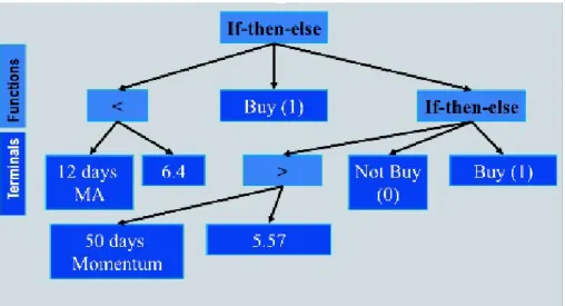
Fig. 1. The Backus Normal Form of EDDIE
strategies, which guide investors on when to buy, to hold, or to sell. These artificial financial agents (market timing strategies) are formulated as decision trees in Eddie, which, when combined with the use of GP, are referred to as Genetic Decision Trees (GDTs).
Each of these market-timing strategies (GDTs) is syntactically (grammati-cally) produced by the Backus Normal Form (BNF) [3]. Figure 1 presents the Backus Normal Form (BNF) of the GP. As we can see, the root of the tree is an If-Then-Else statement. Then the first branch is a boolean (testing whether a technical indicator is greater than/less than/equal to a value). The ‘Then’ and ‘Else’ branches can be a new Genetic Decision Tree (GDT), or a decision, to buy or not-to-buy (denoted by 1 and 0).
What is also shown in Figure 1 is a list of major terminals (technical indi-cators) used for growing our GDTs. These terminals are moving average (MA), trade break-out rule (TBR), filter (FLR), volatility (Vol), momentum (Mom), momentum moving average (MomMA). The GDTs generated from these termi-nals under the BNF are very similar to those generated in [1, 6, 19]. Also see Figure 2 below.
The fitness function used to evolve GP is mainly built upon the confusion matrix [20], which is presented in Table 1. Each point in time, each GDT makes a recommendation to buy (positive prediction) or not to buy (negative prediction). We call a decision (prediction) to buy true positive if it leads to a positive profit, and false positive if it leads to a negative profit. Similarly, a decision not to buy is called true negative if it helps to avoid a negative profit and is called false negative if it causes investor to miss a profitable opportunity.
Table 1. Confusion Matrix
Actual Positive Actual Negative
Positive Prediction True Positive (TP) False Positive (FP) Negative Prediction False Negative (FN) True Negative (TN)
With this matrix, we can develop the following three metrics: Rate of Correctness
RC = T P + T N
T P + T N + F P + F N (4)
Rate of Missing Chances
RM C = F N
F N + T P (5)
Rate of Failure
RF = F P
F P + T P (6)
Li [17] combined the above metrics and defined the following fitness function: f f = w1∗ RC − w2∗ RMC − w3∗ RF (7)
where w1, w2 and w3 are the weights for RC, RMC and RF respectively. These
weights are given in order to reflect the preferences of investors. For instance, a conservative investor would want to avoid failure; thus a higher weight for RF should be used. However, tuning these parameters does not seem to affect the performance of the GP [17]. For our experiments we chose to include strategies that mainly focus on correctness and reduced failure. Thus these weights have been set to 1, 1/6 and 1/2 respectively.
Table 2 presents other GP parameters for our experiments. The GP param-eters for our experiments are the ones used by Koza [16]. Only the tournament size has been changed (lowered), and the reason for that was because we were observing premature convergence. Other than that, the results seem to be in-sensitive to these parameters.
Table 2. Tableau of GP Control Parameters. GP Parameters
Max Initial Depth 6
Max Depth 17 Generations 50 Population size 500 Tournament size 2 Reproduction probability 0.1 Crossover probability 0.9 Mutation probability 0.01 {w1, w2, w3} {1, 1/6, 1/2}
Given the fitness function above and a set of historical data, GP is then applied to evolve these market-timing strategies in a standard way. After evolving
Fig. 2. An Example of Genetic Decision Trees
a number of generations, what stands (survives) at the end (the last generation) is, presumably, a population of financial agents whose market-timing strategies are financially rather successful. An example of one best fitted GDT is given in Figure 2.
3
An Illustration from the Taiwan Stock Market
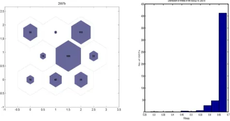
Figure 3 gives a concrete illustration of the idea presented above (Sections 1.1 and 1.2). Here, 500 artificial traders are grouped into nine clusters. The parameter value ‘500’ refers to the population size used in genetic programming, i.e., the rule-inference stage, whereas the parameter value ‘9’ is due to a 3 × 3 two-dimensional SOM employed in the rule clustering stage. In a sense, this could be perceived as a snapshot of a nine-type agent-based financial market dynamics. Traders of the same type indicate that their market timing behavior is very similar. The market fraction or the size of each cluster can be seen from the number of traders belonging to that cluster. Not surprisingly, they are not evenly distributed. Figure 3 shows that the largest cluster has a market share of 37.6% (188/500), whereas the smallest cluster has a market share of only 0.4% (2/500). Once we can have a snapshot of the market fraction, we can go further over a series of snapshots so as to have a picture of the dynamics of the market fraction or the dynamics of the market microstructure. However, as we mentioned before, the SOMs constructed from different periods are not directly comparable; therefore, to make them all comparable, we have to first choose a base period and
0.250 0.3 0.35 0.4 0.45 0.5 0.55 0.6 0.65 0.7 50 100 150 200 250 300 350 400 450
Distribution of fitness of the 500GDTs: 2007b
Fitness
No of GDTs
Fig. 3. 3× 3 Self-Organizing Feature Map
The left panel shows the SOM constructed based on the 500 financial decision trees generated by GP using the daily data of the TAIEX from July 2007 to December 2007. The right panel gives the associated histogram of the fitness of these 500 GDTs.
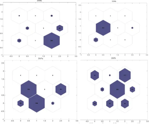
fix the map, i.e., to take the centroid of each cluster as given. In this particular example, we choose the second half of the year 2007 as the base. Once the centroids are given, all points (vectors) in other maps shall immigrate into this fixed map, and they are re-clustered based on their similarity to these fixed centroids. Figure 4 shows the reconstruction of these maps in this manner.
This figure has the market fraction maps from the year 2006 to the year 2007, crossing 4 different periods.9 These maps were constructed by using the second
half of 2007 as the base period. This figure gives a clear picture of what we mean by market fraction dynamics. First of all, we notice that the distribution over the clusters is uneven over time. In each period of time, some clusters obviously dominate others, but that dominance changes over time. This can be seen from the constant renewing of the major blocks. This eye-browsing inspection mo-tivates us to formulate two hypotheses which we already experienced from the dynamics of H-type agent-based financial models.
3.1 Short-Term Dynamics
The first hypothesis regards the short-run dynamics of market fraction. Each type of trader can be a dominant group (majority) for some of the time, but the duration of its dominance can only be temporal. The quick turnover of the dominant cluster or its short duration is consistent with the impression of the
9 We, of course, have a total of 34 maps from the year 1991 to the year 2007, and it
Fig. 4. Market Fraction Dynamics: Map Dynamics
The four SOMs above are constructed using the daily data of the TAIEX from 2006 to 2007. From the top-left panel to the bottom-right panel, they correspond to the first half and seconf half of year 2006 (2006a, b) and the first half and second half of the year 2007 (2007a, b). Except for the last one, 2007b, the other three are reconstructed by using 2007b as the base (see Section 1.2).
swinging dynamics as we saw in the 2-type agent-based financial models, e.g., [14]. However, in addition to eye-browsing the swing, it is desirable to have an objective measure of how persistent a dominant cluster can be. To do so, we need an operational meaning of dominance. Even though there is no unique way of doing this, we find the following threshold to be quite general and useful.
¯q = 1 + p
H + p, (8)
where H is the number of clusters, and p, a non-negative integer, is a control parameter for the degree of dominance. Hence, a cluster is dominant if its market fraction exceeds this threshold. By varying the parameter p, one can therefore have an operational meaning that is consistent with our intuition regarding dom-inance. For example, if H = 2 (a two-type model) and p = 2, a cluster can be
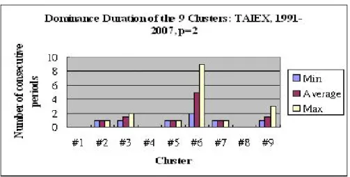
Fig. 5. Duration of Dominance (p=2)
dominant only if its market fraction is greater than a ¯q of 75%, a standard much higher than just breaking the tie (one half). Of course, the higher the p, the higher the threshold.
Figure 5 presents the dominance-duration statistics of each type of trader. Basically, we keep track of the persistent time of each dominance. Once after a type of trader become dominant, we count how many periods in a row that it can remain the dominant cluster. Figure 5 gives three statistics regarding du-ration, namely, minimum, average and maximum. For example, for Cluster Six, these three statistics are 1, 3 and 9, respectively. In other words, the maximum duration of dominance for Cluster Six is about nine periods, i.e., four and a half years. For other clusters, the longest duration is no more than three periods, i.e, one and half years. So, for most of the time, dominant clusters can hardly continue for long. Hence, we reach the conclusion that, regardless of the types of traders, we can rarely see the consecutive dominance. In this sense, our data lend support to the market fraction hypothesis in a weak sense.
3.2 Long-Term Distribution
The second hypothesis which we can form regarding the market fraction behavior is its long-term distribution. Many H-type agent-based financial models can show us that, under some proper parameter values, the long-term market fraction is even. In other words, if we have H types of traders, their long-term frequency of appearance should be close to 1
H. Let Cardi,t be the number (cardinality) of
traders in Cluster i in time period t.
H
!
i=1
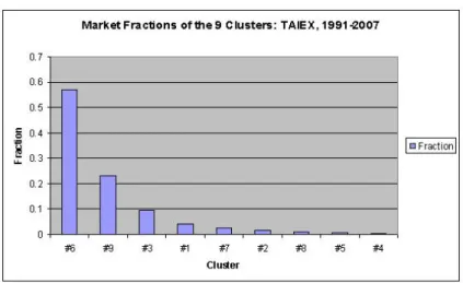
Fig. 6. Long-Term Histogram
In our current setting, N, the total number of traders, is 500. The long-term histogram can be derived by simply summing the number of traders over all periods and dividing it by a total of N × T (# of periods),
ωi=
"T
t=1Cardi,t
N× T . (10)
Figure 6 gives the long-term histogram of these clusters, {ωi}. Obviously,
they are not equal so that we present them in descending order from the left to the right. Cluster Six has the largest market fraction up to almost 60%, whereas Cluster 4 has the smallest market fraction, which is not even up to 1%.
Of course, this distribution is very different from the uniform one. In order to give a measure of how far it is from the uniform one, we use the familiar entropy as a metric. For the discrete random variable, the entropy is defined as
Entropy =−
H
!
i=1
piln pi, (11)
where piis the fraction of each cluster. Let us denote the empirical distribution
presented in Figure 6 as fX, and the uniform distribution as fY. By definition,
fY = H1, where H is the number of clusters, which in this case is 9. In order
to measure how close fX is to the uniform distribution fY, we calculate the
entropy of both distributions. It is well known that for the uniform distribution Entropy(Y ) = ln H. When H=9, it is ln 9 ≈ 2.2. The closer Entropy(X) is to 2.2, the closer X is to the uniform distribution. After calculating X’s entropy, we find it equal to 1.3, which is only 59% of the entropy of the uniform distribution.
Table 3. Summary Results over 10 runs, for a 3×3 SOM.
Short-Run Long-Run
Mean Max E-Ratio
TAIEX (9 Clusters) 2.02 8.25 0.55
TAIEX (3 Clusters) 4.05 8.14 0.80
Summary As we have seen in this section and the previous one, both the short-run and the long-run version of the market fraction hypothesis are not well supported. The short-run dynamics indicates the appearance of a long-lasting dominant cluster (up to a maximum of 9 periods). On the other hand, the long-run histogram is very far away from the uniform distribution.
3.3 Results from Multiple Runs
However, so far we have only presented the results of a single run. To consolidate our results, we further replicate the experiments for an additional nine runs, and Table 3 gives the results for ten runs together.
The first two numeric columns are related to the short-run dynamics and present the averages over the 10 runs for both the average duration and the maximum duration of the 9 clusters. This result is not much different from our earlier single-run results. The mean dominance duration over these ten runs is just about 2 (one year). Nevertheless, the existence of few long-lasting dominant clusters is very evident with the mean maximum duration reaching as high as 8.25 periods (more than 4 years). Hence, the short-run version of the market fraction hypothesis is only weakly supported. The next column presents the ratio of the average realized entropy (over the 10 runs) relative to the base entropy under the null of the uniform distribution, which is 55%, and still quite far away from one. Therefore, the long-term version of the market fraction hypothesis is not well supported.
4
Does the Number of Types Matter?
The illustration presented above is based on a 3 by 3 SOM, which automatically generates nine clusters. This analysis has its limitations mainly because we do not know how many types of agents are really there in the market. In a rather theoretical analysis, [2] showed that it would be enough to characterize the mar-ket behavior by a few types, say two to three. Others are rather marginal.10
10Aoki [2] is probably the only paper known to us that deals with number of types
of agents in the multi-agents system. Using the Ewens-Pitman-Zabell induction method, Aoki applies the result from the evolution of biological species and pop-ulation genetics to determine the minimum number of types of behavior required
Therefore, it would be interesting to investigate the microstructure dynamics based on a smaller SOM corresponding to the few-type agent-based financial models.11
In this section, we therefore repeat the above experiments by using a rather small 3 × 1 SOM. We then examine both its short-term dynamics and the long-term histogram. As before, we have 10 multiple runs. The results are shown in Table 3. In terms of duration behavior, we can see that there is no significant difference in the maximum duration between the 9-cluster case and the 3-cluster case, for here the mean maximum duration is consistently a little above eight (four years). However, a significant difference in mean duration does exist. What we find here is that when the number of clusters decreases, the mean duration increases from the original 2.02 periods (one year) to 4.05 periods (two years). Therefore, it seems that a smaller number of clusters really drives the short-run dynamics further away from the expectations of the market fraction hypothesis. On the other hand, if we look at the long-term distribution behavior, we find that a smaller number of clusters does help the distribution (histogram) get closer to the uniform distribution. As shown in Table 3, the realized entropy ratio now increases up to 80% from the original 55%. Hence, the market fraction hypothesis is better supported from a long-term point of view.
Putting them together, what we have observed here is that, when the number of clusters gets smaller, the dominant cluster maintains its position longer, but a different cluster does take the lead in turn, and so, in the long run, they are better tied.12
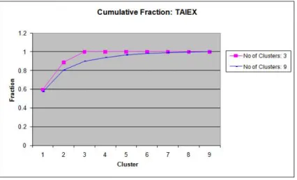
If the number of clusters does matter for the microstructure dynamics, then it is imperative to know how many clusters we need. To answer this question, Figure 7 presents the cumulative fraction sum from the largest cluster to the smallest cluster. For the 3-cluster case, when the number of clusters (the x axis) gets to 3, the cumulative fraction becomes one, and similarly for the 9-cluster case when the number of clusters gets to 9. However, what we can see here is that when coming to the first five clusters, there is already an accumulation of 96% of the market share. In fact, if we care only about 90% of the market fraction, then 3 clusters are sufficient.
5
Concluding Remarks
After a decade of development, the literature on agent-based financial models has successfully demonstrated the connection between microstructure dynamics
to capture multi-agent economic systems. He showed that when agent behavior are positively correlated, two largest clusters are likely to develop to which most agents belong. This result, therefore, provides some justification for studying economic mod-els composed of many interacting agents of two or three strategy types.
11Based on [5], the 2-type or the 3-type agent-based financial models are still the most
popularly-used classes in the literature.
12To see how significant or how interesting this pattern is, Monte Carlo simulation
is conducted, and the patterns obtained are significantly different. Due to the size limit of the paper, details are not provided here, but are available in [13].
Fig. 7. Cumulative Fractions of 3 Clusters and 9 Clusters
and asset price dynamics. The next research agenda would be to gain more understanding of the empirical properties of this microstructure dynamics. In this paper we have shown that the number of types (clusters) of agents may be limited, but the duration of dominant groups are larger than what we may expect from, say, the adaptive market hypothesis [18]. The next step is to explore other financial markets and to see whether this is a universal phenomenon.
To achieve that purpose, it would be also our purpose to examine the sen-sitivity of our results to the tools used to process the data. Can any features which we obtained using genetic programming or self-organizing maps be valid if different rule-inference machines, clustering techniques, or simply just differ-ent settings of genetic programming (GP) or self-organizing maps (SOM) are employed? For example, the use of standard hierarchical clustering [22] or the growing hierarchical self-organizing map [8] can provide us a much finer details of the hierarchical structure of the market participants, which has not been well exploited in the literature yet.
Acknowledgements
The version has been revised in light of three anonymous referees’ very helpful reviews, for which the authors are most grateful. The NSC grant 98-2410-H-004-045-MY3 is also gratefully acknowledged.
References
1. Allen F, Karjalainen R (1999) Using genetic algorithms to find technical trading rules. Journal of Financial Economics 51(2): 245-271.
2. Aoki M (2002), “Open models of share markets with two dominant types of partic-ipants.” Journal of Economic Behavior and Organization, 49(2), pp. 199-216 3. Backus J (1959) The syntax and semantics of the proposed international algebraic
language of Zurich. ICIP, Paris.
4. Chen S.-H, Yeh C.-H. (2001) Evolving traders and the business school with genetic programming: A new architecture of the agent-based artificial stock market. Journal of Economic Dynamics and Control 25:363V394.
5. Chen S.-H, Chang C.-L, Du Y.-R (2010) Agent-based economic models and econo-metrics. Knowledge Engineering Review, forthcoming.
6. Chen S.-H, Kuo T.-W, Hsu K.-M (2008) Genetic programming and financial trading: How much about ‘What we Know’ ?” In Zopounidis C, Doumpos M, Pardalos P (eds.), Handbook of Financial Engineering, Chapter 8, Springer.
7. De Bondt W. Thaler R (1985) Does the stock market overreact? Journal of Finance 40(3):793-808.
8. Dittenbach M, Rauber A, Merkl D (2001) Recent advances with the growing hierar-chical self-organizing map. In: N Allinson, H Yin, L Allinson, J Slack (eds.) Advances in Self-Organizing Maps: Proceedings of the 3rd Workshop on Self-Organizing Maps, Springer.
9. Duffy J, Engle-Warnick J (2002) Using symbolic regression to infer strategies from experimental data, in Chen S (ed.), Evolutionary Computation in Economics and Finance, Springer, 61-82.
10. Forbes W (1996) Picking Winners? A Survey of the mean revision and overreaction of stock prices literature. Journal of Economic Surveys 10(2):123-158,
11. Gigerenzer G, Todd P (1999) Fast and Frugal Heuristics: The Adaptive Toolbox. In: Gigerenzer G, Todd P and the ABC Research Group, Simple Heuristics That Make Us Smart, 3–34. New York: Oxford University Press.
12. Izumi K, Ueda K (2002) Using an artificial market approach to analyze exchange rate scenarios, in Chen S (ed.), Evolutionary Computation in Economics and Finance, Springer, 135-157.
13. Kampouridis M, Chen S.-H, Tsang E (2010) Market Fraction Hypothesis: A Pro-posed Test. Working Paper, School of Computer Science and Electronic Engineering University of Essex.
14. Kirman A (1993) Ants, rationality, and recruitment. Quarterly Journal of Eco-nomics, 108: 137-156.
15. Kohonen T (1982) Self-organized foundation of topologically correct feature maps. Biological Cybernetics 43: 59–69.
16. Koza J (1992) Genetic Programming: On the Programming of Computers by Means of Natural Selection. MIT Press.
17. Li J (2001) FGP: A genetic programming based financial forecasting tool. PhD thesis, Department of Computer Science, University of Essex.
18. Lo A (2005) Reconciling efficient markets with behavioral finance: The adaptive market hypothesis. Journal of Investment Consulting 7(2): 21-44.
19. Neely C, Weller P, Dittmar R (1997) Is technical analysis in the foreign exchange market profitable? A genetic programming approach. Journal of Financial and Quan-titative Analysis 32(4): 405-426.
20. Provost F, Kohavi R (1998) Glossary of terms. Journal of Machine Learning 30(2-3): 271-274.
21. Simon H (1956) Rational choice and the structure of environments. Psychological Review 63:129-138.