An Assessment of Testing-Effort Dependent Software Reliability Growth Models

An Assessment of Testing-Effort Dependent Software

Reliability Growth Models

Chin-Yu Huang, Member, IEEE, Sy-Yen Kuo, Fellow, IEEE, and Michael R. Lyu, Fellow, IEEE

Abstract—Over the last several decades, many Software

Reli-ability Growth Models (SRGM) have been developed to greatly facilitate engineers and managers in tracking and measuring the growth of reliability as software is being improved. However, some research work indicates that the delayed S-shaped model may not fit the software failure data well when the testing-effort spent on fault detection is not a constant. Thus, in this paper, we first re-view the logistic testing-effort function that can be used to describe the amount of testing-effort spent on software testing. We describe how to incorporate the logistic testing-effort function into both ex-ponential-type, and S-shaped software reliability models. The pro-posed models are also discussed under both ideal, and imperfect debugging conditions. Results from applying the proposed models to two real data sets are discussed, and compared with other tradi-tional SRGM to show that the proposed models can give better pre-dictions, and that the logistic testing-effort function is suitable for incorporating directly into both exponential-type, and S-shaped software reliability models.

Index Terms—Delayed S-shaped model, imperfect debugging,

non-homogeneous Poisson process, software reliability growth models, testing-effort function.

ACRONYM1

NHPP non-homogeneous Poisson process SRGM software reliability growth model MVF mean value function

MLE maximum likelihood estimation TEF testing-effort function

LOC lines of code

KLNCSS thousand lines of non-comment source statements

MSE mean square of fitting error

K-S Kolmogorov-Smirnov

KD Kolmogorov distance

Manuscript received December 15, 2002; revised November 15, 2004, January 11, 2005, and December 1, 2006; accepted December 16, 2006. This work was supported by the National Science Council, Taiwan, under Grant NSC 95-2221-E-007-070, and by a grant from the Ministry of Economic Affairs of Taiwan (Project No. 95-EC-17-A-01-S1-038). This work was also supported in part by the Research Grant Council of the Hong Kong Special Administrative Region, China, under Project No. CUHK4205/04E. Associate Editor: M. A. Vouk.

C.-Y. Huang is with the Department of Computer Science, National Tsing Hua University, Hsinchu, Taiwan.

S.-Y. Kuo is with the Department of Electrical Engineering, National Taiwan University, Taipei, Taiwan, and also with the Department of Computer Science and Information Engineering, National Taiwan University of Science and Tech-nology, Taipei, Taiwan (e-mail: sykuo@cc.ee.ntu.edu.tw).

M. R. Lyu is with the Computer Science and Engineering Department, The Chinese University of Hong Kong, Shatin, Hong Kong.

Digital Object Identifier 10.1109/TR.2007.895301

1_{The singular and plural of an acronym are always spelled the same.}

RE relative error PE prediction error

MRE magnitude of relative error

NOTATIONS

expected mean number of faults detected in time

number of faults remaining in the software system at time

failure intensity for fault content function

cumulative number of faults detected up to cumulative number of faults isolated up to ; cumulative testing-effort consumption at time

exponential TEF Rayleigh TEF Weibull TEF

counting process for the total number of failures in

expected number of initial faults fault detection rate function constant fault detection rate

constant fault detection rate in the Delayed S-Shaped model with logistic TEF constant fault isolation rate in the Delayed S-Shaped model with logistic TEF total amount of testing-effort eventually consumed

scale parameter in the Weibull-type TEF testing-effort consumption rate of logistic TEF

constant parameter in the logistic TEF scale parameter in the log-logistic TEF

, shape parameter

fault introduction rate

expected number of faults by time estimated by a model

actual observed number of faults by time predicted failure rate

Laplace trend factor

I. INTRODUCTION

S

OFTWARE reliability is defined as the probability of failure-free software operation for a specified period of time in a specified environment [1], [2]. The aim of software re-liability engineers is to increase the probability that a designed program will work as intended in the hands of the customers. Typically, failure-based software reliability represents a cus-tomer-oriented view of software quality, relating to practical operation rather than simply design of the program [3].

SRGM help measure & track the growth of reliability as software is being improved [4]. There is an extensive body of literature on software reliability growth modeling, with many detailed probability models purporting to represent the probabilistic failure process [5]–[8]. Often SRGM may also yield information on physical properties of the code, such as the number of faults remaining in a software system, etc. For example, Gana & Huang [9] reported that the use of SRGM has greatly enhanced the project’s ability to manage & improve the reliability of the global 5ESS-2000 switch products, used worldwide, to significantly out-perform the downtime objective established by Bellcore for all regional Bell operating compa-nies. In addition, Kruger [10] also reported that an SRGM has demonstrated its applicability to projects ranging in size from 6 KLNCSS to 150 KLNCSS, and in functions from instrument firmware to application software. In general, the exposure time over which reliability is being assessed may be expressed as calendar time, clock time, CPU execution time, number of test-runs, or some other suitable measures. The measure actually used will depend on the product.

In the context of software testing, the key elements are the testing effort, and effectiveness of the test-cases. Many pub-lished models either assume that the consumption rate of testing resources is constant, or do not explicitly consider the testing ef-fort nor its effectiveness [2], [4], [7], [11], [12]. The functions that describe how an effort is distributed over the exposure pe-riod, and how effective it is, are referred to by us as testing-ef-fort functions (TEF). To address the issue of the TEF, Musa [2], Yamada et al. [13], Bokhari & Ahmad [14], Kapur et al. [15], and Huang et al. [16]–[18] proposed SRGM describing the re-lationship among the testing time (calendar time), the amount of testing-effort expended during that time, and the number of software faults detected by testing. Most existing SRGM belong to exponential-type models. Yamada also proposed a delayed S-shaped NHPP model in which the observed growth curve of the cumulative number of detected faults is S-shaped. However, some researchers indicated that the delayed S-shaped model may not fit the observed data well when the testing-effort is not a constant [11].

In this paper, we show how to integrate a logistic TEF into the exponential-type, and S-shaped SRGM [18]. We further dis-cuss how to incorporate logistic TEF into the delayed S-shaped model from two different viewpoints. A method to estimate the model parameters is provided, together with some approaches to obtain the confidence limits for the parameters. We are also concerned with the development of stochastic models for the software failure process considering an imperfect debugging en-vironment. Experimental results from real data applications are

analysed, and compared with other existing models to show that the proposed model gives better predictions.

The remainder of the paper is organized as follows. Section II gives an overview of traditional TEF. The logistic TEF is also presented in this section. In Section III, we show how to incorpo-rate the logistic TEF into the exponential-type, and the S-shaped SRGM. Parameters of the proposed models, as estimated by the method of MLE, together with the application of these models to two real data sets, are discussed in Section IV. We also show how the upper, and the lower bounds of the parameters can be obtained. Finally, Section V discusses the imperfect debugging problem based on the proposed models.

II. TESTING-EFFORTFUNCTIONS

TEF describes the relationship between the effort expended to test software (e.g., in person-months), and the physical char-acteristics of the software, such as LOC, exposure time (which can take many forms, and can be expressed either as total effort), etc. [19]–[21]. Yamada et al. [13] found that the TEF could be described by a Weibull-type distribution with the following three cases.

(i) Exponential curve: the cumulative testing-effort con-sumed in is

(1) The exponential curve is used for processes that decline monotonically to an asymptote.

(ii) Rayleigh curve: the cumulative testing-effort consumed is (2) The Rayleigh curve first increases to a peak, and then de-creases at a decelerating rate. It has been empirically ob-served that software development projects follow a life-cycle pattern described by the Rayleigh curve [12], [21]. The Rayleigh curve often predicts the costs, and schedules of software development well. It is frequently employed as an alternative to the exponential curve.

(iii) Weibull curve: the cumulative testing-effort consumed is (3) The tail of the Weibull curve probability density function approaches zero asymptotically, but never reaches it [12]. In fact, Putnam [21] has used the Rayleigh characteristic as the basis for a time-sensitive cost model of software project be-havior. He tuned the model using a large sample of project data collected by the Army Computer Systems Command, and found that for large projects the model converged acceptably to the sample data [21]. Here we note that the exponential , and the Rayleigh curves are special cases of the Weibull curve. Actually, the exponential curve is often used when the testing-effort is uniformly consumed with respect to the testing time, while the Rayleigh curve is engaged in other cases [22].

Although a Weibull-type curve can well fit the data often used in the field of software reliability modeling, it displays a “peak” phenomenon when the shape parameter . Hence, Huang

Weibull-type curve to describe the test-effort patterns during the software development process. Logistic TEF was originally proposed by F. N. Parr [23]. It exhibits similar behavior to the Rayleigh curve, except during the early part of the project. In some two dozen projects studied in the Yourdon 1978–1980 project survey, the logistic TEF appeared to be fairly accurate in describing the expended testing effort [21].

The logistic TEF over time period can be expressed as (4) The current testing-effort expenditure rate at testing time is

(5) where

Rate reaches its maximum value at time

On the other hand, Gokhale & Trivedi proposed the log-lo-gistic SRGM that can capture the increasing/decreasing nature of the failure occurrence rate per fault [6]. Recently, Bokhari & Ahmad [14] also presented how to use the log-logistic curve to describe the time-dependent behavior of testing effort consump-tions during testing. The log-logistic TEF is given by

(6)

III. SOFTWARERELIABILITYGROWTHMODELING A. SRGM With Logistic TEF

An SRGM with a logistic TEF is formulated based on the following assumptions [4], [16], [17], [24].

1) The fault removal process follows the NHPP.

2) The software system is subject to failures at random times caused by faults remaining in the system.

3) The mean number of faults detected in the time interval by the current testing-effort is proportional to the mean number of remaining faults in the system. 4) The proportionality is a time-dependent fault detection rate

function.

5) The consumption of testing-effort is modeled by a logistic TEF.

6) Each time a failure occurs, the fault that caused it is imme-diately removed, and no new faults are introduced. Let be the MVF of the expected number of faults de-tected in time . Then, according to the above assumptions, and from [16], [17], the model can be formulated as

(7)

If , we have

(8) Solving (8) under the boundary condition (i.e., must be equal to zero at time zero), we have

(9) Equation (9) can provide testers or developers with an estimate of the time needed to reach a given level of residual faults. It may also be used to determine the appropriate release time for the software to meet the customer’s expectations.

In general, the failure intensity function of the NHPP is given by

(10) and

(11)

We can use the failure intensity as an estimate of the software quality [2], [4]. We can also use the number of remaining faults as a measure of quality.

Finally, we can have the expected number of faults remaining in the software system:

(12) For example, by using (4) & (9), the number of faults remaining in the software system after an infinite amount of test time is

This means that not all the original faults in a software system can be fully detected, even after a long testing (and debugging) period because the total amount of testing-effort to be consumed during the testing phase is limited to .

B. Delayed S-Shaped Model With Logistic TEF

In this section, we show how to integrate TEF into the de-layed S-shaped model. This model was originally proposed by Yamada [25], who described it in terms of a modification of the NHPP to obtain an S-shaped growth curve for the cumulative number of faults detected. That is, it was designed to capture the software fault removal phenomenon. In this case, two phases can be observed within the testing process: fault detection, and fault isolation. There is a time lag between the fault detection, and its reporting. In other words, this model’s software fault detection process can be viewed as a learning process because the software testers become familiar with the testing environ-ments and tools as time progresses. It is assumed that testers’ skills gradually improve over the testing effort, and then level

TABLE I DATASET1 (OHBA[11])

off as the residual faults become more difficult to uncover [4], [11]. However, the assumption that testers learn and improve the testing process may not hold within a single development cycle [5]. Because the original S-shaped model was developed for the analysis of fault isolation data, the testing process contains not only a fault detection process, but also a fault isolation process. The extended delayed S-shaped model is based on the fol-lowing assumptions [4], [18], [24], [25].

1) The fault removal process follows the NHPP.

2) The software system is subject to failures at random times caused by faults remaining in the system.

3) The mean number of faults detected in the time interval by the current testing-effort is proportional to the mean number of remaining faults in the system. 4) The proportionality of fault detection is constant.

5) The mean number of faults isolated in the time interval by the current testing-effort is proportional to the current number of faults not isolated in the system. 6) The proportionality of fault isolation is constant.

7) The consumption of testing-effort is modeled by a logistic TEF.

8) Each time a failure occurs, the fault which caused it is im-mediately removed, and no new faults are introduced. Following the similar steps described in Section III-A, the extended S-shaped software reliability model can be formulated as

(13) and

(14) Note that here we assume . Solving (13) & (14) under

the boundary condition , we have

(15) and

(16)

If we assume , then by using L’Hospital’s rule, the delayed S-shaped model with TEF is given by

(17) Details of the derivation can be found in Appendix A.

On the other hand, if we let

(18) and substitute it into (7), we obtain

(19) Solving (19) under the boundary condition , we can also obtain the MVF that is the same as (17) [8], [24].

The failure intensity function for the delayed S-shaped model with TEF is given by

(20) Finally, the expected number of faults remaining in the software system is

(21) IV. NUMERICALEXAMPLES,ANDEXPERIMENTS A. Data Description, and Laplace Test

The first data set employed (DS1) was from the paper by Ohba [11] for a PL/I database application software system consisting of approximately 1 317 000 LOC. Over the course of 19 weeks, 47.65 CPU hours were consumed, and 328 software faults were removed. Although this is an old data-set, we feel it is instruc-tive to use it because it allows direct comparison with the work of others who have used it. In addition, we use a second data set (DS2) presented by Wood from a subset of products for four separate software releases at Tandem Computers Company [26]. Wood reported that the specific products & releases are not iden-tified, and the test data sets have been suitably transformed in order to avoid confidentiality issues. Here we only use Release 1 for illustrations. Over the course of 20 weeks, 10 000 CPU hours were consumed, and 100 software faults were removed. Tables I and II list the data sets DS1, and DS2, respectively.

Software reliability studies are usually based on the applica-tion of different SRGM to obtain various measures of interest.

TABLE II DATASET2 (WOOD[26])

Fig. 1. Laplace trend test for the first data set.

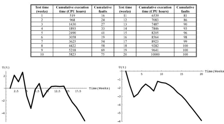
Reliability growth can be analysed by trend tests. Blindly ap-plying SRGM may not lead to meaningful results when the trend indicated by the data differs from that predicted by the model. If the model is applied to the software failure data, and shows a trend in accordance with its assumption, the results can be greatly improved [1]. Various statistical tests have been published for identifying trends in grouped data or time-series. Trend tests include graphical tests, and analytical tests. Among the analytical tests, the Laplace test is the most commonly used because it is often found to be the most appropriate one when failures & fault-removal follow NHPP [27]. Here we calculate . If the value of is negative, it indicates a decreasing failure intensity, and thus a reliability growth. On the other hand, if the value of is positive, it depicts an increasing failure intensity, and thus the reliability decreases [1], [28], [29].

For example, with reference to the above two data sets, the Laplace trend test results are shown in Figs. 1 and 2 for DS1, and DS2, respectively. As seen from Fig. 1, we find that in about the first 75% of the time, the value of is between 2, and 2; this indicates a stable reliability. Thereafter, the value of is negative, and this means a decreasing failure intensity. Thus, in this case, our proposed models can be applied. Similarly, from Fig. 2, we can see that the value of is always negative; this means a growth in reliability.

B. Criteria for Model Comparison

In general, a model can be analysed according to its ability to reproduce the observed behavior of the software, and to predict the future behavior of the software from the observed failure

Fig. 2. Laplace trend test for the second data set.

data. The two data sets listed in Section IV-A are failure counts. The three comparison criteria are:

1) The Goodness-of-Fit Criterion.

To quantitatively compare long-term predictions, we use MSE because it provides a well-understood measure of the differences between actual, and predicted values. The MSE is defined as [4], [16], [24], [30]

(22) A smaller MSE indicates a smaller fitting error, and better performance.

After the proposed model is fitted to the actual observed data, the deviation between the observed and the fitted values is evaluated by using K-S test, or the Chi-Square test. The K-S test is generally considered to be more ef-fective compared with the Chi-Square test [31]. Therefore, we will present the results of the K-S test for each selected model. Here KD will be calculated and it is defined as the maximum vertical derivation between the plot, and the line of unit slope.

2) The Predictive Validity Criterion.

The capability of the model to predict failure behavior from present & past failure behavior is called predictive validity. This approach, which was proposed by Musa [2], can be represented by computing RE for a data set

Assuming we have observed failures by the end of test time , we employ the failure data up to time

to estimate the parameters of . Substituting the esti-mates of these parameters in the MVF yields the estimate of the number of failures by time . The estimate is compared with the actual number . The procedure is re-peated for various values of . We can check the predictive validity by plotting the relative error for different values of . Numbers closer to zero imply more accurate prediction. Positive values of error indicate overestimation; negative indicate underestimation [2].

3) The Noise Criterion. The Noise is defined as [32]

(24) Small values represent less noise in the model’s prediction behavior, indicating more smoothness.

Finally, in order to check the performance of the logistic TEF, and make a comparison with the Rayleigh TEF, here we also select some comparison criteria for our evaluations [16], [33]–[36]:

(25) (26)

(27) (28)

C. Model Performance Analysis

In this section, we present our evaluation of the performance of the proposed models when applied to DS1, and DS2.

1) DS1: Fitting a proposed model to actual data involves

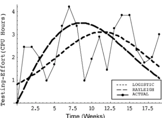
esti-mating the model parameters from the real failure data. We em-ploy the method of MLE to estimate the parameters of different SRGM. Computational details can be found in Appendix B. Similarly, all the parameters of the logistic, and Rayleigh TEF are also estimated by MLE. Firstly, the three unknown parame-ters , , and of the logistic TEF are solved by MLE, giving

the estimated values (CPU hours), , and

. Correspondingly, the estimated pa-rameters of the Rayleigh TEF are (CPU hours), and . Fig. 3 plots the comparisons between the observed failure data, and the data estimated by the logistic, and Rayleigh TEF. The PE, Bias, Variation, and MRE for the lo-gistic, and Rayleigh TEF are listed in Table III. From Table III, we see that the logistic TEF has lower values of PE, Bias,

Vari-ation, and MRE than the Rayleigh TEF. On average, the logistic

TEF yields a better fit for this data set.

Table IV lists the estimated values of parameters of different SRGM, including the Goel-Okumoto model, and the traditional

Fig. 3. Observed/estimated logistic & Rayleigh TEF for DS1.

TABLE III

COMPARISONRESULTS FORDIFFERENTTEF APPLIED TODS1

Yamada delayed S-Shaped model. We also give the values of MSE, RE, Noise, and KD in Table IV. It is observed that the SRGM with logistic TEF has the smallest value of MSE, and KD when compared with other SRGM. Because parameters of SRGM are estimated based on a limited amount of data, con-fidence estimation is necessary [2], [37]. The 90 percent confi-dence limits for all the models are given in Table V. The relevant calculation details can be found in Appendix B.

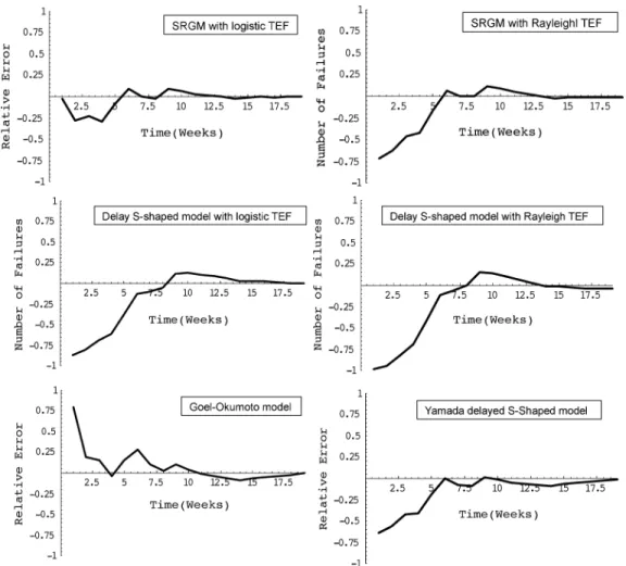
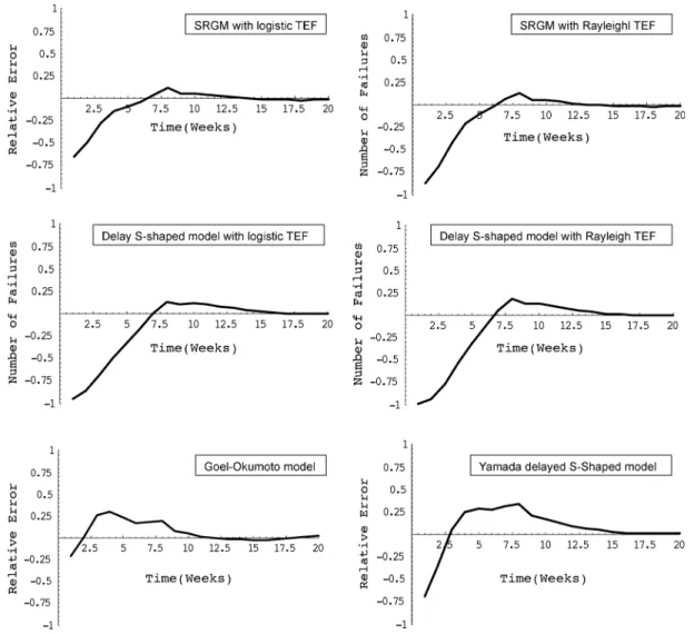
Finally, Fig. 4 depicts the RE curves for different selected models. It is worth noting that, in the study in [11], the author reported that the Yamada delayed S-shaped model may not fit the observed data well when the testing-effort spent on fault detection is not a constant. However, from Table IV, we see that the delayed S-shaped model with the logistic TEF achieves lower MSE, RE, and KD than the traditional Yamada delayed S-Shaped model, and the delayed S-Shaped model with the Rayleigh TEF. Overall, the delayed S-Shaped model with the logistic TEF predicts more accurately than these two S-shaped software reliability models.

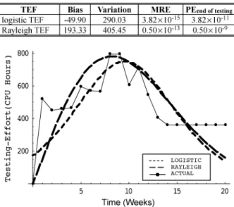
2) DS2: Similarly, the maximum likelihood estimates of the

parameters for the logistic TEF in the case of DS2 are

(CPU hours), , and .

Also, the estimated parameters for the Rayleigh TEF are

(CPU hours), and . The computed

Bias, Variation, PE, and MRE for the logistic, and Rayleigh TEF are listed in Table VI. Fig. 5 graphically illustrates the com-parisons between the observed failure data, and the data esti-mated by the logistic, and Rayleigh TEF. As seen from Fig. 5, and Table VI, similar to DS1, the logistic TEF yields a better fit than the Rayleigh TEF for DS2. Table VII shows the esti-mated values of parameters of different SRGM, and the values of MSE, RE, Noise, and KD. From Table VII, we find that the SRGM with the logistic TEF has the smallest value of MSE compared with the other SRGM. Besides, we also see that the values of MSE, and RE of the delayed S-Shaped model with the logistic TEF are still lower than those of the traditional Yamada

Fig. 4. RE curves of selected models compared with actual failure data (DS1).

TABLE IV

ESTIMATEDPARAMETERVALUES,ANDMODELCOMPARISONS FORDS1

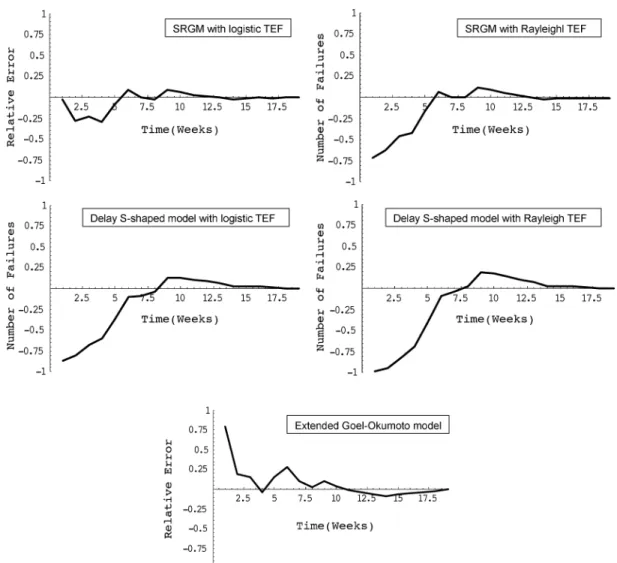
delayed S-Shaped model, and the delayed S-Shaped model with the Rayleigh TEF. The 90% confidence limits for the proposed models are also given in Table VIII. And Fig. 6 depicts the RE curves for all selected models.

Finally, software reliability depends on the pattern of oper-ation of the software, and the performance of SRGM strongly depends on the kind of data set. If the software development project managers plan to employ SRGM for estimation of re-liability growth of products during software development pro-cesses, the software developers or reliability engineers need to select several representative models, and apply them in parallel. Although models sometimes give good results, there is no single model that can be trusted to give accurate results in all circum-stances, nor is there a way in which the most suitable model can

be chosen a priori for a particular situation [1], [3], [4]. From our results, we can conclude that the logistic TEF may be a good approach to providing a more accurate description of resource consumption during the software development phase than pre-vious approaches. By incorporating the logistic TEF into both exponential-type, and S-shaped software reliability models, the modified SRGM become more powerful, and more informative in the software reliability engineering process.

V. IMPERFECTDEBUGGINGMODELING

In general, different SRGM make different assumptions, and therefore can be applied to different situations. Most SRGM published in the literature assume that each time a failure oc-curs, the fault that caused it is immediately removed, and no

TABLE V

90% CONFIDENCELIMITS FORDIFFERENTSELECTEDMODELS(DS1)

TABLE VI

COMPARISONRESULTS FORDIFFERENTTEF APPLIED TODS2

Fig. 5. Observed/estimated logistic & Rayleigh TEF for DS2.

new faults are introduced. Besides, some people also assume that the correction of a fault takes only negligible time, and the detected fault is removed with certainty [38]–[40]. These assumptions help to reduce the complexity of modeling soft-ware reliability growth; however, in reality, developers experi-ence cases where they fix one bug, but create another new one. Debugging is in fact a complex cognitive activity because it con-sists of locating & correcting the faults that generated the ob-served failures. Therefore, imperfect debugging could occur in the real world.

There are many papers that have addressed the problem of im-perfect debugging [40]–[48]. For instance, Ohba & Chou [44] reported that, in their study, about 14 percent of the faults de-tected & removed during an observation period would intro-duce new faults as a result of imperfect debugging. They also demonstrated that, in such cases, SRGM are still applicable, al-though imperfect debugging caused some variation in the pa-rameter values of the engaged models. On the other hand, Goel & Okumoto [48] showed that an imperfect debugging model provided a good fit to the software failure data from a real-time control system for a land-based radar system developed by the Raytheon Company. Xie & Yang [41] tried to investigate the effect of imperfect debugging on software development costs. They extended a commonly used cost model to the case of im-perfect debugging. In addition, Zhang et al. [45] also proposed

a method to integrate fault removal efficiency, and fault intro-duction rate into SRGM. Therefore, we have to consider the imperfect debugging problem when we propose a new SRGM, as it provides an essential, valuable insight into the debugging process.

In this section, we investigate a relaxation of the perfect de-bugging assumption. We modify the assumption 6 presented in Section III-A to be as follows: When a fault is detected &

re-moved, new faults may be generated. Besides, when removing or fixing a detected fault, the probability of introducing another

fault is a constant . Based on assumptions 1–5 described in

Section III-A, we can describe in detail the SRGM with the logistic TEF within an imperfect debugging environment. Ac-cording to these assumptions, we rewrite (7) as

(29) Note that is generally defined as the sum of the expected number of initial software faults, and introduced faults as a func-tion of time [4], [45].

Mathematically, assuming that

(30) solving (29) by substituting (30) into it, and assuming

& , we obtain the MVF

(31) We also have

(32) It is noted that is given by

(33) In this case, we have

(34) Similarly, we can modify the assumption 8 presented in Sec-tion III-B. For example, by using (19), we have

Fig. 6. RE curves of selected models compared to actual failure data (DS2).

TABLE VII

ESTIMATEDPARAMETERVALUES,ANDMODELCOMPARISONS FORDS2

Solving (35) under the boundary condition , the layed S-Shaped model with logistic TEF under imperfect de-bugging is given by

(36) These above equations (31) & (36) can represent the case where a fault is not successfully removed, and new faults are intro-duced during the testing/debugging phase.

Due to the space limitations, here we use only DS1 (i.e., the Ohba data) to discuss the issue of imperfect debugging.

Simi-larly, the parameters , , and in (31), and (36) can be solved numerically by the method of MLE. Moreover, as discussed in [44], we can apply the extended Goel-Okumoto model by taking account of imperfect debugging with MLE for param-eter estimation. Table IX gives the estimated paramparam-eters of se-lected models under imperfect debugging, and results of model comparisons. It is observed that the values of MSE and KD of the SRGM with the logistic TEF are the lowest among all the models considered. Besides, we also see that the values of MSE, RE, Noise, and KD of the delayed S-Shaped model with the lo-gistic TEF are still lower than those of the delayed S-Shaped model with Rayleigh TEF.

TABLE VIII

COMPARISONS OF90% CONFIDENCELIMITS FORDIFFERENTSELECTEDMODELS(DS2)

TABLE IX

ESTIMATEDPARAMETERVALUES,ANDMODELCOMPARISONSUNDERIMPERFECTDEBUGGING(DS1)

TABLE X

90% CONFIDENCELIMITS FORSRGM UNDERIMPERFECTDEBUGGING(DS1)

From Table IX, we observe that the fault removal process in the software development & testing environment may not be a pure perfect debugging process because the estimated values of are all close but not equal to zero. For example, we can see that the fault introduction rate of the SRGM with the logistic TEF is . This means that, on the average, one fault will be introduced per about 100 removed faults. Hence, we see that the introduction of new faults during the correction process tends to be a minor effect in the development process if we apply the software reliability models listed in Table IX. Actually, Yin et

al. [43] reported that, from a statistical point of view, the number

of introduced faults is less significant when the total number of remaining faults is relatively large. They postulated that the im-perfect debugging should be taken into account when the soft-ware product is reaching the mature stage, where the number of remaining faults, and the number of introduced faults are of the same order of magnitude [43], [49]. In addition to (30), there may be other useful fault content functions [24], [45], but fur-ther discussion of this topic is beyond the scope of this paper. The 90% confidence limits for the selected models are given in Table X, while Fig. 7 illustrates the RE curves for different models. Altogether, these metrics can provide engineers with in-sightful information about software development & testing ef-forts, and help project managers make the best decisions in al-locating testing resources.

APPENDIXA

From (16), we note that, if is approximately the same as , the right hand side of this equation will approach negative infinity. In this case, we let

(37) and

(38) From L’Hospital’s Rule, we know

Fig. 7. RE curves of selected models under imperfect debugging compared to actual failure data (DS1). Thus, we obtain (40) and (41) That is, (42) Therefore, (43) APPENDIXB

Fitting a proposed model to actual fault data involves esti-mating the model parameters from the real test data sets. Here

we employ the method of MLE to estimate the parameters , and [1], [2]. All parameters of different TEF can be estimated by the method of MLE. For example, suppose that , and are determined for the observed data pairs:

Then the likelihood function for the parameters , and in the NHPP model with in (9) is given by

(44)

where for .

Taking the natural logarithm of the likelihood function in (44), we have

From (9), we know that

. Thus,

(46) Consequently, the maximum likelihood estimates of , and can be obtained by solving

(47) Therefore, we obtain

(48) and (49) at the bottom of the page. Therefore, , and can be solved by numerical methods.

Similarly, for the delayed S-Shaped model with logistic TEF, we can get

(50) and (51) at the bottom of the page.

Finally, if the sample size of is sufficiently large, then the maximum-likelihood estimates , and of the SRGM’s parameters , and asymptotically follow a bivariate -normal (BVN) distribution [13], [15], [16], [22]

(52)

The mean values of , and are the true values of , and , re-spectively; and the variance-covariance matrix is given by the inverse matrix of the Fisher information matrix [50]. The Fisher information matrix for the two-parameter NHPP model (i.e.,

, and ) can be derived from as

(53)

Applying , and to the above equation, and calculating , the large sample asymptotic variance-covariance matrix is given by

(54) The variance-covariance matrix is useful in quantifying the variability of the estimated parameters. The two-sided approxi-mate confidence limits for , and can then be obtained in a standard way [13], [37], [50]. For example, the two-sided approximate 100\alpha% confidence limits for the parameters

, and are (55) (56) (57) and (58) where is the quartile of the standard -normal distribution.

ACKNOWLEDGMENT

The authors would like to thank Editor Prof. M. A. Vouk for his constructive, insightful suggestions, which led to a signifi-cant improvement of this paper.

(49)

REFERENCES

[1] M. R. Lyu, Handbook of Software Reliability Engineering. : McGraw Hill, 1996.

[2] J. D. Musa, A. Iannino, and K. Okumoto, Software Reliability,

Mea-surement, Prediction and Application. : McGraw Hill, 1987. [3] S. S. Gokhale and M. R. Lyu, “A simulation approach to

struc-ture-based software reliability analysis,” IEEE Trans. Software

Engineering, vol. 31, no. 8, pp. 643–656, August 2005.

[4] M. Xie, Software Reliability Modeling. : World Scientific Publishing Company, 1991.

[5] A. T. Rivers, “Modeling Software Reliability During Non-Operational Testing,” Ph.D. Dissertation, Department of Computer Science, North Carolina State University, Raleigh, NC, 1998.

[6] S. S. Gokhale and K. S. Trivedi, “Log-logistic software reliability growth model,” in Proceedings of the 3rd IEEE International

High-As-surance Systems Engineering Symposium (HASE ’98), Washington,

DC, USA, Nov. 1998, pp. 34–41.

[7] Y. Tamura and S. Yamada, “Comparison of software reliability assess-ment methods for open source software,” in Proceedings of the 11th

In-ternational Conference on Parallel and Distributed Systems (ICPADS 2005), Los Almitos, CA, USA, July 2005, pp. 488–492, IEEE

Com-puter Society.

[8] C. Y. Huang, M. R. Lyu, and S. Y. Kuo, “A unified scheme of some non-homogenous Poisson process models for software reliability estimation,” IEEE Trans. Software Engineering, vol. 29, no. 3, pp. 261–269, March 2003.

[9] A. Gana and S. T. Huang, “Statistical modeling applied to managing global 5ess- 2000 switch software development,” Bell Labs Technical

Journal, vol. 2, no. 1, pp. 144–153, Winter 1997.

[10] G. A. Kruger, “Validation and further application of software reliability growth models,” Hewlett-Packard Journal, vol. 40, no. 4, pp. 75–79, April 1989.

[11] M. Ohba, “Software reliability analysis models,” IBM Journal of

Re-search and Development, vol. 28, no. 4, pp. 428–443, 1984.

[12] S. H. Kan, Metrics and Models in Software Quality Engineering, 2nd ed. : Addison-Wesley, 2003.

[13] S. Yamada, J. Hishitani, and S. Osaki, “Software reliability growth model with Weibull testing effort: a model and application,” IEEE

Trans. Reliability, vol. R-42, pp. 100–105, 1993.

[14] M. U. Bokhari and N. Ahmad, “Analysis of a software reliability growth models: The case of log-logistic test-effort function,” in

Pro-ceedings of the 17th IASTED International Conference on Modelling and Simulation (MS 2006), Montreal, Quebec, Canada, May 2006, pp.

540–545.

[15] P. K. Kapur, D. N. Goswami, and A. Gupta, “A software reliability growth model with testing effort dependent learning function for distributed systems,” International Journal of Reliability, Quality and

Safety Engineering, vol. 11, no. 4, pp. 365–377, 2004.

[16] C. Y. Huang and S. Y. Kuo, “Analysis and assessment of incorporating logistic testing effort function into software reliability modeling,” IEEE

Trans. Reliability, vol. 51, no. 3, pp. 261–270, Sept. 2002.

[17] S. Y. Kuo, C. Y. Huang, and M. R. Lyu, “Framework for modeling soft-ware reliability, using various testing-efforts and fault-detection rates,”

IEEE Trans. Reliability, vol. 50, no. 3, pp. 310–320, Sept. 2001.

[18] C. Y. Huang, S. Y. Kuo, and M. R. Lyu, “Effort-index-based software reliability growth models and performance assessment,” in

Proceed-ings of the 24th Annual International Computer Software and Applica-tions Conference (COMPSAC 2000), Taipei, Taiwan, Oct. 25–27, 2000,

pp. 454–459.

[19] B. Boehm, Software Engineering Economics. : Prentice-Hall, 1981. [20] K. Pillai and V. S. Sukumaran Nair, “A model for software

develop-ment effort and cost estimation,” IEEE Trans. Software Engineering, vol. 23, no. 8, pp. 485–497, Aug. 1997.

[21] T. DeMarco, Controlling Software Projects: Management,

Measure-ment and Estimation. Englewood Cliffs, NJ: Prentice-Hall, 1982. [22] P. K. Kapur, R. B. Garg, and S. Kumar, Contributions to Hardware and

Software Reliability. : World Scientific Publishing Company, 1999. [23] F. N. Parr, “An alternative to the Rayleigh curve for software

devel-opment effort,” IEEE Trans. Software Engineering, vol. SE-6, pp. 291–296, 1980.

[24] H. Pham, Software Reliability. : Springer-Verlag, 2000.

[25] S. Yamada, M. Ohba, and S. Osaki, “S-shaped software reliability growth models and their applications,” IEEE Trans. Reliability, vol. R-33, no. 4, pp. 289–292, Oct. 1984.

[26] A. P. Wood, “Predicting software reliability,” IEEE Computer, pp. 69–77, Nov. 1996.

[27] A. L. Goel and K. Z. Yang, “Software reliability and readiness assess-ment based on the non-homogeneous Poisson process,” Advances in

Computers, vol. 45, pp. 197–267, 1997.

[28] K. Kanoun and J. C. Laprie, “Software reliability trend analyses from theoretical to practical considerations,” IEEE Trans. Software

Engi-neering, vol. 20, no. 9, pp. 740–747, 1994.

[29] K. Kanoun, M. Kaaniche, and J. C. Laprie, “Qualitative and quantita-tive reliability assessment,” IEEE Software, vol. 14, no. 2, pp. 77–87, March–April 1997.

[30] P. K. Kapur and S. Younes, “Software reliability growth model with error dependency,” Microelectronics and Reliability, vol. 35, no. 2, pp. 273–278, 1995.

[31] Y. K. Malaiya, N. Karunanithi, and P. Verma, “Predictability measures for software reliability models,” in Proceedings of the 14th IEEE

An-nual International Computer Software and Applications Conference (COMPSAC’90), Chicago, Illinois, USA, Oct. 7–12, 1990.

[32] M. R. Lyu and A. Nikora, “Using software reliability models more ef-fectively,” IEEE Software, pp. 43–52, July 1992.

[33] M. Shepperd and C. Schofield, “Estimating software project effort using analogies,” IEEE Trans. Software Engineering, vol. 23, pp. 736–743, 1997.

[34] K. Srinivasan and D. Fisher, “Machine learning approaches to estimating software development effort,” IEEE Trans. Software

Engi-neering, vol. 21, no. 2, pp. 126–136, 1995.

[35] K. Pillai and V. S. Sukumaran Nair, “A model for software develop-ment effort and cost estimation,” IEEE Trans. Software Engineering, vol. 23, no. 8, August 1997.

[36] K. Srinivasan and D. Fisher, “Machine learning approaches to estimating software development effort,” IEEE Trans. Software

Engi-neering, vol. 21, no. 2, pp. 126–136, 1995.

[37] M. Xie, “Software reliability models—Past, present and future,” in

Re-cent Advances in Reliability Theory: Methodology, Practice and Infer-ence, N. Limnios and M. Nikulin, Eds. Boston: Birkhauser, 2000, pp. 323–340.

[38] N. F. Schneidewind, “Fault correction profiles,” in Proceedings of

the 14th IEEE International Symposium on Software Reliability Engineering (ISSRE 2003), Denver, Colorado, USA, Nov. 2003, pp.

257–267.

[39] K. Goˇseva-Popstojanova and K. S. Trivedi, “Failure correlation in soft-ware reliability models,” IEEE Trans. Reliability, vol. 49, no. 1, pp. 37–48, March 2000.

[40] J. H. Lo and C. Y. Huang, “Incorporating imperfect debugging into software fault correction process,” in Proceedings of the IEEE Region

10 Annual International Conference (TENCON 2004), Chiang Mai,

Thailand, Nov. 2004, pp. 326–329.

[41] M. Xie and B. Yang, “A study of the effect of imperfect debugging on software development cost,” IEEE Trans. Software Engineering, vol. 29, no. 5, pp. 471–473, May 2003.

[42] P. E. Ammann, S. S. Brilliant, and J. C. Knight, “The effect of imperfect error detection on reliability assessment via life testing,” IEEE Trans. Software Engineering, vol. 20, no. 2, pp. 142–148, Feb. 1994.

[43] M. L. Yin, L. E. James, S. Keene, R. R. Arellano, and J. Peterson, “An adaptive software reliability prediction approach,” in The 23rd Annual

Software Engineering Workshop, Greenbelt, Maryland, Dec. 1998

[Online]. Available: http://sel.gsfc.nasa.gov/website/sew/1998/pro-gram.htm

[44] M. Ohba and X. Chou, “Does imperfect debugging affect software re-liability growth?,” in Proceedings of the 11th International Conference

on Software Engineering (ICSE’89), Pittsburgh, USA, May 1989, pp.

237–244.

[45] X. Zhang, X. Teng, and H. Pham, “Considering fault removal efficiency in software reliability assessment,” IEEE Trans. Systems, Man, and

Cy-bernetics—Part A: Systems and Humans, vol. 33, no. 1, pp. 2241–2252,

Jan. 2003, 114-120.

[46] S. Yamada, K. Tokuno, and S. Osaki, “Imperfect debugging models with fault introduction rate for software reliability assessment,”

Inter-national Journal of Systems Science, vol. 23, no. 12, pp. 2241–2252,

1992.

[47] W. Bodhisuwan and P. Zeephongsekul, “Asymptotic properties of a statistical model in software reliability with imperfect debugging and introduction of defects,” in Proceedings of the 9th ISSAT International

Conference on Reliability and Quality in Design, Honolulu, Hawaii,

August 2003.

[48] A. L. Goel and K. Okumoto, “An analysis of recurrent software errors in a real-time control system,” in Proceedings of the 1978 Annual

[49] M. C. J. van Pul, “Statistical Analysis of Software Reliability Models,” PhD. Dissertation, Department of Mathematics, Utrecht University, , Netherlands, 1993.

[50] W. Nelson, Applied Life Data Analysis. New York: Wiley, 1982. Chin-Yu Huang is currently an Assistant Professor in the Department of Com-puter Science at National Tsing Hua University, Hsinchu, Taiwan. He received the MS (1994), and the Ph.D. (2000) in Electrical Engineering from National Taiwan University, Taipei. He was with the Bank of Taiwan from 1994 to 1999, and was a senior software engineer at Taiwan Semiconductor Manufacturing Company from 1999 to 2000. Before joining National Tsing Hua University in 2003, he was a division chief of the Central Bank of China, Taipei, Taiwan. His research interests are in software reliability engineering, fault tree analysis, software testing, and testability. He is a member of IEEE.

Sy-Yen Kuo is Dean of the College of Electrical and Computer Engineering, Na-tional Taiwan University of Science and Technology, Taipei, Taiwan. He is also a Professor at the Department of Electrical Engineering, National Taiwan Uni-versity where he is currently on leave, and was the Chairman at the same depart-ment from 2001 to 2004. He received the BS (1979) in Electrical Engineering from National Taiwan University, the MS (1982) in Electrical & Computer En-gineering from the University of California at Santa Barbara, and the Ph.D. (1987) in Computer Science from the University of Illinois at Urbana-Cham-paign. He spent his sabbatical years as a Visiting Professor at the Computer Science and Engineering Department at the Chinese University of Hong Kong from 2004–2005, and as a visiting researcher at AT&T Labs-Research, New Jersey from 1999 to 2000, respectively. He was the Chairman of the Depart-ment of Computer Science and Information Engineering, National Dong Hwa University, Taiwan from 1995 to 1998, a faculty member in the Department of Electrical and Computer Engineering at the University of Arizona from 1988 to 1991, and an engineer at Fairchild Semiconductor and Silvar-Lisco, both in Cali-fornia, from 1982 to 1984. In 1989, he also worked as a summer faculty fellow at the Jet Propulsion Laboratory of the California Institute of Technology. His cur-rent research interests include dependable systems and networks, software reli-ability engineering, mobile computing, and reliable sensor networks. Professor Kuo is an IEEE Fellow. He has published more than 260 papers in journals, and conferences. He received the distinguished research award between 1997 and 2005 consecutively from the National Science Council in Taiwan, and is now a

Research Fellow there. He was also a recipient of the Best Paper Award in the 1996 International Symposium on Software Reliability Engineering, the Best Paper Award in the simulation and test category at the 1986 IEEE/ACM Design Automation Conference (DAC), the National Science Foundation’s Research Initiation Award in 1989, and the IEEE/ACM Design Automation Scholarship in 1990 and 1991.

Michael R. Lyu is currently a Professor in the Department of Computer Science and Engineering, the Chinese University of Hong Kong. He is also Director of the Video over InternEt and Wireless (VIEW) Technologies Laboratory. He re-ceived the BS (1981) in Electrical Engineering from National Taiwan Univer-sity, the MS (1982) in Electrical & Computer Engineering from the University of California at Santa Barbara, and the Ph.D. (1988) in Computer Science from the University of California, Los Angeles. He was with the Jet Propulsion Labora-tory as a Technical Staff Member from 1988 to 1990. From 1990 to 1992, he was with the Department of Electrical and Computer Engineering at the University of Iowa as an Assistant Professor. From 1992 to 1995, he was a Member of the Technical Staff in the applied research area of Bell Communications Research (Bellcore), Morristown, New Jersey. From 1995 to 1997, he was a Research Member of the Technical Staff at Bell Laboratories, Murray Hill, New Jersey. His research interests include software reliability engineering, distributed sys-tems, fault-tolerant computing, mobile networks, Web technologies, multimedia information processing, and E-commerce systems. He has published over 250 refereed journal and conference papers in these areas. He received Best Paper Awards in ISSRE’98, and ISSRE’2003. He was the editor of two book vol-umes: Software Fault Tolerance (New York: Wiley, 1995), and The Handbook of Software Reliability Engineering (Piscataway, NJ: IEEE and New York: Mc-Graw-Hill, 1996). Dr. Lyu initiated the First International Symposium on Soft-ware Reliability Engineering (ISSRE) in 1990. He was the Program Chair for ISSRE’96, and General Chair for ISSRE’2001. He was also PRDC’99 Program Co-Chair, WWW10 Program Co-Chair, SRDS’2005 Program Co-Chair, and PRDC’2005 General Co-Chair, and served in program committees for many other conferences. He served on the Editorial Board of IEEE TRANSACTIONS ONKNOWLEDGE ANDDATAENGINEERING, and has been an Associate Editor of IEEE TRANSACTIONS ONRELIABILITY, Journal of Information Science and En-gineering, and Wiley Software Testing, Verification & Reliability Journal. Dr. Lyu is an IEEE Fellow, and an AAAS Fellow, for his contributions to software reliability engineering, and software fault tolerance.