Interpretation of Temperature Control for Ternary Distillation

(1)

Industrial & Engineering Chemistry Research is published by the American Chemical Society. 1155 Sixteenth Street N.W., Washington, DC 20036

Article

Interpretation of Temperature Control for Ternary Distillation

Min-Te Lin, Cheng-Ching Yu, and Michael L. Luyben

Ind. Eng. Chem. Res., 2005, 44 (22), 8277-8290 • DOI: 10.1021/ie050130m

Downloaded from http://pubs.acs.org on November 28, 2008

Interpretation of Temperature Control for Ternary Distillation

Min-Te Lin,†_{Cheng-Ching Yu,*},†_{and Michael L. Luyben}‡

Department of Chemical Engineering, National Taiwan University, Taipei 106-17, Taiwan, and E. I. du Pont de Nemours & Co., Inc., 1007 Market St. - B7434, Wilmington, Delaware 19898

Even with recent advances in technology for on-line composition measurement, temperature remains the dominant control configuration in distillation columns for product purity. In controlling industrial ternary distillation columns, with a nonmonotonic composition profile for the intermediate boiler, significantly different closed-loop composition dynamics are observed when the temperature-control tray is above or below the intermediate boiler composition turning point (i.e., above or below the tray where the intermediate exhibits a maximum). In this work, the role of direct temperature control is interpreted in the composition space. First, the temperature isotherm is established in the triangular composition space and the process direction and control direction can be clearly distinguished. Then, a quantitative measure, called the traveling distance, for all tray compositions under a specific temperature-control configuration is defined. The traveling distance can be computed directly from process and load transfer function matrices. Rigorous nonlinear distillation column simulations confirm that a temperature-control point with a large traveling distance results in slow composition dynamics (e.g., considering the tray composition can be changed with a fixed rate) and, consequently, poorer control performance. The situation with the difference in traveling distance can become worse when two temperatures are controlled in the column. Finally, this concept is extended to direct composition control of ternary distillation systems. The results clearly show that improved temperature or composition control can be achieved by avoiding a potential conflict in the process and control directions.

1. Introduction

Distillation remains the dominant separation technol-ogy in many industrial processes. The control of distil-lation columns has been the subject of much work over the decades that continues today as new problems and challenges emerge. For simple column configurations (one feed, no intermediate heat sources or sinks, and two product streams), we have six degrees of freedom available for manipulation (feed flow, reboiler duty, bottoms flow, condenser duty, reflux flow, and distillate flow). We also have three inventory variables that must be controlled within some range (pressure, reflux drum level, and base level). Feed flow is typically set by the unit upstream of the column. This leaves two degrees of freedom available for controlling column product composition.

The design basis for columns typically involves speci-fying certain purities or component recoveries in one or two product streams. The achievement of the design objectives depends on the performance of the column controls. In principle, we would like to have direct, instantaneous on-line measurement of product purities. Many advances have been made in technology for on-line composition measurement. But we still have many systems where such measurements do not exist, are too hazardous, are not feasible, are not maintained ad-equately, are too slow, are too expensive, etc. Hence,

column temperatures are still the main controlled variable in distillation columns for product purity control.

Temperature control of distillation columns has been the subject of numerous papers over the last 50 years.

Rademaker et al.1 _{present a good summary of the}

various ideas and criteria generated over the years. Buckley et al.2_{discuss various approaches for indirect} composition control, which include differential temper-ature, pressure-compensated tempertemper-ature, double-dif-ferential temperature, and average temperature. Most of the temperature selection criteria are based on the sensitivity with respect to input or load changes. Downs and Moore3_{propose a multivariable version using the} singular value decomposition (SVD). Following in the same vein, the nonsquare relative gain (NRG) by Chang and Yu4 _{and Cao and Rossiter}5 _{is also effective in} screening possible temperature-control trays. Another approach to indirect composition control is to estimate composition from temperature measurements. This work includes heuristic-based modeling,6 least-squares-based modeling,7 _{and partial least-squares-based} modeling.8-11 _{The above-mentioned approaches may} provide effective temperature control, but the explana-tion behind the success or failure of different temper-ature-control points is rarely addressed, particularly for multicomponent systems.

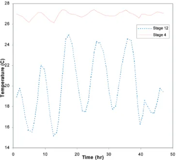
The motivation for this work comes from experience on an actual industrial distillation column.12 _This column effectively separates 3 components and has∼32 theoretical stages with the temperature profile shown in Figure 1. When we choose a temperature-control * Corresponding author. Tel.: 2-3365-1759. Fax:

+886-2-3366-3037. E-mail: [email protected].

†_{National Taiwan University.} ‡_{E. I. du Pont de Nemours & Co., Inc.}

8277 Ind. Eng. Chem. Res. 2005, 44, 8277-8290

(3)

location, we typically look for a point where the tem-perature changes significantly over a few trays. This tends to indicate a break in the composition profile of a component and means that the temperature will be sensitive to a manipulator (e.g., reflux flow or reboiler duty). We do not want to choose a temperature that is in a flat zone, since it will not be sensitive to changes in column conditions.

In the industrial column, theoretical stage 4 (from bottom) was historically used for decades as the tem-perature-control location with reboiler steam flow as the manipulator. This seems to be a reasonable choice when looking at the temperature profile. However, whenever the column experienced a significant change in the feed composition of the intermediate component, the tem-peratures above stage 4 would undergo cycles of much greater magnitude than what was seen on stage 4. Figure 2 shows some actual column data where stage 4 temperature is being controlled within∼1 °C while the stage 12 temperature cycles by over 4 °C. A study on this column showed that this behavior arose from the

composition profile of the intermediate-boiling compo-nent and that it mattered whether the temperature-control location is chosen above or below the tray where the intermediate boiler exhibits a maximum.

This paper studies the problem of temperature control for a generic ternary distillation column. We focus on a ternary mixture since multicomponent columns can often be simplified down to three-component systems. We interpret the temperature profile in composition space and define a quantitative measure, called the traveling distance, to explain why we want to select a temperature-control location on the correct side of the intermediate-boiling component profile maximum. 2. Interaction between Temperature and Composition

2.1. Process Description. We consider as an ex-ample a three-component (A, B, and C) separation assuming the following constant relative volatilities:

Figure 3 shows in triangular composition space the direct separation process where component A is removed overhead and components B and C are removed in the bottoms. Table 1 contains the steady-state column process conditions for a design with 25 theoretical stages. We have assumed certain vapor pressure coef-ficients in an Antoine-type correlation to translate from Figure 1. Industrial column temperature profile.

Figure 2. Cycling in column temperatures.

Figure 3. Triangular composition space for direct separation with

material balance line.

Table 1. Steady-State Operating Conditions

column feed flow rate (F) 100.0 (lbmol/h) reflux flow rate (R) 109.222 (lbmol/h) distillate flow rate (D) 50.848 (lbmol/h) reflux ratio (RR) 2.148 (mole fraction) bottom flow rate (B) 49.152 (lbmol/h) vapor boilup (V) 160.169 (lbmol/h) no. of trays (NT) 25

feed tray (NF) 18

relative volatilities (RA/RB/RC) 4/2/1

hydraulic time constant (β) 3.2 (s) bottom holdup (MB) 17.435 (lbmol)

reflux holdup (MD) 13.339 (lbmol)

tray holdup (MN) 0.592 (lbmol)

feed composition (ZA/ZB/ZC) 0.5/0.2564/0.2436 (mole frac)

distillate composition (xD,A/xD,B/xD,C) 0.982/1.75E-2/5E-4

(mole frac)

bottom composition (xB,A/xB,B/xB,C) 0.001/0.503/0.496 (mole frac)

Antoine vapor pressure coefficient (AA/AB/AC/B)

15.2/14.51/13.8/-2768.55 normal boiling point (TA, TB, TC) 323.15, 351.6, 385.54 (K)

R

(4)

the composition space to a temperature profile. Figure 4 shows the composition and temperature profiles for the column. The key feature to note is the behavior of the intermediate boiler (component B). As we go down the column, the composition of B increases until we

reach a maximum of ∼0.8 mole fraction at about

theoretical stage 5; then the composition decreases and is only 0.5 mole fraction in the bottoms product. This nonmonotonic composition profile exists in all ternary distillation columns, making them unique from binary separations, for both ideal and nonideal components. Where we want to choose the temperature-control point is governed by the location of this maximum. For the ideal distillation system with the equal molar overflow assumption, the relationship between temperature and composition can be described by the bubble point temperature equation:

Note that the Antoine coefficient B is constant for the ideal system. P is the column pressure, and T is temperature. Rearranging the equation, the tempera-ture can be obtained directly given the liquid-phase composition.

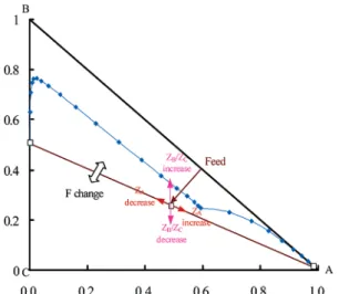
2.2. Temperature Control and Observations. If we consider typical load disturbances for the column,

we can visualize how they affect the column in composi-tion space (Figure 5). Changes in the feed composicomposi-tion of A, ZA, will move along the direction of the straight line connecting the distillate and bottoms compositions. Changes in the ratio of the feed compositions of B and C, ZB/ZC, will move the process along a vertical direc-tion. Changes in the feed flow will either stretch/ compress the end points of the material balance line or rotate the material balance line using the feed point as the origin or pivot. The particular open-loop behavior depends on the chosen control structure (e.g., fixing reflux-vapor rate or distillate-vapor rate).

A standard dual-composition control strategy is shown in Figure 6. We use reflux to control a temperature toward the top of the column and reboiler duty to control a temperature toward the bottom of the column. This is called the R-V strategy. Many columns operate with Figure 4. Composition and temperature profile for the system

T ) B ln P

xAexp(AA) + xBexp(AB) + xCexp(AC)

Figure 5. Nominal column composition profile, material balance

line, and effects of load disturbances on the feed location (ZAand ZB/ZCchanges) and material balance line (F change).

Figure 6. Dual-end temperature control with R-V control

structure.

(5)

only single-end control that uses one temperature. Since vapor boilup has a fast and significant effect on column temperatures, it often is the manipulator of choice. We need to determine which temperature to use for control. The two common requirements in picking a good tem-perature-control location are (1) we want the manipula-tor to have a significant effect on the temperature (ratio

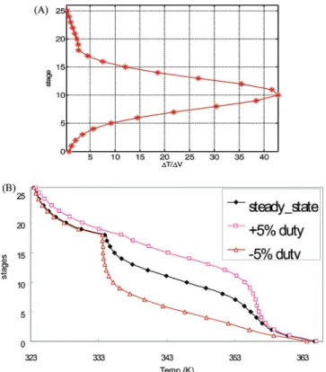
of temperature change to manipulator change is large) and (2) we want the response to be somewhat symmetric (an increase or decrease in manipulator causes about the same relative effect). Figure 7A shows the sensitivity analysis of the temperature profile to a 0.001% change in vapor boilup. If we look at possible temperature-control trays, T1 is somewhat related to the bottoms-product composition but it does not have a large gain,

T5is the tray location giving the maximum in compo-nent B composition xj,B,max, and T10is the most sensitive tray. Vapor boilup changes of (5% indicate that T10has a quite symmetric response, as shown in Figure 7b.

We now compare the temperature response of these three possible control-tray locations using a rigorous, nonlinear dynamic simulation of the column.13_{For a} given control structure, decentralized PI controllers are tuned automatically. First, the ultimate gain and ulti-mate period are identified using sequential relay feed-back as presented by Shen and Yu.14 _{Then, the PI} controller settings are obtained following the Tyreus and Luyben15 _{tuning rule. Figure 8 shows a (10% Z}

B/ZC change. What we can observe is that the temperature dynamics give somewhat comparable speeds of response. However, when we use a temperature-control tray below the maximum xi,B,max, we get much more sluggish

composition dynamics. Similar behavior is observed for feed flow rate and ZAchanges.

2.3. Isotherms in Composition Space. To explain more quantitatively what we observe with the closed-loop simulations, we can look at temperature isotherms in composition space (since we are controlling temper-ature in the column as a proxy for composition). From vapor-liquid equilibrium (VLE), we have

where yiand xiare the mole fractions in the vapor and

Figure 7. (A) Temperature sensitivity for (0.001% change in

boilup rate and (B) temperature profile for (5% change in boilup rate.

Figure 8. Closed-loop responses with different temperature-control trays (T1, T5, and T10control) for (10% ZB/ZCchanges.

(6)

liquid phases, P is the total pressure, and P_isat is the vapor pressure of the pure components. We know that

the sum of the vapor mole fractions and the total pressure must satisfy

From the Clausius-Clapeyron equation, we can relate the vapor pressure to temperature via a reference temperature and vapor pressure.

where ∆Hiis the molar heat of vaporization and R is

the gas constant. At low pressure with constant relative volatilities

Figure 9. Constant temperature line in the composition space.

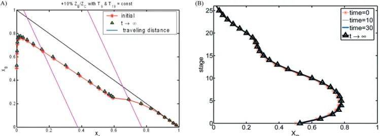
Figure 10. Reshaping composition profile for -20% F change with (A) T1control, (B) T5control, and (C) T10control for: (top) initial and

final composition profiles with traveling distance (shown by arrow), (middle) evolution of composition profile of B, and (bottom) snapshots of composition profile of B as time approaches 0, 10, 30, and∞.

∑

y_i) 1 ) Σ xiPi sat P (2) P ) Σx_iP_isat (3) Pi sat_{) P} i,0exp

[

-∆Hi R

(

1 T- 1T₀

)

]

(4) Ind. Eng. Chem. Res., Vol. 44, No. 22, 2005 8281

(7)

where Kiis the K-value of the ith component.

Equal molar overflow assumes ∆Hi is constant over

the temperature range of interest for all components, ∆Hi) ∆H. We can obtain

If we let the heavy component C be the reference component (xA) xB) 0 and xC) 1 with RC) 1), we get (∑xiRi)0) ((0 × 4) + (0 × 2) + (1 × 1)) ) 1. After some rearrangement, we have

where T_Csat is the boiling-point temperature of compo-nent C at the given pressure. Finally, we get

and

This is an equation for a straight line in xA- xBspace with a slope and intercept for temperature isotherm lines. The slope is -(RA- 1)/(RB- 1) and the intercept can be expressed as (1/(RB - 1)) {exp[(∆H/R)((1/T) -(1/T_Csat))] - 1}. This is shown in Figure 9. So when we use a temperature for control with a constant setpoint, the direction of movement is along this iso-therm line.

2.4. Analysis. Figure 10 shows what happens to the column composition profile for a 20% decrease in feed flow with the three different constant temperature-control trays. With constant T1 (the temperature has to lie on the temperature isotherm), the column com-position profile has to change much more than with constant T10, as shown in the first row of Figure 10. Despite the fact that the final column composition profiles almost coincide with the initial one for all three cases, the tray composition is very different from the nominal one when T1is kept constant. The 3-D plots in the second row of Figure 10 reveal that the column takes a longer time to settle if the tray composition travels a significant distance in the composition space. The snapshots of the composition profile of component B at times (in min) approaching 0, 10, 30, and∞show very different speeds of response for T1, T5, and T10control. The following observations can be made immediately. First, under a load change, the entire column composi-tion profile covered by the column does not change much, at least visually. Second, the internal (tray) compositions may be very different using different

temperature-control trays. Third, the distance each tray composition travels (in the composition space) is associ-ated with the speed of response. Similar behavior is also observed for ZAand ZB/ZCdisturbances.

]

) (RA- 1)xA+ (RB- 1)xB+ 1 xB) -(RA- 1) (RB- 1) x_A+ 1 (RB- 1)

{

exp

[

∆H vap R

(

1 T- 1_T C sat

)

]

- 1

}

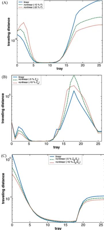
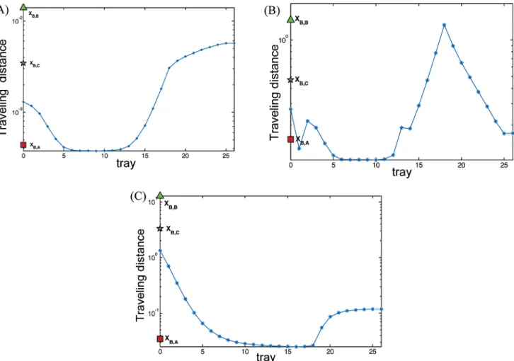
(8)

Figure 11. Traveling distance from linear analysis and nonlinear

(8)

where xj,iis the molar fraction of the component i of the

jth tray, Tjis the temperature of the jth tray, Gj,iis the

process transfer function of the component i of the jth tray, GTj is the process transfer function of the jth

temperature-control tray, GLj,i is the load transfer function of the component i of the jth tray, GLTjis the

load transfer function of the jth temperature-control tray, u is the manipulated variable, and d is the load variable.

Under the assumption of perfect temperature control,

we can get the value of the manipulated variable under closed-loop control.

This leads to

Then,

We define the absolute traveling distance as

The normalized traveling distance is

Figure 11A shows a plot of the traveling distance for a change in F. The solid line is computed from the linear analysis (eq 15), the dashed line is obtained from the nonlinear column simulation for a -10% F change, and the dotted line is also the result of the nonlinear simulation with a -20% feed flow change. Qualitatively similar shapes can be seen in Figure 11A where T1 control gives a large traveling distance as compared to

T5and T10control. Note that here we intend to control bottoms composition with vapor boilup as the manipu-lated variable, so the trays of interest should lie below the feed tray (T1-T18). Figure 11B shows the traveling distance for a ZA change, and Figure 11C shows the traveling distance for a ZB/ZCchange. The time-domain behavior in Figure 10 can be explained by the quantita-tive measure, and the results indicate that, the smaller the traveling distance, the better it is for stabilizing the composition profile in the column. Compared to single-temperature control, the dual-end control provides a much more critical test for the appropriateness of the temperature-control trays, and this is understandable because two temperatures are restricted on the iso-therms (e.g., Figure 14).

2.5. Dual-End Control. If we now consider dual-end control, where we use two column temperatures to control distillate and bottoms purities, we can look at how we select the two temperatures. Using the non-square relative gain (NRG),4 _{we would choose the top} temperature-control tray on theoretical stage 19. We will use two choices for the bottoms temperature-control trays on stage 1 or 9. The NRG is used for the measurement selection.

Here, ΛN _{stands for the NRG, X denotes} element-by-element multiplication, the superscripts T and + cor-respond to transpose and pseudo-inverse, respectively. Figure 12 shows the row sum of the NRG for the dual-end temperature-control problem. The analysis shows that T9 and T19 are the recommended temperature-control trays. Again, the concept of traveling distance can be used to explore the potential problem in dual-temperature control.

The traveling distance for dual-end control can be derived from the open-loop transfer function. Consider the following process transfer function matrices.

|∆x|2 |d|2 /NT

|

[(GL1,1 / )2+ (GL1,2 / )2]1/2 l [(GLNT,1 / )2+ (GLNT,2 / )2]1/2

|

2 /NT (15) ΛN) K X (K+)T (16)

[

x1,1 l xNT,1 x_1,2 l xNT,2 T₁ l T_NT

]

)

[

G_1,1(1) l GNT,1 (1) G1,2 (1) l GNT,2 (1) G_T 1 (1) l G_TNT(1) G_1,1(2) l GNT,1 (2) G1,2 (2) l GNT,2 (2) G_T 1 (2) l G_TNT(2)

]

)

]

[d] )

[

GL1,1 / l G_LNT,1/ GL1,2 / l GLNT,2 /

]

[d] (13) ∆xj) (

∑

i)1 NC-1 x_j,i2)1/2) (x_j,12+ x_j,22)1/2 (14)

(9)

where xj,iis the molar fraction of the component i of the

jth tray, Tjis the temperature of the jth tray, Gj,i(k)is

the process transfer function of the component i of the

jth tray under the kth manipulated variables, G_T

j

(k) _is the process transfer function of the jth temperature-control tray under the kth manipulated variable, GLj,i is the load transfer function of the component i of the

jth tray, and GLTj is the load transfer function of the

jth temperature-control tray.

If Tland Tmare under perfect control,

we can get

Substituting u₁CLand u₂CL into eq 18 and rearranging, we have

The traveling distance for dual-end control becomes

Figure 13 shows the traveling distance for dual-end control for F, ZA, and ZB/ZC changes. Here, we limit ourselves to the pairing of the lower part of the tem-peratures (below feed tray) with vapor boilup and the Figure 12. Row sum of NRG for dual-end temperature control

using reflux flow and vapor boilup as manipulated variables.

T_l) G_T l (1) u₁+ G_T l (2) u₂+ G_LT ld ) 0 T_m) G_T m (1) u₁+ G_T m (2) u₂+ G_LT md ) 0 (18) u₁CL) (-G_T m (2) G_LT l+ GLTmGTl,2) (GT_l (1) GT_m (2) _{- G} T_l (2) GT_m (1) ) d u2 CL₎(-GTl (1) GLT_m+ GLl,1GT_m (1) ) (GT_l (1) GT_m (2) _{- G} T_l (2) GT_m (1) ) d (19)

[

x1,1 l x_NT,1 x_1,2 l xNT,2

]

)

[

GL1,1 / l G_LNT,1/ G_L1,2/ l G_LNT,2/

]

[d]

Figure 13. Traveling distance for dual-end control with: (A) F,

(B) ZA, and (C) ZB/ZCchanges. |∆x|2 |d|2 /NT )

|

[(G_L1,1/ )2+ (G_L1,2/ )2]1/2 l [(G_LNT,1/ )2+ (G_LNT,2/ )2]1/2

|

2 /NT (20)

(10)

upper part of the temperatures (above feed tray) with reflux flow rate. The quantitative measure clearly shows that, indeed, T9and T19are better choices as compared to, for example, T1and T19. Rigorous nonlinear simula-tion indicates that dual-end control by keeping T9and

T19constant gives good composition dynamics, as shown in Figure 14, where the profile of component B reaches steady-state in 10 min for a 10% increase in ZB/ZC. On the other hand, the T1and T19dual-end control fails to stabilize the column for the same disturbance, as can be seen in Figure 15. The reason is that the increase in the intermediate boiler (component B) shifts the profile upward in the composition space (e.g., Figure 14A). It is not possible to hold tray 1 temperature at setpoint (not letting excess B out of the system) while maintain-ing tray 19 temperature at setpoint. If these two tem-peratures (T1and T19) are used, one way to avoid

insta-bility is to use proportional-only temperature control or to change the value of the controller setpoint.

2.6. Interaction between “Process” and “Con-trol” Direction. Why does T1control (single- or dual-end) result in a large traveling distance and, conse-quently, sluggish response? For temperature control, the “control direction” is fixed to the temperature isotherm, as shown in Figure 10. Regardless of the types of disturbances, that implies the composition on tray 1 has to lie on that isotherm. The process, on the other hand, generally moves along the tangent of the composition profile (distillation line), the “process” direction. Let us take the -20% feed flow change in Figure 10 as an example. The disturbance pushes the tray 1 composition further down toward the C corner along the B-C edge (the process direction). The T1 control, however, tries to move the tray 1 composition away from the B-C edge Figure 14. Reshaping composition profile with T9- T19control for +10% ZB/ZCchange for: (A) initial & final composition profiles with

traveling distance (shown by arrow) and (B) snapshots of composition profile of B as time approaches 0, 10, 30, and∞.

Figure 15. Internally unstable closed-loop responses with T1- T19control for +10% ZB/ZCchange.

(11)

along the T1 isotherm (the control direction), but not by much (because little A remains in the lower part of the column). Because a smaller amount of heavies than necessary is allowed to leave the column base, we have a build-up of B and C in the column that has to per-colate through to the composition redistribution, as can be seen in Figure 10. Certainly, the feed flow is altered, so we need to change the process direction. Relatively speaking, the conflict between the process and control directions is less severe for T10 control because of better maneuverability for tray 10 composi-tion. The interaction between the process and control directions is not limited to temperature control only; it can become even more severe for direct composition control.

3. Extension to Composition Control

3.1. Control Direction for Composition Con-trol. Composition control in multicomponent sys-tems differs from the binary system, since we have the freedom to select the controlled variable (e.g., purity, impurity, ratio of key components, etc.). This affects the control direction, as shown in Figure 16. When composi-tion A is under control (xjA ) constant), the control

direction is parallel to the B-C edge. Similarly, we can move the control direction perpendicular to the B-C edge by controlling xjBor we can make it parallel to the

A-B edge by keeping xjCconstant.

3.2. Single-End Control. Similar to the case of temperature control, the traveling distance for single-end composition control can be derived analy-tically, provided we have the steady-state gain matrices.

Assume xj,iis under perfect composition control,

We can get

When we substitute uCL_{into eq 22 and rearrange, we} have

The traveling distance is

Let us use the bottoms composition control to il-lustrate the effect of the control direction (by choosing different components to control) on the closed-loop performance. First, the traveling distance for control-ling xB,A, xB,B, and xB,Care computed according to eq 26. Figure 17 reveals that, as expected, xB,Acontrol gives the smallest traveling distance for all three distur-bance, because the control direction coincides with the process direction. Also xB,Bcontrol will give the worst performance because of its large traveling distance, where xB,C control lies somewhere between the two. The traveling distances for composition control are put in the same graph with that of temperature con-trol. Rigorous nonlinear simulations show that the conflict between the process and control directions using

xB,B and xB,C gives more sluggish responses. This can be seen in the snapshots of the xj,Bcontrol

composi-tion profiles in Figure 18. Much larger traveling dis-tances are observed for xB,B and xB,C control. On the other hand, xB,A control leads to faster composition dynamics as a result of a much smaller traveling distance.

3.3. Dual-Composition Control. The traveling dis-tance for dual-end composition control can be derived from the open-loop transfer function in a similar way as above.

Figure 16. Control directions with xj,A, xj,B, and xj,Ccontrol in

the composition space.

|∆x|2 |d|2 /NT )

|

{(GL1,1 / )2+ (GL1,2 / )2}1/2 l {(GLNT,1 / )2+ (GLNT,2 / )2}1/2

|

2 /NT (25)

[

x_1,1 l xNT,1 x_1,2 l x_NT,2

]

)

[

G1,1 (1) G1,1 (2) l l GNT,1 (1) GNT,1 (2) G1,2 (1) G1,2 (2) l l G_NT,2(1) G_NT,2(2)

]

)

]

[d] )

[

G_L1,1/ l G_LNT,1/ G_L1,2/ l G_LNT,2/

]

[d] (24)

(12)

Under perfect composition control by keeping the pth component of the lth tray and the qth component of the

mth tray constant, we have

Then

Substitute into

The traveling distance is

If xB,Acontrol resolves the conflict between the process and control directions at the bottom, we should expect control of composition C, xD,Cat the column top, to have similar behavior, which can be seen in Figure 16 where the control direction moves along the A-B edge as the upper section of the composition profile does. However, unlike dual-end temperature control, dual-composition control is able to reestablish the composition profile if one of the controlled compositions is correctly selected. This is because the component material balance con-straint has to be met. For example, if xB,Acontrol is used for the bottoms loop, the traveling distance is of the same order of magnitude regardless of which composi-tion is selected to control on the top loop (xD,A, xD,B, or

xD,C), as shown in Figure 19 for all three disturbances. The initial and final composition profiles for xB,A- xD,C control and xB,A- xD,Bcontrol in Figure 20 confirm that the traveling distances are almost the same for both cases. However, the snapshots of the profiles of B in the second row of Figure 20 indicate that xB,A- xD,Bcontrol goes through a much larger deviation as compared to the intuitively correct xB,A- xD,Ccontrol. Actually, the initial and final composition profiles almost coincide with each other for these two cases.

The time domain simulations for (20% feed flow rate changes in Figure 21 clearly indicate drastically differ-Figure 17. Traveling distance for different composition control (xB,A, xB,B, and xB,C) as compared to temperature control for: (A) F, (B) ZA, and (C) ZB/ZCdisturbances. x_l,p) G_l,p(1)u₁+ G_l,p(2)u₂+ G_Ll,pd ) 0 xm,q) Gm,q (1) u1+ Gm,q (2) u2+ GLm,qd ) 0 (27) u1 CL₎(-Gm,q (2) G_Ll,p+ G_Lm,qG_l,p(2)) (Gl,p (1) Gl,p (2)_{- G} m,q (1) Gm,q (2) ) d; u2 CL₎(-Gl,p (1) GLm,q+ GLl,pGm,q (1) ) (G_l,p(1)G_l,p(2)- G_m,q(1)G_m,q(2)) d (28)

[

x1,1 l x_NT,1 x1,2 l x_NT,2

]

)

[

G_L1,1/ l G_LNT,1/ G_L1,2/ l GLNT,2 /

]

[d] (29) |∆x|2 |d|2 /NT )

|

[(G_L1,1/ )2+ (G_L1,2/ )2]1/2 l [(GLNT,1 / )2+ (GLNT,2 / )2]1/2

|

2 /NT (30)

(13)

ent speeds of response for these two control structures, despite having almost the same final steady-state. The dual-composition control example points out the possible

limitation of the traveling distance analysis. Because the measure is computed from steady-state gain matri-ces, it only serves as a sufficient condition for control Figure 18. Reshaping composition profile for -10% ZB/ZCchange with (A) xB,Acontrol, (B) xB,Bcontrol, and (C) xB,Ccontrol: (top) initial

and final composition profiles with traveling distance (shown by arrow) and (bottom) snapshots of composition profile of B as time approaches 0, 10, 30, and∞.

Figure 19. Traveling distance under dual-composition control with different composition combinations for: (A) F, (B) ZA, and (C) ZB/ZC

(14)

performance evaluation. That is, we should eliminate the control (temperature or composition) with a large

traveling distance, but there is no guarantee that a small traveling distance leads to tight composition Figure 21. Closed-loop responses for (20% F changes with (A) xB,A- xD,Cand (B) xB,A- xD,Bcontrol.

Figure 20. Reshaping composition profile for -20% F change with (A) xB,A- xD,Ccontrol and (B) xB,A- xD,Bcontrol: (top) initial and

final composition profiles with traveling distance (shown by arrow) and (bottom) snapshots of composition profile of B as time approaches 0, 10, 30, and∞.

(15)

responses. However, this example clearly illustrates that consistent process and control directions do help to improve composition control.

4. Conclusions

For ternary distillation columns, if the maximum in the intermediate boiler composition profile lies below the feed, then we want to select a temperature-control location on the “upstream” side of the peak (i.e., between the feed point and the maximum). By doing this, we stabilize the temperature and composition profiles. If we select a temperature-control point on the other side of the peak, then changes in the column feed composi-tion will cause the intermediate boiler composicomposi-tion profile to wander away from its normal look in the region between the feed point and the maximum. As the intermediate component accumulates or is depleted on these trays, control of the column product composition will be poorer than when the profile is stabilized.

This phenomenon is quantified using the traveling distance that can be derived from steady-state gain matrices. It can be further explained by understanding the potential conflict between the process and control directions that govern the physical behavior in a mul-ticomponent distillation column. Unlike the uniform control direction determined by the temperature iso-therm (Figure 9), in multicomponent distillation, direct composition control allows us to choose the control direction in the top and bottom of the column (Figure 16). The quantitative measure, the traveling distance, is extended to single-end and dual-composition control to eliminate inappropriate components for control pur-poses. This affects the potential requirements for and benefits of an on-line composition analyzer. Then, preference is given to the control structure with con-sistent process and control directions. This two-step procedure is validated for single-end and dual-composi-tion control using rigorous nonlinear simuladual-composi-tions. Acknowledgment

We thank J. K. Chen and X. G. Shen for preparing some of the figures.

Nomenclature

Ai) Antoine coefficient for component i

B ) Antoine coefficient (same for all components) d ) load variable representing F, ZA, or ZB/ZCchanges F ) feed flow rate

G_j,i(k)) process transfer function of component i of the jth

tray (xj,i) under kth manipulated variable (uk)

GLj,i) load transfer function of component i of the jth tray (xj,i) under load variable d

G_T j

(k)_{) process transfer function of the temperature of the} jth tray (Tj) under kth manipulated variable (uk)

GLTj) load transfer function of the temperature of the jth

tray (Tj) under load variable d

Ki) equilibrium constant (K-value) for the ith component

NC ) number of component NRG ) nonsquare relative gain NT ) total number of trays

P ) pressure

Pi0) reference vapor pressure

Pi

sat_{) vapor pressure of component i} T ) temperature

Tj) jth tray temperature

T0) reference temperature

T_Csat ) boiling point temperature of component C at a

given pressure

uj) jth manipulated variable

uCL _{) steady-state value of manipulated variable under}

perfect control

xi) liquid-phase composition of ith component

xj,i) ith component liquid-phase composition on jth tray

yi) vapor phase composition of ith component

Zi) feed composition of ith component

Greek Symbols

R_i_{) relative volatility of component i} ∆H ) heat of vaporization

∆xj) traveling distance of tray j composition

Literature Cited

(1) Rademaker, O.; Rijnsdorp, J. E.; Maarleveld, A. Dynamics

and Control of Continuous Distillation Units; Elsevier: New York,

1975.

(2) Buckley, P. S.; Luyben, W. L.; Shunta, J. P. Design of

Distillation Column Control Systems; Instrument Society of

America: Research Triangle Park, NC, 1985.

(3) Downs, J. J.; Moore, C. F. Steady-State Gain Analysis for

Azeotropic Distillation. Proceedings JACC, Charlottesville, VA,

1981; Paper WP-7C.

(4) Chang, J. W.; Yu, C. C. The Relative Gain for Nonsquare Multivariable Systems. Chem. Eng. Sci. 1990, 45, 1309.

(5) Cao, Y.; Rossiter, D. An input pre-screening technique for control structure selection. Comput. Chem. Eng. 1997, 21, 563-569.

(6) Yu, C. C.; Luyben, W. L. Use of Multiple Temperatures for the Control of Multicomponent Distillation Columns. Ind. Eng.

Chem. Process Des. Dev. 1984, 23, 590-597.

(7) Joseph, B.; Brosilow, C. B. Inferential Control Of Process EM DASH 1. Steady-State Analysis and Design. AIChE J. 1978,

24, 485-492.

(8) Skogestad, S.; Mejedll, T. Estimation of distillation composi-tion from multiple temperature measurements using PLS regres-sion. Ind. Eng. Chem. Res. 1991, 30, 2543-2555.

(9) Kano, M.; Miyazaki, K.; Hasebe, S.; Hashimoto, I. Inferen-tial control system of distillation compositions using dynamic partial least squares regression. J. Process Control 2000, 10, 157-166.

(10) Kano, M.; Showchaiya, N.; Hasebe, S.; Hashimoto, I. .Inferential control of distillation compositions: Selection of model and control configuration. Control Eng. Pract. 2003, 11, 927-933. (11) Pannocchia, G.; Brambilla, A. Consistency of Property Estimators in Multicomponent Distillation Control. Ind. Eng.

Chem. Res. 2003, 42, 4452-4460.

(12) Luyben, M. L. Impact of Plantwide Design on Control of an Industrial Distillation Column. Presented at National Taiwan University, Taipei, Taiwan, 2002.

(13) Luyben, W. L. Process Modeling, Simulation and Control

for Chemical Engineers, 2nd ed.; McGraw-Hill: New York, 1990.

(14) Shen, S. H.; Yu, C. C. Use of Relay-Feedback Test for Automatic Tuning of Multivariable Systems. AIChE J. 1994, 40, 627-645.

(15) Luyben, W. L. Tuning Proportional-Integral-Derivative Controllers for Integrator/Deadtime Processes. Ind. Eng. Chem.

Res. 1996, 35 (10), 3480-3483.

(16) Hwang, Y. L. Nonlinear Wave Theory for Dynamics of Binary Distillation Columns. AIChE J. 1991, 37, 705-723.

(17) Kienle, A. Low-order dynamic models for ideal multicom-ponent distillation processes using nonlinear wave propagation theory. Chem. Eng. Sci. 2000, 55, 1817-1828.

Received for review February 3, 2005 Revised manuscript received August 10, 2005 Accepted August 19, 2005 IE050130M

Interpretation of Temperature Control for Ternary Distillation

Article

Interpretation of Temperature Control for Ternary Distillation

Min-Te Lin, Cheng-Ching Yu, and Michael L. Luyben

More About This Article

Interpretation of Temperature Control for Ternary Distillation

(

)

(

)

(

)

∑

[

(

)

]

∑

∑

∑

∑

∑

[

(

)

]

{

[

(

)

]

}

|

|

[

]

[

]

[

]

[

]

[

]

[

]

[

]

(

)

(

)

[

]

[

(

)

(

)

(

)

(

)

]

[

]

∑

[

]

[

]

|

|

|

|

[

]

[

]

[