IEEE SIGNAL PROCESSING LETTERS, VOL. 12, NO. 2, FEBRUARY 2005 89
Direct N-Point DCT Computation From Three
Adjacent N/3-Point DCT Coefficients
Soo-Chang Pei, Fellow, IEEE, and Meng-Ping Kao
Abstract—An efficient method for computing a length- Dis-crete Cosine Transform (DCT) from three consecutive length- 3 DCTs is proposed. This method differs from previous ones in that it reduces considerable 31–38% arithmetic operations and uses only length- 3 DCTs instead of length- DCTs. We also find its great applications in fractional scaling of a block DCT-based image by the factor of1 2 3 . This would be very useful in high-definition television (HDTV) standard, whose display size is usually 16:9. The comparison with conventional methods is provided in this paper.
Index Terms—Direct DCT domain computation, fast DCT, radix-3 DCT.
I. INTRODUCTION
S
INCE the Discrete Cosine Transform (DCT) was first in-troduced in 1974, it has been widely used in various fields among digital signal processing (DSP). For example, it is the foundation of many prevailing image and video compression techniques, such as JPEGs, MPEGs, and H.26x. Moreover, most of the images and videos nowadays are stored in the DCT do-main through the above techniques. The following question, however, arises: How can we directly manipulate or process such a compressed media stored in the DCT domain?To avoid unnecessary computations in decompression and re-compression, a number of algorithms have been proposed to complete the operations directly in the DCT domain. Among the various operations, scaling of an image, i.e., interpolation or decimation, is probably the most common one we might en-counter in relevant applications. For example, Park [4] has pro-posed an algorithm using the symmetric convolution property of DCT. Zhao [5] utilizes the relationship between linear trans-forms in spatial domain and those in DCT domain to develop an alternative approach.
However, as long as an ideal scaling operation is concerned, it is necessary to construct a long DCT sequence from several short DCT sequences or to decompose a long DCT sequence into several short DCT sequences in the compressed domain. For example, when the decimation operation is concerned, it is
Manuscript received March 24, 2004; revised June 14, 2004. This work was supported by the National Science Council, R.O.C., under Contracts NSC93-2219-E-002-004 and NSC93-2752-E-002-006-PAE. The associate editor coor-dinating the review of this manuscript and approving it for publication was Dr. Markus Pueschel.
The authors are with the Department of Electrical Engineering, National Taiwan University, Taipei, Taiwan 10617 R.O.C. (e-mail: [email protected]; [email protected]).
Digital Object Identifier 10.1109/LSP.2004.840868
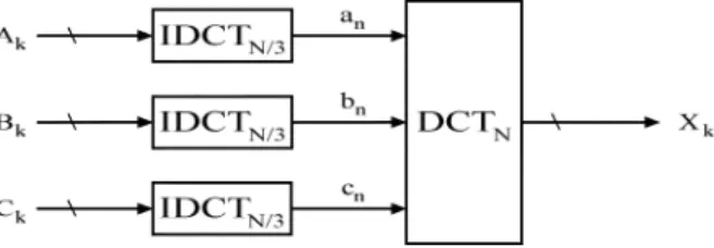
Fig. 1. Schematic representation of the traditional approach.
straightforward to reserve the low-frequency components and discard the high-frequency ones from the long DCT sequence, which is comprised by several short, original DCTs. On the other hand, when the interpolation operation is concerned, we should first zero-pad a short DCT to its high-frequency band and then split the resulting long DCT to several short DCTs to complete the interpolation. Readers could refer to [4] for more details.
Since Skodras [1] has proposed a corresponding method for the case of two sequences, we now focus on the case of three consecutive sequences in this paper. Combining with Skodras’s method, many DCT domain operations, such as fractional scaling by the factor of , are now realizable in a simple and efficient way.
II. CONVENTIONALAPPROACH
Let us readdress the problem as follows. Assume a length sequence is composed of three consecutive sequences with
length , i.e., , , and
for , and , , and are their length
DCT coefficients, respectively. Given , , and , how can we find an efficient way to compute the length DCT co-efficients ?
The conventional way to solve this problem is depicted in Fig. 1. According to this scheme, three -point IDCTs are required, followed by a -point DCT. Even if the fast -point DCT structure using three -point DCTs [2] is applied to simplify the -point DCT, however, the total computational complexity in Fig. 1 is still limited by at least six -point DCTs.
In order to modify the conventional approach, we propose a new structure based on DCT decomposition to avoid the -point DCT computation. In this way, we use only four -point DCTs to find , which is much more efficient than before.
1070-9908/$20.00 © 2005 IEEE
90 IEEE SIGNAL PROCESSING LETTERS, VOL. 12, NO. 2, FEBRUARY 2005
Now, we go straight to investigating the key concept of this new structure. First of all, the normalized forward DCT-II of length- sequence is given as follows:
(1) and the corresponding inverse DCT is
(2) where
for
for (3)
Note that and . We now
decom-pose into three equal-length parts , , and , respectively, according to [2]. That is
(4)
(5)
(6) where
(7) Note that in (5) and (6), when , and are defined in the same manner as that in (1). Moreover,
for ,
and . As a consequence
DCT DCT
for (8)
The decomposition method addressed above is categorized as “decimation in frequency.” Its computational complexity is given by the following equations in both recursive and nonre-cursive forms:
(9)
(10) There are, of course, other methods of decomposition, such as “decimation in time” or “mix decimation.” For example, Bi [6] has proposed an algorithm using the mix decimation method in which it has a minimum nine-point DCT complexity with and , where some operations on trivial factors are precluded. For details, please refer to [6]. In general, Bi’s method has the computational complexities as follows:
(11)
(12) We see from (9) and (11) that Chan’s method is more superior to Bi’s in that its multiplications are about less when the same nine-point DCT module are utilized for
. As a consequence, for practical implementation, we could combine Bi’s optimized nine-point DCT module [6] together with Chan’s N-point DCT decomposition for .
III. PROPOSEDAPPROACH
Since the DCT coefficients , , and are precomputed and saved in the compressed domain, the main difference be-tween the proposed method and the radix-3 DCT algorithm [2] is to merge three length DCT coefficients , , and into a length DCT very efficiently.
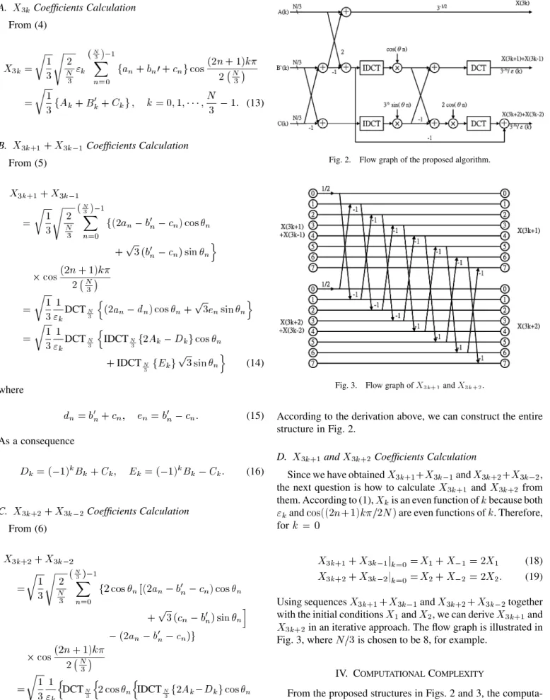
PEI AND KAO: DIRECT N-POINT DCT COMPUTATION FROM THREE ADJACENT N/3-POINT DCT COEFFICIENTS 91 A. Coefficients Calculation From (4) (13) B. Coefficients Calculation From (5) DCT DCT IDCT IDCT (14) where (15) As a consequence (16) C. Coefficients Calculation From (6) DCT IDCT IDCT (17)
Fig. 2. Flow graph of the proposed algorithm.
Fig. 3. Flow graph ofX andX .
According to the derivation above, we can construct the entire structure in Fig. 2.
D. and Coefficients Calculation
Since we have obtained and ,
the next question is how to calculate and from them. According to (1), is an even function of because both and are even functions of . Therefore, for
(18) (19)
Using sequences and together
with the initial conditions and , we can derive and in an iterative approach. The flow graph is illustrated in Fig. 3, where is chosen to be 8, for example.
IV. COMPUTATIONALCOMPLEXITY
From the proposed structures in Figs. 2 and 3, the
computa-tion of , , and requires
seven length- vector additions, three length- vector multiplications, and 4 length- DCTs, assuming that the
92 IEEE SIGNAL PROCESSING LETTERS, VOL. 12, NO. 2, FEBRUARY 2005
DCT and the indiscrete DCT (IDCT) are of the same
com-plexity. Furthermore, when , ,
, , and (14) and (17) become
DCT IDCT
IDCT
DCT IDCT
IDCT
Therefore, we can save two more multiplications. On the other hand, the computation of and in Fig. 3 requires 2 length- vector additions since multiplication by 1/2 can be implemented using a bit-wise shift operator.
For the purpose of simplicity, we choose in the following comparisons such that the fast DCT could be used to implement length- DCTs, where is a positive integer. According to [3], the arithmetic complexity of a
length-fast DCT is
(20) (21) The total numbers of multiplications and additions of the proposed structure in Fig. 2, then, become
(22)
(23) As for the conventional approach in Fig. 1, the complexity is equal to three length- DCTs and one length- DCT. The total numbers of multiplications and additions of the conventional structure, then, become [2]
(24)
(25) We summarize the computational complexity of these two ap-proaches in Table I. Note that the computational saving per-centage increases with . Specifically, when , the asymptotic saving percentages approach 50% for both multipli-cations and additions. Moreover, for , which is the standard block dimension for image and video coding, about 31–38% operations can be saved.
TABLE I
COMPUTATIONALCOMPLEXITIES OFCONVENTIONAL ANDPROPOSEDMETHODS
DESCRIBED IN(22)TO(25)
For the application of block-DCT-based image down-sam-pling, since the higher frequency DCT coefficients will virtually be discarded, there is no need to compute them in Figs. 2 and 3. Let us take the case of down-sampling by 3, for example. We need only to compute the first 1/3 terms. Therefore, two vector additions, i.e., the left-top and right-bottom additions in Fig. 2, can be replaced by length- vector additions. The two length- forward DCTs could be replaced by length-pruned DCTs (PDCT) of first terms. Moreover, the additions in Fig. 3 are also reduced to two
length-vector additions. The complexity of PDCT can be computed according to [8]. In this way, a huge amount of computations could be saved.
V. CONCLUSION
We propose an efficient approach to compute a length-DCT given three consecutive length- DCTs. The oper-ations could be saved from 31% up to 38% when the block size is chosen from 8 to 32, and the larger the block size, the more operations we can save. Another advantage is that only length- DCTs and IDCTs are required, instead of length- DCTs. Combining with Skodras’s method, scaling a DCT-based image by the factor of is easily realizable by cascading for Skodras’s structures and for the authors’ structures. This provides more flexibility and efficiency in the application of fractional scaling, especially in the rising standard of HDTV, whose screen size is usually set to be 16:9.
REFERENCES
[1] A. N. Skodras, “Direct transform to transform computation,” IEEE
Signal Process. Lett., vol. 6, no. 8, pp. 202–204, Aug. 1999.
[2] Y.-H. Chan and W.-C. Siu, “Fast radix-3/6 algorithms for the realization of the discrete cosine transform,” in Proc. IEEE Int. Symp. Circuits Syst., vol. 1, May 3–6, 1992, pp. 153–156.
[3] C. W. Kok, “Fast algorithm for computing discrete cosine transform,”
IEEE Trans. Signal Process., vol. 45, no. 3, pp. 757–760, Mar. 1997.
[4] H. W. Park, Y. S. Park, and S.-K. Oh, “L/M-fold image resizing in block-DCT domain using symmetric convolution,” IEEE Trans. Image
Process., vol. 12, no. 9, pp. 1016–1034, Sep. 2003.
[5] Y. Zhao, M. S. Kankanhall, and T.-S. Chua, “Fractional scaling of image and video in DCT domain,” in Proc. IEEE Int. Conf. Image Process., vol. 1, Barcelona, Spain, Sep. 14–17, 2003, pp. 185–188.
[6] G. Bi and L. W. Yu, “DCT algorithms for composite sequence lengths,”
IEEE Trans. Signal Process., vol. 46, no. 3, pp. 554–562, Mar. 1998.
[7] Y.-H. Chan and W.-C. Siu, “Mixed-radix discrete cosine transform,”
IEEE Trans. Signal Process., vol. 41, no. 11, pp. 3157–3161, Nov. 1993.
[8] A. N. Skodras, “Fast discrete cosine transform pruning,” IEEE Trans.
Signal Process., vol. 42, no. 7, pp. 1833–1837, Jul. 1994.