自我類化訊流的合成及分散式辨識

國

立

交

通

大

學

電子工程學系 電子研究所

博 士 論 文

自我類化訊流的合成及分散式辨識

Synthesization and Decentralized Identification

of Self-Similar Processes

研 究 生：姚 建

指導教授：蔣 迪 豪 博 士

陳 伯 寧 博 士

自我類化訊流的合成及分散式辨識

Synthesization and Decentralized Identification

of Self-Similar Processes

研 究 生：姚 建 Student：Chien Yao

指導教授：蔣迪豪 Advisor：Tihao Chiang

陳伯寧 Po-Ning Chen

國 立 交 通 大 學

電子工程學系 電子研究所

博 士 論 文

Submitted to Department of Electronics Engineering and Institute of Electronics

College of Electrical and Computer Engineering National Chiao Tung University

in partial Fulfillment of the Requirements for the Degree of

Doctor of Philosophy in Electronics Engineering July 2007 Hsinchu, Taiwan

2008 年 7 月

自我類化訊流的合成及分散式辨識

學生：姚 建

指導教授

蔣迪豪

陳伯寧

國立交通大學電子工程學系

摘

要

在本論文的第一部分，我們提出了一個濾波器型式的自我類化訊流合成器。此合

成器能生成可調控變異性及相關性的長程相依訊流，同時也只需很少的輸入參

數。與既有的其它自我類化訊流合成器﹙如 RMD 方法和 Paxson 的 IFFT 方法﹚相

比，我們提出的濾波器型式的自我類化訊流合成器具有能即時生成訊流以及生成

之訊流恆不為負值之優點。我們接著研究了相關係數﹙只能反映線性的相依關係﹚

和交互訊息﹙能測量一般的相依關係﹚兩者之間的蘊含關係。本研究的結果建議，

對於弱相關的隨機變數，如一個自我類化過程中具有長的時間差的不同二個時刻

的值，相關係數的平方值的一半似可作為交互訊息的一個合理的近似。

基於長尾分佈和自我類化訊流之間的存在的基本關係，我們進而研究了此類訊流

的分散式辨識問題。我們發現若干有趣的結果。首先，我們確證了全同感測器系

統在指數分佈族的參數辨識問題上的最佳性。在此研究方向上的一個相關的結果

是，在指數分佈族辨識問題上，串接式兩感測器系統和平行式兩感測器系統具有

相同的最佳性能。這多少是令人感到意外的，因為一般認為串接式兩感測器系統

比平行式兩感測器系統有更好的性能。

其次，對於更一般類別分佈族的參數辨識問題，我們提出數個命題可用來檢證全

同感測器系統的最佳性。如採取直捷的手法來檢證全同感測器系統，通常將導致

在被一組非線性聯立方程所定義的解空間之中搜尋所有的局域最小值。然而這種

方法在一些情況下會是不可行的，而我們提出的命題可作為一個較佳的替代方

案。此外，我們的研究也可應用到其它的分散式檢測問題上，如在倖存分析及損

壞時間分析的壽命問題上，或是如在利用在地理上分散設備，對不同連結上的封

包到達時間間隔加以量測，來決定整個網路的自我類化參數的問題上。

最後，藉由對函數及方程式的數值計算結果，我們確認了，在加法性高斯雜訊下

二元信號的檢測問題上全同感測器系統的最佳性。

Synthesization and Decentralized Identification

of Self-Similar Processes

student：

Advisors：Dr. Tihao Chiang

Dr. Po-Ning Chen

Department of Electronics Engineering and Institute of Electronics

National Chiao Tung University

ABSTRACT

In the first part of this dissertation, we propose a filter-based generator for the

synthesization of self-similar traffics. It can produce long range dependent traffics

with adjustable levels of bustiness and correlation, and is parsimonious in the number

of model parameters. By comparing it with existing self-similar traffic synthesizers,

e.g., the RMD and the Paxson IFFT algorithms, the proposed filter-based synthesizer

has the advantages that the synthetic traffic can be generated on the fly, and always

produces non-negative-valued traffic. The implications between the correlation

coefficient (a quantity that only measures the linear dependence) and mutual

information (a quantity that can represent the general dependence) is subsequently

investigated. The obtained results suggest that for weakly correlated random variables

such as two instances of a self-similar process with a long time lag, half the square of

the correlation coefficients might be a reasonable approximation to the mutual

information.

Continuing from the synthesization of processes with heavy tails, we turn to

study the impact of such processes on decentralized detection. Several interesting

results are found. Firstly, the optimality of identical sensor system for the exponential

distribution family has been verified. A side result along this research line is that

the optimal performance of the serial two-sensor system is the same as that of the

parallel two-sensor system for exponential sources. This is somewhat surprising

because it is generally considered that the serial two-sensor system has better

performance than the parallel two-sensor system.

Secondly, for a more general class of distribution families, we propose several

propositions on the optimality of the identical system. A straightforward approach to

test the optimality of identical sensor system often results in searching all local

minimums in the solution space that is defined through a set of nonlinear equations.

However, this approach is not tractable in certain situations. Our propositions then

provide an alternative for optimality test of identical sensor system. Besides, they can

be applied to other decentralized detection problems like the detection of lifetime

encountered in survival analysis and failure time analysis or the determination of the

degree of self-similarity of the whole network system based on geographically

dispersed measurements of the packet inter-arrival times on different links.

Finally, with the help of numerical study on functions and equations, we

analytically confirm the optimality of identical sensor system over Gaussian sources.

誌

謝

Contents

Abstract i

Acknowledgements iii

List of Tables vii

List of Figures viii

1 Introduction 1

1.1 Definitions of Self-Similar Processes . . . 4

1.2 Properties of Self-Similar Processes . . . 5

1.2.1 Range of Dependence . . . 5

1.2.2 1/f -Noise . . . . 6

1.2.3 Slowly Decaying Variance of Self-Similar Processes . . . 7

1.2.4 Heavy-Tailed Distribution . . . 7

1.2.5 Hurst Effect . . . 8

1.3 Decentralized Detection . . . 9

2 A FILTER-BASED SELF-SIMILAR TRACE SYNTHESIZER 12

2.1 Filter-Based Asymptotic Self-Similar Traffic Synthesizer . . . 13

2.1.1 Transfer Function In Self-Similar Traffic Synthesizer . . . 13

2.1.2 Impact On Self-Similarity Due To Filter Truncation . . . 18

2.1.3 Impact On Self-Similarity Due To Output Rounding . . . 19

2.2 The Reverse Filter Versus The Forward Filter . . . 21

2.3 Concluding Remarks . . . 22

3 Correlation Approximation to the Mutual Information of Self-Similar Pro-cesses 24 3.1 Introduction . . . 24

3.2 Definitions and Notations . . . 25

3.3 Main Theorems . . . 27

3.4 Examples . . . 31

4 Bayesian Decentralized Detection for Exponential Distributions 34 4.1 Preliminaries . . . 35

4.2 System with one sensor . . . 39

4.3 Parallel Two-sensor System . . . 40

4.4 The Parallel Sensor System with an Additional Broadcast Sensor . . . 42

4.4.1 The Serial Two-sensor System . . . 44

4.5 The Ξn System . . . 47

4.7 The Parallel Three-sensor System . . . 56 4.8 Problems with Similar ROCs . . . 59 4.8.1 Decentralized Classification of Heavy-tailed Sources Problems . . . . 62 4.9 Gaussian Classification Problems . . . 63

5 Conclusions 65

5.1 Self-Similar Traffic Generators . . . 65 5.2 Correlation Approximation to the Mutual Information of Self-Similar Processes 66 5.3 Bayesian Decentralized Detection . . . 66

References 68

List of Tables

2.1 Comparison between the resultant Hurst parameters of the traces synthesized by the filter-based algorithm and the targeted ideal Hurst parameters. . . 21

List of Figures

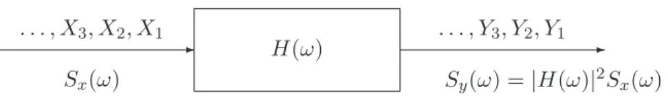
2.1 Relation between the power spectral densities of the filter input and filter

output random processes. . . 13

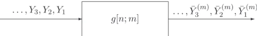
2.2 The variance-equivalent m-averaged process. . . . 15

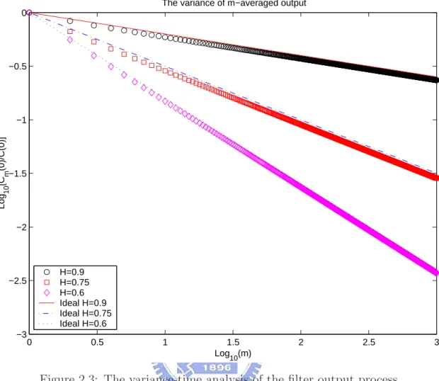
2.3 The variance-time analysis of the filter output process. . . 17

2.4 The lower and the upper bounds of log[Cm(0)/C1(0)]. . . 18

2.5 The variance-equivalent m-averaged process of the truncated filter output pro-cess. . . 19

2.6 Variance-time analysis (log₁₀ scale) for the truncated-filter output with trun-cation window W = 103_{. The slope of the solid line is equal to 2H − 2 for} m ≤ W , and −1 for m > W . . . . 20

2.7 The proposed asymptotic self-similar traffic synthesizer. H(w; W ) represents a truncated version of H(ω) with truncation window W . The quantity bYi+0.5c equals the closest integer to Yi. . . 21

2.8 Variance-time plots (log₁₀scale) for the two filter-based synthetic arrivals with truncation window 104 _{and mean rate 1. . . . 23}

3.1 The bounds and minimum mutual information for Gaussian distributed PX and PY. . . 33

Chapter 1

Introduction

Stationary random processes, according to their autocorrelation functions, can be classified as either short-range or long-range dependence. The former have summable autocorrelation functions, while the latter have non-summable autocorrelation functions. The simulations of the short-range dependent random processes have attracted attention for years, and have found many applications such as the traffic model of telecommunication systems [6]. How-ever, researchers had recently found that the traffic in many modern communications, such as the world wide web [4, 8, 14, 18, 20] and variable-bit-rate (VBR) video transmission [10], is significantly different from the conventional short-range dependent traffic models, and ex-hibit the renowned self-similar nature. This arouse the demand for the synthesization of processes with long-range dependence.

In literature, there have been several approaches proposed for the synthesization of long-range-dependent self-similar traffics. They include methods based on fractional Gaussian noise [14], M/G/∞ queue model [12], autoregressive processes [3], wavelet [2], . . ., etc. These synthesizers can be roughly divided into two categories: approaches derived from “time-domain” aspect and ones developed from “frequency-“time-domain” standpoint. An example for the former is the random-midpoint displacement (RMD) algorithm proposed by Lau et al. [13], while the spectrum fitting to the fractional Gaussian noise, as proposed by Paxson [19],

can be a typical synthesizer for the latter.

The procedures of the RMD algorithm is to recursively subdivide the present time in-tervals, and generate in each subdivision a new mid-point traffic data based on the end-point data obtained in the previous subdivision. This method can efficiently generate a well-approximated fractal Brownian motion (FBM) sequence. It however comes with the drawbacks that only the FBM traffics can be synthesized, and the desired amount of traffic has to be specified in advance.

Based on the power spectrum fitting to the fractional Gaussian noise (FGN), Paxson proposed a fast self-similar traffic generator using the inverse discrete-time Fourier transform (IDTFT), which is usually referred as the FFT method. By using an approximate form of the spectrum density of fractal Gaussian noises (FGN), a random sequence is formed in frequency domain. An inverse Fourier transformation (IFFT) is then performed to transform the sequence from the frequency domain to the time domain. The FFT algorithm improves the RMD algorithm in speed. In particular, the FFT algorithm only takes half time of the RMD algorithm for the same sequence length. Again, its drawback is that the traffic sequence cannot be generated on the fly. In addition, the simplified form of the FGN spectrum causes the resultant degree of self-similarity deviated from the target one.

In applying the aforementioned approaches to the generation of self-similar traces, several problems can be encountered. Firstly, the required length (i.e., amount) of traffic data must be priorly determined; hence, when a longer traffic sequence is required, one has to drop the existing data, and re-generate a completely new trace of the required length. Secondly, the required traffic data must be generated in an off-line fashion before they can be put to use. This somewhat restricts their usage in situation where on-the-fly traffic synthesizers are needed. Thirdly, these traffic generators may produce negative number, which is an undesired value for, say, packet-train arrivals. The direct elimination of these

negative-valued data however may make the degree of self-similarity of the generated trace deviating from the target one.

In this work, we propose a model that can produce long-range dependent sequences with adjustable levels of bustiness and correlation. When it is compared to the two known self-similar traffic generators—the RMD and the Paxson FFT, our model provides additional advantages that the synthetic traffic can be generated on the fly, and is always non-negative. Although the variance-time analysis shows that the filter length W limits the valid aggre-gation size of self-similarity, this phenomenon turns out to match the measured behavior of true network traffic, where the self-similar nature only lasts beyond a practically manageable range, but disappears as the considered aggregated window is much further extended, e.g., Beran et al. [4, Fig. 2].

The relationship between the second-order statistics (which are used in the measurement of the self-similarity in the network traffic) and the quantities in the information theory is also an interesting topic. Since one might expect that the self-similar traffic has some special characteristics that can be easily identified in the information processing of the measured data, we discuss the relationship between the correlation coefficients and mutual information in Chapter 3.

For the practical control of network traffic, one might need to test whether its self-similarity is weak or strong enough that the long-range dependence could or could not be ignored. To reduce the response time and to alleviate the load of network, a decentralized scheme for the detection of the self-similarity might be useful. In this work, we consider the decentralized detection, especially on the optimal design of the local decision rules and the fusion rule for the classification of exponential sources. It turns out that the optimal strategy is to use identical sensors and k-out-of-n fusion rule. We also show for such classification problem that the optimal performance of the serial two-sensor system is the same as the

optimal parallel two-sensor system. In addition, we address a set of propositions on the optimality of the identical sensor system, which can be verified without much difficulty. Some generalizations are further established and remarked for the decentralized detection of Gaussian sources, and for the determination of degree of self-similarity via the local measurements of packet inter-arrival durations.

1.1

Definitions of Self-Similar Processes

Self-similar processes were first introduced by Mandelbrot and his co-workers in 1968 [15, 16, 17]. These processes were thereafter found applications to many fields such as astronomy, chemistry, economics, engineering, mathematics, physics, statistics, etc. Recently, mea-surement studies have shown that the actual traffic from computer networks is long-range dependent [14, 18, 8, 4, 20], and thus another new application of self-similar processes was initiated.

Assume a second-order stationary real-valued stochastic process Y , {Yi}i∈I1 with finite

marginal mean µ and marginal variance σ2_{, where I}

j , {j, j + 1, j + 2, . . .}. Denote by

Y(m) _{, {Y}(m)

i }i∈I1 the m-averaged process of Y , where for m, i ∈ I1,

Y_i(m), 1 m m X j=1 Ym(i−1)+j.

Let the autocovariance and autocorrelation coefficient function of the m-averaged process

Y(m) _{be denoted by C}

m(k) , Cov{Yi(m), Y

(m)

i+k} and ρm(k) , Cm(k)/Cm(0), respectively. For notational convenience, the subscript of ρm(·) will be dropped when m = 1. Then, several variants of self-similarities can be defined as follows.

Definition 1.1. [24] A strictly stationary process Y is called strictly self-similar with pa-rameter H = 1 − (β/2), where 0 < β < 1, if

where “=” means that the equality is taken in the sense of finite-dimensional distributions.d Definition 1.2. [24] A second-order stationary process Y is called exactly second-order

self-similar with parameter H = 1 − (β/2), where 0 < β < 1, if either of the following conditions

holds: ρ(k) = 1 2[|k + 1| 2H_{− 2|k|}2H _{+ |k − 1|}2H_{], k ∈ I} 1 (1.2) Cm(k) = C1(k)m−β, k ∈ I0, m ∈ I1 (1.3)

Notably, (1.2) and (1.3) are indeed equivalent. Also note that (1.2) implies that ρm(k) =

ρ1(k) for m ∈ I1.

Definition 1.3. [24] A order stationary process Y is called asymptotically

second-order self-similar with parameter H = 1 − (β/2), where 0 < β < 1, if

lim k→∞ρm(k) = 1 2[|k + 1| 2H _{− 2|k|}2H_{+ |k − 1|}2H_{], m ∈ I} 1. (1.4)

The parameter H in the above definitions is usually referred to as the Hurst parameter. For other variant definitions of self-similar processes, see [24] and [25].

1.2

Properties of Self-Similar Processes

In this section, we summarize the statistical properties of self-similar processes that are of use in this work.

1.2.1

Range of Dependence

Random processes can be classified into two groups: short-range dependence (SRD) and

long-range dependence (LRD). Their formal definitions that have been appeared in the literature

Definition 1.4. [24] [7] A process Y is said to be short-range dependent, if ∞

X k=−∞

|ρ(k)| < ∞ (1.5)

Definition 1.5. [24] [7] A process Y is said to be long-range dependent, if ∞

X k=−∞

|ρ(k)| = ∞ (1.6)

A variant definition of long-range dependence is defined as follows. Definition 1.6. [22] A process Y is said to be long-range dependent, if

lim k→∞

ρ(k)

L(k)k2H−2 = 1, (1.7)

where L(k) is a slowly varying function at infinity, defined by lim

k→∞

L(kx)

L(k) = 1 for all x > 0. (1.8)

For an exact second-order self-similar process Y, its autocorrelation coefficient function is given by equation (1.2), i.e.,

ρ(k) = 1

2[|k + 1|

2H _{− 2|k|}2H _{+ |k − 1|}2H_{], k ∈ I} 1.

Using Taylor expansion, we obtain

ρ(k) = H(2H − 1)k2H−2_{+ o(k}2H−2_{), k ∈ I}

1, 0.5 < H < 1.

Therefore, an exact second-order self-similar process is indeed long-range dependent in the sense of Definition 1.6.

1.2.2

1/f -Noise

1/f -noise is the term used to present a sharp divergence in the power spectral density around the origin. The exact definition of 1/f -noise is in the following.

Definition 1.7. [22] A stationary process Y is said to present 1/f -noise, if its power spectral density S(ω) satisfies: lim ω→0 S(ω) L(1/ω)ω1−2H = 0, (1.9)

where L(k) is a slowly varying function at infinity (cf. (1.8)), and Hurst parameter H is in the range of (0.5, 1).

It has been proven that the long-range dependence in the sense of Definition 1.6 is equivalent to 1/f -noise [3, pp. 53].

1.2.3

Slowly Decaying Variance of Self-Similar Processes

In the case of short-range dependence or independence, the variance of m-averaged process decreases as the reciprocal of the average size, m. However, by equation (1.3),

Var{X(m)_{} = C}

m(0) = C1(0)m−β = Var{X}/m2−2H, (1.10)

and the variance of m-averaged processes decreases more slowly than the reciprocal of the average size, m, for long-range dependent processes. In fact, (1.10) indicates that Var{X(m)_} decreases as a slop of (2H − 2) in log-log plot against m.

1.2.4

Heavy-Tailed Distribution

Definition 1.8. A random variable Y is said to be heavy-tailed with parameter α ≥ 0, if

lim y→∞

Pr{Y > y}

L(y)y−α = 1, (1.11)

where L(x) is a slowly varying function at infinity (cf. (1.8)).

Here, we only concern the cases of 1 < α < 2, i.e., the mean of random variable Y is finite, and its variance is infinite. The infinite variance can be regarded as an extremely

variable phenomenon. This kind of heavy-tailed random variable has been used to model the arrival time of network packets. It has been shown [11] that if the packet inter-arrival process is modelled as i.i.d. Pareto random variables,1 _{the packet counting process is} asymptotically second-order self-similar process with H = (3 − α)/2, where parameter α is in the range of (0, 1) and (1, 2).

1.2.5

Hurst Effect

Historically, self-similar processes are marked because these processes provide an elegant interpretation of the empirical phenomenon, usually referred to as the Hurst Effect.

Given a series of observations Y1, Y2, Y3, · · · with sample mean µ(n) = (1/n) P_n j=1Yj and sample variance S(n) = 1 n n X j=1 [Yj − µ(n)]2,

the re-scaled adjusted range (or conventionally, the R/S statistics) is defined as

R(n) S(n) = max1≤k≤n hP_k j=1Yj − kµ(n) i − min1≤k≤n hP_k j=1Yj− kµ(n) i S(n) . (1.12)

Hurst [5] found that many naturally occurring time sequences could be well characterized by

lim n→∞

E[R(n)/S(n)]

cnH = 1 (1.13)

with c being a finite positive constant and Hurst parameter in the range of (0.5, 1). This is therefore termed the Hurst Effect.

Additionally, Mandelbrot and Van Ness [16] showed that if the observation sequences are short range dependent, then

lim n→∞

E[R(n)/S(n)

cn0.5 = 1. (1.14)

1_{Pareto distribution is a heavy-tailed distribution with probability density function f (x) = ak}a_/ya+1 _for

1.3

Decentralized Detection

A decentralized detection system consists of n sensors, sometimes geographically dispersed, and a remote fusion center. Each of the sensor observes a phenomenon (often modeled as a random variable Xi), summarizes it into a single bit ui, and then transmits ui to the fusion center uncooperatively. Based on received {ui}ni=1, the fusion center determines whether these {Xi}ni=1 are drawn from null distribution P (·|H0) or alternative distribution P (·|H1).

Tenney and Sandell [35] are the first to bring attention to such a detection framework. Despite that it has an apparent handicap on the performance, the decentralized detection system requires much smaller bandwidth between the observers and the global decision maker than its centralized counterpart. This is a significant benefit when the system is required to operate in a harsh environment. The workload of information processing is also distributed from the decision-making center to the local observers; therefore the overall complexity of the classification system can be reduced. Furthermore, allotting many measurement devices and local data processers instead of one central unit can also partly ensure the reliability, even when some of the sensors malfunctions. All of these motivate distributed detection systems to rival with conventional centralized detection systems, especially for applications where the measurements have to be geographically dispersed, and have to be collected by remote sensors.

Contrast to the advantages from the operational aspects above, the optimal design of distributed detection systems is, however, far more difficult than centralized ones. This comes from the decisions of local processers entangle with each other for the contributions to the correctness of overall decision. Accordingly, the optimal design involves the joint optimization of local processers and fusion center. Such optimization problem has been studied for its different facets in the literature. Hereafter, we only mention those most

related to the theme in this dissertation.

Tsitsiklis [37] investigated the error performance of decentralized systems with a large number of sensors in terms of error exponents. He showed that a system design with iden-tical sensors are asymptoiden-tically optimal. This result was further extended by Chen and Papamarcou [36] by showing that the ratios of error probabilities between the best identical sensor system and the absolutely optimal system are bounded from both above and below. Irving and Tsitsiklis [34] found that for the detection of signals in Gaussian noises, the abso-lutely optimal two-sensor system should equip identical sensors. Zhang et al. [38] concerned the performance of identical sensor systems, and showed that the probability of error is a quasi-convex function of the likelihood ratio test thresholds of local sensors.

1.4

Synopsis of the Dissertation

The materials in this dissertation are arranged into two parts. The first part consisting of Chapters 2 and 3 focuses on the self-similar traffic synthesizer, while the second part extends the focus to decentralized detection in Chapter 4. The general facts about self-similar processes, heavy-tailed distributions, and long-range dependence have already been covered in Section 1.1. The background of decentralized detection required for Chapter 4 is contained in Section 1.4. In Chapter 2, a filter-based self-similar trace synthesizer is proposed, and the degree of its self-similarity is examined in terms of variance-time analysis. The effect due to filter truncation and filter output rounding is subsequently investigated. Comparison between the use of the forward filter and that of the reverse filter is also provided in Chapter 2. The relationship between the second-order statistics and the correlation coefficients is investigated in Chapter 3. The optimal design of the decentralized detection system is the focus of Chapter 4, where the optimality of identical sensor systems is built in an analytical way for exponential distributed hypotheses, and the extension to Gaussian sources follows.

For the general detection problem, a set of propositions on the optimality of the identical sensor system is addressed. Finally, in the same chapter, we indicate at the end that the decentralized detection framework we considered can be applied to other situations such as the detection of lifetime encountered in survival analysis and failure time analysis or the determination of the degree of self-similarity of the whole network system based on geographically dispersed measurements of the packet inter-arrival times on different links. The final comments appear in Chapter 5.

Chapter 2

A FILTER-BASED SELF-SIMILAR

TRACE SYNTHESIZER

Recent empirical studies have shown that the modern computer network traffic is much more appropriately modelled by long-range dependent self-similar processes than traditional short-range dependent processes such as Poisson. Thus, if self-similar nature is not considered in the synthesization of experimental network data, incorrect performance assessments for network system may be resulted. This arises the need of a well self-similar trace synthesizing algorithm with long-range dependence. In this chapter, we proposed and examined the feasibility of a filter-based method for the synthesization of self-similar network traces. The proposed approach can alleviate the problems encountered by the conventional synthesizers, such as random midpoint displacement and Paxson’s spectrum fitting, which cannot generate self-similar traces on the fly and may give negative numbers. Additionally, the extended range of self-similarity of the filtered approach can be well manageable by the filter truncation window; therefore, a trace that faithfully matches the measured behavior of true network traffic, where the self-similar nature only lasts beyond a certain range but disappears as the considered aggregated window is much further extended, can be generated.

- _H(ω)

-. -. -. , X3, X2, X1 . . . , Y3, Y2, Y1

Sx(ω) Sy(ω) = |H(ω)|2Sx(ω)

Figure 2.1: Relation between the power spectral densities of the filter input and filter output random processes.

2.1

Filter-Based Asymptotic Self-Similar Traffic

Syn-thesizer

In this section, we proposed and proved that an asymptotic self-similar traffic can be theo-retically synthesized through filter technique with prohibitively simple transfer function of infinite order. In its feasible realization, the filter of infinite order has to be truncated to a finite impulse response (FIR) filter. The resultant degradation due to filter truncation in asymptotic self-similar degree is subsequently examined.

2.1.1

Transfer Function In Self-Similar Traffic Synthesizer

Let Sy(ω) denote the power spectrum of discrete random process Y obtained by passing the random process X with power spectrum Sx(ω) through a filter with transfer function

H(ω) as shown in Fig. 2.1. An elementary filtering theory immediately gives that Sy(ω) =

|H(ω)|2_S

x(ω). Accordingly, if X is i.i.d., and |H(ω)|2 well-approximates the power spectrum of an asymptotic similar traffic, then the filter output straightforwardly become self-similar, and can be obtained through Yn = Xn∗ h[n], where “∗” denotes the convolution operator.

By Definition 1.3, the ultimate autocorrelation coefficient function of an asymptotic second-order self-similar process with parameter H equals 1

2[|k + 1|2H− 2|k|2H+ |k − 1|2H] for k ∈ I1, which gives a power spectrum sin(πH) · Γ(2H + 1) · |1 − e−jω|2

P_∞

for −π ≤ ω < π. Since the asymptotic self-similar behavior of a process is only sensitive to the vicinity of those ω values around the origin [19], we can replace the above infinite sum by its main term at k = 0, and yield sin(πH) · Γ(2H + 1) · |1 − e−jω_|2_{· |ω|}−1−2H _{for −π ≤ w < π.} We then observe that |ω| can be well-approximated by |1 − e−jω_{| when |ω| is small. As} a consequence, our proposed filter output spectrum becomes Sy(ω) = |1 − e−jw|1−2H for

−π ≤ w < π, where the coefficients, sin(πH) · Γ(2H + 1), is removed for analytical

simplic-ity.

One may question that such an extensive simplification to the target second-order self-similar spectrum may already remove its self-self-similar nature. However, it can be derived from Theorem 2.1(ii) in [3] and from the below equation,

lim |ω|↓0 Sy(ω) |ω|1−2H = lim_|ω|↓0 |1 − e−jw_|1−2H |ω|1−2H = lim_|ω|↓0 (2 |sin (w/2)|)1−2H |ω|1−2H = 1,

that the autocorrelation function C1(k) of the filter output process Y with power spectrum Sy(ω) = |1 − e−jw|1−2H satisfies

lim k→∞

C1(k)

2 Γ(2 − 2H) sin(πH − π/2)k2H−2 = 1.

Thus, from [24, Thm. 3(2)], the marginal variance Cm(0) of the m-averaged process of the filter output process satisfies

lim m→∞ Cm(0) C1(0)m2H−2 = 2 Γ(2 − 2H) sin(πH − π/2) H(2H − 1) .

This implies that for m large, log[Cm(0)/C1(0)] behaves asymptotically as (2H − 2) log(m) + log[2Γ(2−2H) sin(πH−π/2)/(H(2H−1))]. Therefore, the filter output process is asymptotic self-similar with parameter H from the aspect of variance-time analysis, when the average window m is large.

A somewhat surprising result is that the designed filter output process Y is also quite “self-similar” for small m. In other words, Y, in spite of its simple power spectrum formula,

- _{g[n; m]}

-. -. -. , Y3, Y2, Y1 . . . , ¯Y₃(m), ¯Y₂(m), ¯Y₁(m)

Figure 2.2: The variance-equivalent m-averaged process.

behaves close to an exact self-similar process from the aspect of variance-time analysis. This can be numerically verified as follows.

The self-similar nature of the filter output process at small m can be established by analyzing the marginal variance of its equivalent m-averaged process. A

variance-equivalent m-average process ¯Y₁(m), ¯Y₂(m), ¯Y₃(m), . . . of a random process Y1, Y2, Y3, . . . is its output process through the filter g[n; m] = (1/m) · l{0 ≤ n < m}, where l{·} is the set. indicator function (cf. Fig. 2.2). It is named the variance-equivalent m-averaged process because its marginal variance is equal to that of the m-average process Y(m)_.

The autocovariance function ¯Cm(k) of the variance-equivalent m-averaged process can be given by: ¯ Cm(k) = E h ¯ Y_i+k(m)Y¯_i(m) i = E ·µ Y(i+k)+1· · · Y(i+k)+m m ¶ µ Yi+1· · · Yi+m m ¶¸ = ∞ X i=−∞ ¯ C1(i) · π(k − i), where π(i)=. m − |i| m2 · l{|i| ≤ m}.

Thus, the power spectrum of the variance-equivalent m-averaged process is equal to

Sy(ω)

sin2_(mω/2) m2_sin2_(ω/2),

and the variance of the m-averaged process of Y is given by: Cm(0) = 1 2π Z _π −π Sy(ω) sin2_(mω/2) m2_sin2_(ω/2)dω = 22−2H π Z _π/2 0 sin2_(mω) m2_sin2H+1_(ω)dω, which immediately gives:

log Cm(0) C1(0) = log Z _π/2 0 sin2_(mω) m2_sin2H+1_(ω)dω Z _π/2 0 sin1−2H_(ω)dω = log 2Γ(1.5 − H) Z _π/2 0 sin2_(mω) m2_sin2H+1_(ω)dω Γ(1 − H)√π ,

where Γ(·) is the Euler gamma function defined as Γ(n) =. R₀∞tn−1_e−t_{dt. Based on the above} formula, we depict the relation between log[Cm(0)/C1(0)] and log(m) in Fig. 2.3, and observe a perfect self-similarity from the aspect of variance-time analysis even for very small m.

In fact, we can analytically obtain a lower and an upper bounds that hold for every m for log[Cm(0)/C1(0)] through two inequalities:

Z _π/2 0 sin2_(mω) m2_sin2H+1_(ω)dω ≥ m2H−2 (2/π)2H 2(1 − H) and Z _π/2 0 sin2_(mω) m2_sin2H+1_(ω)dω ≤ m2H−2 (1 + 2Hπ)[2−2H_{− (1 − H)]π}2 8H2_{(2H − 1)(1 − H)} ,

and they again confirm the almost perfect self-similarity of the filter output process (cf. Fig. 2.4). After the verification of self-similarity of the filter output process, it remains to design a filter whose output spectrum due to an i.i.d. input of unity power spectrum equals Sy(ω), or specifically, |H(ω)|2 _{= |1 − e}−jw_|1−2H_{. We note that the z-transforms, X(z) and Y (z),} of the filter input and output can be characterized by (1 − z−1₎−a_{X(z) = Y (z), where}

a = (2H − 1)/2. By Taylor’s expansion, we obtain:. (1 − z)−a = 1 + a 1!z + a(a + 1) 2! z 2 _{+ · · · =} ∞ X n=0 Γ(n + a) Γ(n + 1)Γ(a)z n_.

0 0.5 1 1.5 2 2.5 3 −3 −2.5 −2 −1.5 −1 −0.5 0 Log 10(m) Log 10 [C m (0)/C(0)]

The variance of m−averaged output

H=0.9 H=0.75 H=0.6 Ideal H=0.9 Ideal H=0.75 Ideal H=0.6

Figure 2.3: The variance-time analysis of the filter output process.

Therefore, the outputs y[1], y[2], y[3] . . . can be obtained through

y[n] = ∞ X k=0 Γ(k + a) Γ(k + 1)Γ(a)x[n − k] = ∞ X k=0 h[k] · x[n − k], where h[n] =. Γ(n + a) Γ(n + 1)Γ(a) = Γ(n + H − 0.5) Γ(n + 1)Γ(H − 0.5) for k ≥ 0.

Two problems will be encountered when one wishes to synthesize a self-similar network packet-arrival traffic in terms of the proposed filter system. Firstly, it is of infeasibly infinite length. Secondly, the filter outputs are in general non-integer-values even if the filter inputs are integer-values. Modifications such as filter truncation to finite length and rounding to

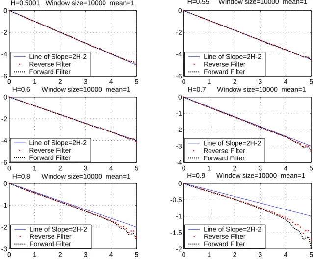
0 0.5 1 1.5 2 2.5 3 −6 −5 −4 −3 −2 −1 0 1 2 3 Log 10(m) Log 10 [C m (0)/C(0)] H=0.75 Ideal H=0.75 Upper−Bound Lower−Bound

Figure 2.4: The lower and the upper bounds of log[Cm(0)/C1(0)].

the nearest integers are therefore necessary. We will numerically examine the impact on self-similarity due to filter truncation and output rounding in later subsections.

2.1.2

Impact On Self-Similarity Due To Filter Truncation

Define h[k; W ] = h[k] · l{0 ≤ k < W }. Then, the impact of the truncation window size.

W on the degree of self-similarity of the filter output process can be characterized through

the derivation of the marginal variance Cm(0; W ) of the respective m-averaged filter output process. Again, we derive Cm(0; W ) through the help of the technique of the variance-equivalent m-average process.

- _{H(w; W )} -. -. -. , X3, X2, X1 . . . , Y3, Y2, Y1 G(w; m) . . . , ¯Y (m) 3 , ¯Y (m) 2 , ¯Y (m) 1 -i.i.d. Poisson

Figure 2.5: The variance-equivalent m-averaged process of the truncated filter output process.

Let G(ω; m) be the transfer function of the filter g[n; m], and let L(ω; W, m)= H(w; W )G(w; m).. Then, `[n; W, m] = n X i=0 g[i; m] × h[n − i; W ] = 1 m min{n,m−1}_X i=max{0,n−W +1} h[n − i].

By letting Sy(w; W ) be the truncated counterpart of Sy(ω), we obtain:

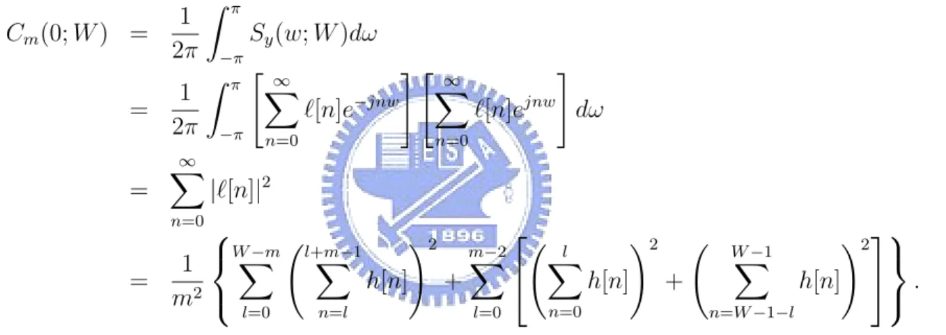
Cm(0; W ) = 1 2π Z _π −π Sy(w; W )dω = 1 2π Z _π −π " _∞ X n=0 `[n]e−jnw # " <sub>∞</sub> X n=0 `[n]ejnw # dω = ∞ X n=0 |`[n]|2 = 1 m2    W −m_X l=0 Ã_l+m−1 X n=l h[n] !2 + m−2_X l=0   Ã _l X n=0 h[n] !2 + Ã _{W −1} X n=W −1−l h[n] !2    . Based on the above formula, we numerically depict log₁₀[Cm(0; W )/C1(0; W )] versus log10(m) in Fig. 2.6, and observe that there are two apparent different self-similar behaviors for differ-ent m values. The resultant degree of self-similarity is close to the target one when m ≤ W , but the slope of the variance-time curve quickly turns to a non-self-similar value, −1, once

m > W .

2.1.3

Impact On Self-Similarity Due To Output Rounding

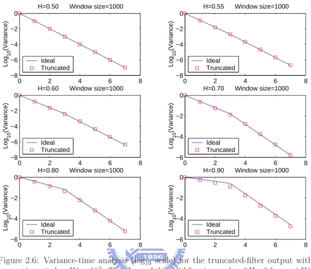
In this subsection, we further empirically examine the output rounding effect on self-similarity. Table 2.1 lists the resultant Hurst parameter of the trace synthesized according to the

sys-0 2 4 6 8 −8 −6 −4 −2 0 Log 10 (Variance) H=0.50 Window size=1000 Ideal Truncated 0 2 4 6 8 −8 −6 −4 −2 0 Log 10 (Variance) H=0.55 Window size=1000 Ideal Truncated 0 2 4 6 8 −8 −6 −4 −2 0 Log 10 (Variance) H=0.60 Window size=1000 Ideal Truncated 0 2 4 6 8 −6 −4 −2 0 Log 10 (Variance) H=0.70 Window size=1000 Ideal Truncated 0 2 4 6 8 −6 −4 −2 0 Log 10 (Variance) H=0.80 Window size=1000 Ideal Truncated 0 2 4 6 8 −6 −4 −2 0 Log 10 (Variance) H=0.90 Window size=1000 Ideal Truncated

Figure 2.6: Variance-time analysis (log₁₀ scale) for the truncated-filter output with truncation window W = 103_{. The slope of the solid line is equal to 2H −2 for m ≤ W ,}

and −1 for m > W .

tem in Fig. 2.7. It indicates that the rounding-to-the-nearest-integer operation on the filter output will have “unstable” impact on the degree of self-similarity of the output trace. Our simulations suggests that such an unstable impact can be neglected if the ratio of the maxi-mal rounding error (i.e., 0.5) against the input mean λ is made less than 5%.

- _{H(w; W )}

-. -. -. , X3, X2, X1 . . . , bY3+ 0.5c, bY2+ 0.5c, bY1+ 0.5c

i.i.d. Poisson A self-similar arrival

Figure 2.7: The proposed asymptotic self-similar traffic synthesizer. H(w; W ) represents a truncated version of H(ω) with truncation window W . The quantity bYi+ 0.5c equals the

closest integer to Yi.

Table 2.1: Comparison between the resultant Hurst parameters of the traces synthesized by the filter-based algorithm and the targeted ideal Hurst parameters.

Window size= 10000 Ideal H V-T(λ = 1) V-T(λ = 10) 0.5001 0.4898783 0.5064982 0.55 0.5504289 0.5344366 0.6 0.6413529 0.5641452 0.7 0.4775099 0.7013537 0.8 0.5399816 0.7799114 0.9 0.5958403 0.8716414

2.2

The Reverse Filter Versus The Forward Filter

It can be easily seen that the z-transforms, X(z) and Y (z), of the filter input and output can be re-characterized by (1 − z−1₎a_{Y (z) = X(z). Again, by Taylor’s expansion,}

(1 − z−1)a= 1 + −a 1! z −1₊−a(1 − a) 2! z −2_{+ · · · = 1 − a} ∞ X n=1 Γ(n − a) Γ(n + 1)Γ(1 − a)z −n_.

Hence, the outputs y[1], y[2], y[3] . . . can be also obtained through an infinite impulse response (IIR) filter as:

y[n] = x[n] + a ∞ X k=1 Γ(k − a) Γ(k + 1)Γ(1 − a)y[n − k] = x[n] + ∞ X k=1 h0_{[k] · y[n − k],} where h0_{[n] =}. a · Γ(n − a) Γ(n + 1)Γ(1 − a) = (H − 0.5) · Γ(n − H + 0.5) Γ(1.5 − H)Γ(n + 1) for k ≥ 1.

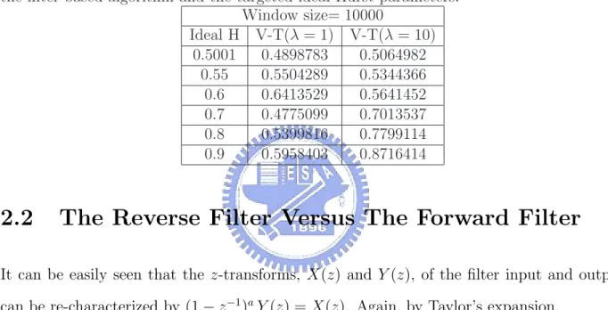
We refer h[·] as the forward filter and h0_{[·] as the reverse filter, since the latter has a} feedback or reverse path. Both h[·] system and h0_{[·] system can generate a true self-similar} process in response to, say, an i.i.d. Poisson input; however, unlike the forward filter, the reverse filter gives an infinite impulse response filter (IIR) even if a finite truncation on

h0_{[·] is applied. This may give a false impression that the reverse system equipped with an} infinite impulse response (IIR) filter of finite number of coefficients can synthesize a more self-similar trace than the forward system with truncated forward filter of the same computational complexity (or more specifically, the same truncation window). Our simulations, however, indicate that the effective range of both filters are actually similar (cf. Fig. 2.8).

2.3

Concluding Remarks

In this chapter, a new model is proposed for the synthesization of self-similar traffics based on the filter technique. The synthesized trace can be made long-range dependent with adjustable levels of bustiness and correlation. Only three parameters need to be specified in our model:

H is the targeted self-similar parameter that controls the bustiness and correlation of the

synthetic traffic, λ defines the mean of the synthesized traffic, and W determines not only the length of the filter (which in turns determines the algorithmic complexity) but also the valid aggregation size of self-similar nature from the aspect of variance-time analysis.

When being compared to the two known self-similar traffic synthesizers—random

mid-point displacement and Paxson’s spectrum fitting, our model provides advantages that the

synthetic traffic can be generated on the fly, and is always non-negative. The algorithmic complexity of Paxon’s spectrum fitting was shown to be less than the random midpoint dis-placement, and is given by (n/2) log₂(n+2), where n is the length of the synthetic trace. The complexity of our model, however, is dependent on W , and is equal to n × W . Hence, when the valid aggregation size of self-similar nature is specified, the complexity of our model only

0 1 2 3 4 5 -6

-4 -2 0

H=0.5001 Window size=10000 mean=1

0 1 2 3 4 5

-6 -4 -2 0

H=0.55 Window size=10000 mean=1

0 1 2 3 4 5

-6 -4 -2 0

H=0.6 Window size=10000 mean=1

0 1 2 3 4 5 -4 -3 -2 -1 0

H=0.7 Window size=10000 mean=1

0 1 2 3 4 5

-3 -2 -1 0

H=0.8 Window size=10000 mean=1

0 1 2 3 4 5 -2 -1.5 -1 -0.5 0

H=0.9 Window size=10000 mean=1 Line of Slope=2H-2 Reverse Filter Forward Filter Line of Slope=2H-2 Reverse Filter Forward Filter Line of Slope=2H-2 Reverse Filter Forward Filter Line of Slope=2H-2 Reverse Filter Forward Filter Line of Slope=2H-2 Reverse Filter Forward Filter Line of Slope=2H-2 Reverse Filter Forward Filter

Figure 2.8: Variance-time plots (log₁₀ scale) for the two filter-based synthetic arrivals with truncation window 104 _{and mean rate 1.}

Chapter 3

Correlation Approximation to the

Mutual Information of Self-Similar

Processes

3.1

Introduction

Mutual information and correlation coefficient are both used as measures of dependance between random sources [27]. Generally speaking, the correlation coefficient only measures the linear dependance, while mutual information can represent the general dependance [28]. Thus, in the sense of generality, mutual information is a somewhat better quantity to measure the dependance than the correlation coefficient. However, estimating the mutual information function is much more difficult than estimating the correlation coefficient, as it requires a complete knowledge about the distributions.

In this chapter, we focus on the following question: Given the correlation coefficients of random sources, what is the minimum possible value of mutual information? An upper bound and a lower bound of this minimum possible value were established in situation where the correlation coefficients are small. It was subsequently shown that both bounds can be approximated by half the square of the correlation coefficient when the two random sources are both one dimensional. When the random sources are multidimensional, we found that

this minimum mutual information function can be approximated by half the square of the Frobenius norm of the cross correlation coefficient matrix. We also address some examples to show the accuracy of these approximative bounds.

3.2

Definitions and Notations

Definition 3.1. Given two random sources X and Y (not necessarily random variables or random vectors), the mutual information function is defined as:

I (PX,Y) or I(X; Y ) =4 X x,y PX,Y(x, y) log PX,Y(x, y) Ã X z PX,Y(z, y) ! Ã X w PX,Y(x, w) !,

where PX,Y(x, y) is the probability of the event (X, Y ) = (x, y).

Definition 3.2. The divergence function of PX against QX is defined as:

D (PXkQX) =4 X x PX(x) log PX(x) QX(x) ,

where PX(x) and QX(x) are two probability mass functions, and the support of PX is con-tained in the support of QX.

A straightforward consequence of the above definitions is that:

I (PX,Y) = D (PX,YkPX × PY) , where PX(x)=4

P

wPX,Y(x, w) and PY(y) 4

= P_zPX,Y(z, y).

Definition 3.3. (Minimum mutual information of a probability set) The minimum mutual information function with respect to a set S of probabilities is defined as:

Imin(S)

4 = min

PX,Y∈S

I (PX,Y) ,

Definition 3.4. (Minimum divergence function of a probability set and two marginal distributions) The minimum divergence function with respect to a set S of probabilities and two marginal distributions, PX and PY, is defined as:

Dmin(S, PX, PY) 4 = min

QX,Y∈S

D (QX,YkPX × PY) ,

where QX,Y is the probability mass function of X and Y chosen from the set S.

Definition 3.5. (Correlation coefficient matrix) Given two random vectors, ~X =

(X1, ..., Xn) and ~Y = (Y1, ..., Ym), the (i, j)-component of the correlation coefficient matrix of ~X and ~Y is defined as:

C_X,~~ _Y(i, j) = E[ ˆ4 XiYˆj],

where ( ˆX1, ..., ˆXn) is the Karhunen-Loeve transformation of ~X, and each of ( ˆX1, ..., ˆXn) has zero mean and unity variance and is uncorrelated to the others, and ( ˆY1, ..., ˆYn) is defined similarly with respect to ~Y .

Since Karhunen-Loeve transformation is invertible,

I (X1, ..., Xn; Y1, ..., Ym) = I( ˆX1, ..., ˆXn; ˆY1, ..., ˆYn).

To simplify the proof in later section, we will assume that the considered ~X and ~Y are

already their Karhunen-Loeve transformation counterparts that satisfy the conditions of uncorrelatedness, zero-mean and unity variance.

Definition 3.6. (Frobenius norm) The Frobenius norm of a matrix C is defined as:

kCk =4 Ã X i,j C2(i, j) !_1/2 ,

3.3

Main Theorems

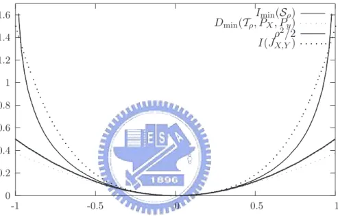
Theorem 3.1. For two bounded1 _{random variables X and Y respectively with marginal} distributions PX and PY, Imin(Sρ) = ρ2 2 + o(ρ 2_{), as ρ → 0,} where

Sρ = {Q4 X,Y : QX = PX, QY = PY and EQ[XY ] = ρ},

QX and QY are the marginal distributions of QX,Y, EQ[·] denotes that the expectation value is calculated according to distribution QX,Y, and o(·) is the little-o notation [29, pp. 286].

Note that Sρ= Sρ(PX, PY) is actually a function of the marginal distributions of PX and

PY. For convenience, we drop “(PX, PY)” in the notation, and reserve PX and PY to always denote given marginals.

It can be shown that Imin(Sρ) is a convex function of ρ [26]. Specifically,

Imin ¡ Sλρ1+(1−λ)ρ2 ¢ ≤ Imin(λSρ1 + (1 − λ)Sρ2) = Dmin(λSρ1 + (1 − λ)Sρ2, PX, PY) = min Q(1)_X,Y∈Sρ1 Q(2)_X,Y∈Sρ2 D ³ λQ(1)_X,Y + (1 − λ)Q(2)_X,Y ° ° ° PX × PY ´ ≤ min Q(1)_X,Y∈S_ρ1,Q(2)_X,Y∈S_ρ2 h λD ³ Q(1)_X,Y ° ° ° PX × PY ´ +(1 − λ)D³Q(2)_X,Y ° ° ° PX × PY ´i = λImin(Sρ1) + (1 − λ)Imin(Sρ2) .

We now proceed to prove the theorem.

1 _{By ”boundedness”, we mean that there exists B > 0 such that P}

X[x ∈ < : |x| < B] = PY [y ∈ < : |y| < B] = 1.

Proof. In this proof, we first find a lower bound of Imin(Sρ). Then we use a specific distribu-tion contained in Sρ to form an upper bound of Imin(Sρ). The theorem is then proved since both bounds have the form ρ2_{/2 + o(ρ}2_{) as ρ → 0.}

Define a set Tρ as: Tρ 4

= {QX,Y : EQ[XY ] = ρ}. From the standpoint of mutual in-formation and Karhunen-Loeve transin-formation, we can assume without loss of generality that both PX and PY have zero marginal mean and unity marginal variance, and they are uncorrelated.

Since Sρ ⊂ Tρ, Imin(Sρ) = Dmin(Sρ, PX, PY) ≥ Dmin(Tρ, PX, PY). Now, we apply the Lagrange multiplier method to evaluate Dmin(Tρ, PX, PY), i.e., to minimize

F (QX,Y) = D (QX,YkPX × PY) − β Ã X x,y xyQX,Y(x, y) − ρ ! − θ Ã X x,y QX,Y(x, y) − 1 ! ,

subject to the following restrictive conditions: X x,y xyQX,Y(x, y) = ρ, (3.1) and X x,y QX,Y(x, y) = 1.

We then take the derivative of F (QX,Y) with respect to QX,Y(x, y), and obtain

∂F (QX,Y)

∂QX,Y(x, y)

= 1 + log QX,Y(x, y)

PX(x)PY(y)

− βxy − θ.

Letting the above derivative be zero, we have that the optimal QX,Y must satisfy:

QX,Y(x, y) =

PX(x)PY(y) exp{βxy} P

u,vPX(u)PY(v) exp{βuv}

= PX(x)PY(y) exp{βxy} M(β) , where M (β) =X u,v PX(u)PY(v) exp{βuv}.

Taking the above result into Dmin(Tρ, PX, PY) yields

Dmin(Tρ, PX, PY) = βρ − C (β) ,

where C (β) = log M (β). Denote f (β) = ∂C(β)/∂β, and observe that

f (β) =X

x,y

xyQX,Y(x, y) = EQ[XY ]. Hence, the restrictive condition in (3.1) can be written as f (β) = ρ.

Since X and Y are bounded with respect to distributions PX and PY, respectively, the moment generating function M(β) is defined throughout an interval (−β0, β0) for some β0 > 0, which implies that moments of all orders are finite (namely, P_x,yxi_yj_P

X(x) PY(y) < ∞ for i ≥ 1 and j ≥ 1), and M(β) has a Taylor expansion about origin with positive radius of convergence [30, pp. 278], and so do C(β) and f (β). Using the Taylor expansions of f (β) and C (β), we have f (β) = f (0) + f0_{(0)β +} f00(0) 2! β 2_{+ o(β}2₎ = β + γ 2β 2_{+ o(β}2_), and C (β) = C(0) + C0_{(0)β +} C00(0) 2! β 2₊C000(0) 3! β 3_{+ o(β}3₎ = β2 2 + γ 6β 3_{+ o(β}3_), where γ = P_x,yx3_y3_P

X(x)PY(y). Accordingly, β = ρ + o(ρ2), and C (β) = ρ2/2 + o(ρ3). This immediately concludes Dmin(Tρ, PX, PY) = βρ − C (β) = ρ2/2 + o(ρ3).

Now, we turn to the task of finding an upper bound. It suffices to use a trial distribution in Sρ to form an upper bound. Define this trial distribution as:

JX,Y(x, y) 4

and examine2 _thatP

x,yJX,Y(x, y) = 1, P

yJX,Y(x, y) = PX(x), P

xJX,Y(x, y) = PY(y), and P

x,yxyJX,Y(x, y) = ρ. Using the inequality

x −x2 2 + x3 3 ≥ log (1 + x), for |x| < 1, we have I (JX,Y) = X x,y

PX(x)PY(y)(1 + ρxy) log(1 + ρxy)

≤ ρ 2 2 − γ 6ρ 3₊ η 3ρ 4_, where η =P_x,yx4_y4_P

X(x)PY(y). Since I (JX,Y) ≥ Imin(Sρ) ≥ Dmin(Tρ, PX, PY), we have

Imin(Sρ) =

ρ2 2 + o(ρ

2_).

Theorem 3.2. Consider two bounded random vectors ~X = (X1, ..., Xn) and ~Y = (Y1, ..., Ym). If the correlation coefficient matrix C satisfies |C(i, j)| < ρ for each 1 ≤ i ≤ n and 1 ≤ j ≤ m, then Imin(SC) = 1 2kCk 2_{+ o(ρ}2_{), as ρ → 0,} where SC 4 = {Q_X,~~ _Y : Q_X~ = P_X~, Q_Y~ = P_Y~ and EQ[XiYj] = C(i, j)},

Q_X~ and Q_Y~ are the marginal distributions of Q_X,~~ _Y, EQ[·] denotes that the expectation value is calculated according to distribution Q_X,~~ _Y, and o(·) is the little-o notation [29, pp. 286].

Proof. The proof is similar to the previous theorem; hence, it is omitted. 2_{Notably, following footnote 1, we can guarantee that 0 ≤ J}

3.4

Examples

To discuss the accuracy of the upper and lower bounds of the minimum mutual information function, we first consider the simple case that both random variables X and Y are binary random variables, each taking values from {0, 1}. In this case, given the correlation coefficient

ρ and marginal mean, a = E[X] and b = E[Y ], one can determine the joint distribution of X and Y , i.e.,

PX,Y(0, 0) = (1 − a)(1 − b) + r

PX,Y(0, 1) = (1 − a)b − r

PX,Y(1, 0) = a(1 − b) − r

PX,Y(1, 1) = ab + r

where r = E[XY ] − E[X]E[Y ] = ρ[a(1 − a)b(1 − b)]1/2_{. The mutual information I(X; Y )} can be written as I(X; Y ) = Hb(b) − aHb ³ b + r a ´ − (1 − a)Hb µ 1 − b + r 1 − a ¶ ,

where Hb(b) = −b log (b) − (1 − b) log (1 − b) is the binary entropy function. Thus, in binary case, Imin(Sρ) = I(X; Y ). We then take the uniform marginal distributions as an example, i.e., a = 1

2 and b = 12, and obtain Dmin(Tρ, PX, PY) = ρ tanh

−1_{(ρ) +}1

2log (1 − ρ2) = I(X; Y ). Therefore, the lower bound used in the proof coincides with the minimum mutual information function. Notably, the simple binary case has already been examined in [28].

A good example that meets the boundedness assumption of our theorem is the Morgen-stern distribution [31] that has the density of

p(x, y) = 1 + α(2x + 1)(2y + 1),

information with respect to the correlation coefficient can be obtained easily as: I(X; Y ) = α2 18 + α4 300 + o(α 5_{) =} ρ2 2 + o(ρ 2_).

An example that can be used to show that Imin(Sρ) is indeed a lower bound to the mutual information of PX,Y ∈ Sρ is the bivariate density p(x, y) = pY |X(y|x)pX(x), where pX(x) =

1

2a · l[|X| ≤ a] and pY |X(y|x) = 2b1 · l[|Y − αX| ≤ b], which exactly define a uniform diagonal strip. The asymptotic mutual information of the uniform diagonal strip can be derived easily

from [31] as |ρ|₂ −|ρ|₄3 + o(|ρ|4_{). This indicates that in some situations, I(X; Y ) > I}

min(Sρ). The validity of the theorem statement can be extended to the (unbounded) case that

PX and PY are both Gaussian distributed. In this case, the minimum value of mutual information can be achieved by a jointly Gaussian distributed QX,Y. One can derive that for Gaussian PX and PY, Imin(Sρ) = −1₂log (1 − ρ2). The lower bound, however, is given by:

Dmin(Tρ, PX, PY) = − 1 2+ µ 1 4 + ρ 2 ¶1 2 + 1 2log à −1 2 + (14 + ρ2) 1 2 ρ2 ! ,

and is smaller than the simple hyperbolic approximation of Imin(Sρ) ≈ ρ 2

2. In addition, the “upper bound” used in the proof ρ₂2 + ρ4 _{may become smaller than I}

min(Sρ) at large |ρ|. Since we only use the upper bound under |ρ| ¿ 1, we would not expect it to be useful outside the concerned range.

0 0.2 0.4 0.6 0.8 1 1.2 1.4 1.6 -1 -0.5 0 0.5 1 I_min(S_ρ) Dmin(Tρ, PX, Py) ρ2_/2 I(JX,Y)

Figure 3.1: The bounds and minimum mutual information for Gaussian distributed PX and

Chapter 4

Bayesian Decentralized Detection for

Exponential Distributions

A decentralized detection system consists of n sensors, sometimes geographically dispersed, and a remote fusion center. Each of the sensor observes a phenomenon (often modeled as a random variable Xi), summarizes it into a single bit ui, and then transmits ui to the fusion center uncooperatively. Based on received {ui}ni=1, the fusion center determines whether

{Xi}ni=1are drawn from the null distribution P (·|H0) or the alternative distribution P (·|H1). Decentralized detection, despite that it has a simple scenario, and has been studied extensively for more than two decades, still has many unsolved issues in the fundamental level. One of these unsolved issues concerns the global optimal strategy for the design of sensors and the fusion center. The difficulties comes from several points. Firstly, only the necessary conditions for the optimal strategy are known; hence, one have to search all the solutions to the equations of the necessary conditions in order to determine the global optimum. Moreover, these equations are coupled and nonlinear, and hence, to solve them is proved to be a hard mission [32]. The knowledge about the global optimal strategy is so little that there are almost no analytical results for the system with more than two sensors. The asymptotic results, however, had been found more pleasantly: the system with identical

sensors has the same exponents of error probabilities as the optimal system [37]; the ratio of error probabilities between these two systems are shown bounded from above and from below [36]. Yet the exact and analytical results for the system with some finite n > 2 are still absent, although such results will give us more insight about the global optimum than the asymptotic results.

In this chapter, we analyze the decentralized classification problem for exponential sources for n > 2, and validate an intuition that the optimal system is the system with identical sensors. To our knowledge, there is no similar analytical result for the global optimum for the system with more than two sensors.

4.1

Preliminaries

Definition 4.1. If X is a random variable with an exponential distribution, then the prob-ability that X is greater than some number x is given by

1 − FX(x) = Pr(X > x) = e−αx

for x ≥ 0, where α is a positive parameter, and FX(x) is the cumulative distribution function (CDF) of X.

It follows that the probability density function (PDF) of an exponential distribution has the form

fX(x) = αe−αx, for x ≥ 0.

In this chapter, we concern the following binary hypothesis testing problem for exponen-tial distributions:

versus H0 : gX(xi) = γe−γxi, or equivalently, H1 : FX(xi) = 1 − e−βxi versus H0 : GX(xi) = 1 − e−γxi,

for i = 1, 2, . . . , n, β < γ, and for xi ≥ 0, where xi is the observed value of the random variable Xi at the i-th sensor. We assume that {Xi}ni=1 form a set of independent and identically distributed (i.i.d.) random variables. The prior probabilities of H1 and H0 are denoted as r1 and r0 or simply r and 1 − r, respectively. For a fixed fusion rule, it is known that the optimal local decision rule for each sensor is the local likelihood ratio test (LLRT), i.e., fX(xi) gX(xi) = βe−βxi γe−γxi ui=1 R ui=0 λi or equivalently, xi ui=1 R ui=0 ti

for i = 1, 2, . . . , n, where ui is the decision of i-th sensor, ti = _γ−β1 log(λ_ξi) is some constant threshold to be decided, and ξ = β_γ. Let PD(λi) and PF(λi) denote respectively the detection probability and the false alarm probability for the i-th sensor, where

PD(λi) = Prob(ui = 1|H1) = 1 ˜ λi ˜ β and PF(λi) = Prob(ui = 1|H0) = 1 ˜ λi ˜ γ.

Both are functions of the LLRT threshold λi as ˜λi = λ_ξi, ˜β = _γ−ββ and ˜γ = _γ−βγ . Notably, 1 ≤ ˆλ ≤ ∞, ˆγ = ˆβ + 1 and dPD

PF, i.e., PD(PF(i)) = PF(i)ξ and λi = dPD(PF(i)) dPF(i) = ξPD(PF(i)) PF(i) ,

where we abuse the notations to let PF(i) and PD(PF(i)) represent the false alarm probability and the detection probability of the i-th sensor, respectively. The graph consists of all (PF, PD) pairs is referred to as Receiver Operating Characteristics (ROC curve), which is identical for all sensors since the statistics of their observations are all the same.

The sensors transmit their decisions {ui}ni=1 to the fusion center that makes the final decision u0, which equals ` when the fusion center favors H`. Once the fusion rule is fixed, we can then evaluate the system detection probability QD(λ1, · · · , λn) = Prob(u0 = 1|H1), the system false alarm probability QF(λ1, · · · , λn) = Prob(u0 = 1|H0) and the probability of error Pe(n)(λ1, · · · , λn) = r(1 − QD(λ1, · · · , λn)) + (1 − r)QF(λ1, · · · , λn) as functions of the local thresholds λ1, · · · , λn.

It is known from classical detection theory that the fusion center should make the overall decision u0 based on the likelihood ratio test of received u1, , u2. . . , un. Therefore, the error probability can be expressed as

P_e(n)(λ1, · · · , λn) = X un_∈{0,1}n min " r à 1 − n Y i=1 PD(λi)ui(1 − PD(λi))1−ui ! , (1 − r) n Y i=1 PF(λi)ui(1 − PF(λi))1−ui # .

The above formula, however, is in general not differentiable, and could give us little insight into the optimal choice of LLRT thresholds (λ1, · · · , λn).