設計高效能之頻繁封閉項目集維護演算法

全文

(1)國立交通大學資訊科學系碩士論文. 設計高效能之頻繁封閉項目集維護演算法 Designing Efficient Mining algorithms for Frequent Closed Itemsets Maintenances. 研究生：邱成樑指導教授：曾憲雄. 博士. 中華民國九十四年六月 I.

(2) 設計高效能之頻繁封閉項目集維護演算法 Designing Efficient Mining algorithms for Frequent Closed Itemsets Maintenances. 研究生：邱成樑. Student：Cheng-Liang Chiu. 指導教授：曾憲雄. Advisor：Shian-Shyong Tseng. 國立交通大學資訊科學系碩士論文. A Thesis Submitted to Institute of Computer and Information Science College of Electrical Engineering and Computer Science National Chiao Tung University in partial Fulfillment of the Requirements for the Degree of Master in Computer and Information Science June 2005 Hsinchu, Taiwan, Republic of China. 中華民國九十四年六月 II.

(3) 設計高效能之頻繁封閉項目集維護演算法. 研究生:邱成樑. 指導教授:曾憲雄博士. 國立交通大學資訊科學研究所. 摘要如何從龐大且複雜的資料庫中萃取出有用的知識與資料是近來非常熱門的研究課題。在真實生活中，新資料的加入使得資料探勘的結果不斷改變。當新的資料新增時為了避免重新處理整個資料庫來獲得新的探勘結果；一些漸進式的資料探勘演算法利用儲存之前的探勘結果來降低新增資料時所需要處理的時間。然而，傳統的漸進式資料探勘技術遇到頻繁項目集(Frequent Itemsets)長度很長時，大量頻繁項目集的保存將使得漸進式資料探勘有實做上的困難。此外，傳統的漸進式資料探勘技術每次都必須消耗額外的存取動作重新掃描一次資料庫以確定是否有新的頻繁項目集產生。有鑑於此，此篇論文將封閉項目集(Closed Itemsets)與準大項目集(Pre-large Itemsets)的概念導入到漸進式資料探勘；封閉項目集的概念是在沒有遺失任何資訊的情況下將資料進行壓縮，透過此優點來將漸進式資料探勘預先保存的資料進行壓縮。而準大項目集則是用一種緩衝區的概念來避免項目集直接從有效項目集被判定為無效項目集，且反之亦然；這樣可避免常對資料庫進行重新掃描。基於這兩個概念，我們提出封閉項目集維護演算法(CIM)與準大封閉項目集維護演算法(CIM-P)兩個新的漸進式資料探勘演算法，CIM 利用封閉項目集來有效取得探勘結果，減少維護於記憶體中的項目集。而 CIM-P 則利用緩衝區來降低 CIM 在每次加入新資料時，必須重新掃描資料庫的機率。關鍵字:封閉項目集、漸進式資料探勘、關聯式規則、資料探勘 III.

(4) Designing Efficient Mining algorithms for Frequent Closed Itemsets Maintenances. Student: Cheng-Liang Chiu. Advisor: Dr. Shian-Shyong Tseng. Department of Computer and Information Science National Chiao Tung University. Abstract Recently, mining association rules from transaction databases has been one of the most interesting and popular research topics in data mining. In real-world applications, a database grows over time such that existing association rules may become invalid or new implicitly valid association rules may appear. Some researchers have thus developed incremental mining algorithms to maintain association rules without re-processing the entire database whenever the database is updated. The common idea among these approaches is to store previously mined itemsets in advance for later use. However, for a dense database, the performance of classical incremental mining algorithms will degrade dramatically due to a huge amount of pre-stored mining information. On the other hand, most incremental mining algorithms are required one scan of original database to discover new implicitly valid rules. When the original database is massive, this will result in excessive I/O cost. In this study, we attempt to utilize the concepts of closed itemsets and pre-large itemsets dealing with the two challenges, respectively. The closed itemsets can losslessly determine all the pre-stored mined itemsets and their exact support, but are orders of magnitude smaller than all pre-stored patterns. The pre-large patterns act as a buffer to avoid the movements of itemsets directly from valid to invalid and vice-versa when the database maintained. Based on the two concepts, two novel incremental mining algorithms called Closed Itemsets Maintenance (CIM) and CIM with Pre-large concept (CIM-P) are thus developed to efficiently maintain association rules, especially in a dense database. Keywords: closed itemsets, incremental mining, association rules, data mining. IV.

(5) 致謝. 能順利的完成此篇論文，首先最先要感謝的是我的指導教授，曾憲雄博士，曾教授在我碩士班的兩年期間相當耐心的指導我的論文研究；從他身上學習到許多領導處世的技巧，寶貴的經驗讓我獲益匪淺，不甚感激。同時也感謝我的口試委員，洪宗貝教授，曾秋蓉教授以及彭文志教授所給予的寶貴意見；讓我的論文研究能夠更有價值。. 接下來要感謝王慶堯學長，兩年期間讓我學會許多理論知識及實務技巧，也給予我許多對於此篇論文的寶貴意見，協助我論文上的修改工作；並常與我一起研究到深夜而無法休息，讓這篇論文能夠順利的完成。。. 此外必須謝實驗室學長平日的諸多協助，特別是林順傑學長與曲衍旭學長。同時也感謝實驗室同窗夥伴，黃柏智、吳政霖、李育松、陳瑞言、陳君翰、宋昱璋、林易虹等人在生活上和課業上的協助，大家互相扶持的渡過這段忙碌且充實的碩士生涯。. 另外要感謝我的母親在背後默默支持我完成我的碩士生涯。最後要感謝我的妻子，在這兩年的碩士生的求學過程中做我背後無聲卻最有力的支柱；讓我能在這兩年無後顧之憂的完成我的學業，讓我的心中充滿感謝。. 要感謝的人很多，無法一一詳述，在此僅向所有幫助過我的人，致上我最深的謝意。. V.

(6) Table of contents 摘要..............................................................................................................................III Abstract ........................................................................................................................IV 致謝...............................................................................................................................V Table of contents ..........................................................................................................VI Chapter 1: Introduction ..................................................................................................1 Chapter 2: Related Work................................................................................................4 2.1 Closed itemsets mining approaches .................................................................4 2.2 Incremental mining approaches .......................................................................5 Chapter 3: Preliminary Concepts ...................................................................................9 Chapter 4: Frequent Closed Itemsets Maintenance .....................................................12 4.1 Joint closed itemsets ......................................................................................12 4.2 The effect of intersectional closed itemsets ...................................................14 Chapter 5: The CIM Algorithm....................................................................................17 5.1 The closed maintenance tree (CMT)..............................................................18 5.2 Generation of the CO set................................................................................19 5.3 Generation of the CP set ................................................................................23 Chapter 6: The CIM Algorithm with Pre-large Concept: CIM-P Algorithm ...............27 6.1 The concept of pre-large closed itemsets.......................................................27 6.2 The detail Algorithm of CIM-P......................................................................31 Chapter 7: Experiments................................................................................................33 7.1. The experimental environment and the datasets used...................................33 Chapter 8: Conclusion..................................................................................................38 Reference .....................................................................................................................40. VI.

(7) Chapter 1: Introduction Data mining technology has become increasingly important in the field of large databases and data warehouses. This technology helps discover non-trivial, implicit, previously unknown and potentially useful knowledge, thus being able to aid managers in making good decision. Among various types of databases and mined knowledge, mining association rules from transaction databases is the most interesting and popular. In general, the process of mining association rules can roughly be decomposed into two tasks: finding frequent itemsets satisfying the user-specified minimum support threshold from a given database and generating interesting association rules satisfying the user-specified minimum confidence threshold from found frequent itemsets. Since the first task is very time-consuming when compared to the second one, the major challenges in mining association rules thus focus on how to reduce the search space and decrease the computation time in the first task. Some famous mining approaches, such as Apriori [4], DIC [10], DHP [29], Partition [31], Sampling [26], GSP [5] and FP-Growth [20][33], have been proposed.. In real-world applications, a database grows over time such that existing association rules may become invalid or new implicitly valid association rules may appear. Recently, some researchers have developed incremental mining algorithms to maintain association rules without re-processing the entire updated database [13]. The common idea of these researches lies in that, the previously mined information such as mined frequent itemsets are stored in advance; when new transactions are inserted, (a) a large portion of candidate itemsets can be decided using the pre-stored mined frequent itemsets; (b) only a small portion of candidate itemsets obtained from the new transactions without sufficient information needs to be re-processed against the 1.

(8) original database. Task (a) is responsible for updating previously mined association rules, and Task (b) is responsible for finding new association rules. Much computation time can thus be saved in this way. However, for a dense database such as census data and DNA sequences, the computation cost of Task (a) will be getting tremendous due to a huge amount of previously mined frequent itemsets. For example, a frequent 30-itemset (a frequent itemset consisting of 30 items) implies the presence of 230-2 additional frequent itemsets as well. The performance of classical incremental mining algorithms will degrade dramatically. On the other hand, most incremental mining algorithms are required one scan of original database to deal with Task (b). When the original database is massive, this will result in excessive I/O cost. As a result, in this study, we attempt to utilize the concepts of closed itemsets and pre-large itemsets to overcome the two challenges, respectively.. In a dense database, many itemsets usually appear together, and we can consider them together. The concept of closed itemsets, which is denoted as the itemsets having no proper superset with the same support, can be treated as a lossless compression for all itemsets in the database. It can also reduce redundant rules generated [34]. Therefore, using the set of frequent closed itemsets instead of the set of frequent itemsets from the original database as the pre-stored mining information can increase both efficiency and effectiveness of an incremental mining algorithm. The set of frequent closed itemsets can easily determine all the frequent itemsets and their exact supports, and its order of magnitude is smaller than the set of all frequent itemsets.. In general, the number of newly inserted transactions is much smaller than the number of records in the original database. Only the candidate itemsets whose. 2.

(9) supports are slightly less than the minimum support in the original database are possible to be frequent after database maintenance. The concept of pre-large itemsets is denoted as the set of itemsets having support between a lower support threshold, which is smaller than the given minimum support, and an upper support threshold, which is equal to the given minimum support. Therefore, using the pre-large closed itemsets to enlarge the amount of pre-stored frequent closed itemsets can reduce the cost of re-processing the entire database at the expense of storage spaces. This is because they act as a buffer to avoid the movements of closed itemset directly from infrequent to frequent and vice-versa during the incremental mining process.. Although using the concept of closed itemsets can effectively reduce the number of itemsets considered, some closed itemsets for the updated database, called joint closed itemsets in this paper, may not be considered by a classical incremental mining algorithm. The major reason is that the set of joint closed itemsets, which was compressed before, cannot be determined by above-mentioned Tasks (a) and (b). In this paper, we thus propose a novel incremental mining algorithm called Closed Itemsets Maintaining (CIM) to extend Tasks (a) and (b) that can efficiently find all frequent closed itemsets for the updated database. Task (a) of CIM algorithm is responsible for extracting the joint closed itemsets, which was compressed by the pre-stored frequent closed itemsets in the original database, and updating them against the newly inserted transactions. Task (b) of CIM algorithm is responsible for generating the candidate itemsets for the updated database which has not been determined in Task (a). Furthermore, based on the concept of pre-large itemsets, we propose the CIM-P algorithm to reduce the cost of Task (b) in the CIM algorithm. Also, we design the bucketing strategy to improve the utility of buffer. The consumption of buffer can be rigidly calculated using the maximum value of buckets. 3.

(10) Chapter 2: Related Work In the following, the previous related studies of closed itemsets mining and incremental mining approaches will be briefly described.. 2.1 Closed itemsets mining approaches. The major challenge in mining association rules is to reduce the search space and decrease the computation time required for mining frequent itemsets. The Apriori algorithm, which is the most well-known, utilizes a level-wise candidate generation approach to reduce its search space such that only frequent itemsets found in the previous level are treated as seeds for generating candidate itemsets in the current level. Many later algorithms [10][29][31][26][5] were based on this property and attempted to further reduce candidate itemsets and I/O costs. However, this Apriori property can not work well for dense databases, such as census data and DNA sequences, or a low minimum support. This is because most generated candidate itemsets are frequent itemsets such that the number of frequent itemsets will grow up exponentially; the performance of an Apriori-like algorithm thus degrades dramatically.. Some researchers have then developed closed itemsets mining algorithms to reduce the number of itemsets generated. Examples include A-close [34], CLOSET [35], CLOSET+ [36] and CHARM [36]. The A-close algorithm is an Apriori-like algorithm using a breadth-first search manner to find frequent closed itemsets directly. However, breadth-first searches may encounter difficulties since there could be many candidates generated and need to scan the database many times. The CLOSET 4.

(11) algorithm [35], an extension of the FP-growth algorithm, uses a depth-first search (recursive divide-and-conquer) manner and a database-projection approach to mine long patterns from the FP-tree (frequent pattern tree) structure representing all transactions of database. However, the CLOSET algorithm may suffer from a sparse database or a low minimum support. An enhancement of the CLOSET algorithm, the CLOEST+ algorithm, thus combines various known search manners and closure-testing strategies to improve the performance of CLOSET. The CHARM algorithm uses a dual itemsets-tidset search tree and the Diffset technique to enumerate closed itemsets from a vertical-layout database. In many dense datasets, the CHARM algorithm has better performance than the A-close, CLOSET and CLOSET+ algorithms.. 2.2 Incremental mining approaches. In real-world applications, a database grows over time such that existing association rules may become invalid or new implicitly valid rules may appear. In these situations, conventional batch-mining algorithms do not utilize previously mined patterns for later maintenance, and may require considerable computation time to re-process the entire updated database to get all up-to-date association rules. Some researchers have developed incremental mining algorithms to maintain association rules without re-processing the entire database whenever the database is updated. Examples include the FUP-based algorithms [13][14], an adaptive algorithm [30], an incremental mining algorithm based on the concept of pre-large itemsets [22], and an incremental updating technique based on the concept of negative border [16][32]. The common idea of these researches lies in that, the previously mined information such as mined frequent itemsets are stored in advance; when new transactions are inserted, 5.

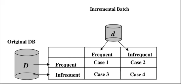
(12) a large portion of candidate itemsets can be decided by using the pre-stored frequent itemsets; only a small portion of candidate itemsets obtained from the new transactions needs to be re-processed against the original database. Much computation time can thus be saved in this way. The correctness of this idea is simply illustrated as follows. Considering an original database and the newly inserted transactions, there are four cases of candidate itemsets shown in Figure 2-1 may arise: Case 1: A candidate itemset is frequent in both the original database and the newly inserted transactions. Case 2: A candidate itemset is frequent in the original database but infrequent in the newly inserted transactions. Case 3: A candidate itemset is infrequent in the original database but frequent in the newly inserted transactions. Case 4: A candidate itemset is infrequent in both the original database and the newly inserted transactions.. Incremental Batch. d Original DB. D. Frequent. Frequent Case 1 Case 3. Infrequent. Infrequent Case 2 Case 4. Figure 2-1: Four cases of candidate itemsets when adding new transactions to existing databases.. 6.

(13) Among the cases, since candidate itemsets in Case 1 are large in both the original database and the new transactions, they are still large after the weighted average of the supports; similarly, candidate itemsets in Case 4 are still small after the new transactions are inserted. Cases 1 and 4 will not affect the final association rules; Case 2 may remove existing association rules; and Case 3 may generate new association rules.. Cheung and his co-workers proposed an incremental mining algorithm, called FUP (Fast UPdate algorithm) [13][14], to efficiently cope with these four cases by pre-storing the previously mined frequent itemsets from the original database. It handles Cases 1, 2 and 4 by updating the pre-stored frequent itemsets against the newly inserted transactions, and re-processes only the itemsets without sufficient information in Case 3 against the original database if necessary.. The performance of the FUP algorithm will get degraded if a lot of candidate itemsets from the newly inserted transactions belong to Case 3. For example, suppose {A}, {B} and {AB} are all the previously mined frequent itemsets from the original database and {C}, {D} and {CD} are the three candidate itemsets from some newly inserted transactions. The final results can not be determined without re-processing the original database.. As a result, Thomas et al. [32] and Feldman et al. [16] utilized the concept of negative border [16] to enlarge the amount of pre-stored mining information in the FUP algorithm for improving the maintenance performance. A negative border of frequent itemsets can be easily formed by excluding the set of frequent itemsets from the set of candidate itemsets generated level by level. In other words, the negative 7.

(14) border consists of the itemsets which are candidates but do not have enough supports. The processing time for Case 3 in the FUP algorithm can be reduced by additionally keeping the negative border of frequent itemsets. Similarly, Hong et al. [22] proposed the concept of pre-large itemsets [22] to enlarge the amount of pre-stored mining information for improving the maintenance performance. The proposed algorithm doesn't need to rescan the original database until a number of new transactions have been inserted.. 8.

(15) Chapter 3: Preliminary Concepts Let I = {i1, i2, …, im} be a set of m items. A subset X of I consisting of k items is called a k-itemset. Let D be a transactional database (TDB) consisting of a set of transactions, where each transaction T consisting of a set of items of I is associated with an identifier called TID, and |D| denotes the number of transactions in D. A transaction T is said to contain X if and only if X ⊆ T. The support of an itemset X, X.sup, in D is denoted as the percentage of transactions in D which contain X. For the itemsets in D, X is called a closed itemset if there does not exist an itemset Y which closes (absorbs) X, where an itemset Y is said to close (absorb) X iff X ⊆ Y and X.sup = Y.sup. CI denotes the set of all closed itemsets in D. Furthermore, if there is no superset of X existing in D, X is also called a maximum itemset.. An association rule is an implication of the form X ⇒ Y, where X and Y are subset of I, and X∩Y = φ. The support of a rule X ⇒ Y, (X∪Y).sup, in D is denoted as the percentage of transactions in D which contain X∪Y, and the confidence of X ⇒ Y is computed by (X∪Y).sup/X.sup. Given the user-specified minimum support threshold, minsup, and minimum confidence threshold, minconf, the problem of mining association rules is to find out all association rules in D that have support and confidence larger than minsup and minconf, respectively. With respect to the minsup, the set of frequent itemset, FI, includes all the itemsets whose support is larger than minsup; the set of infrequent itemset, NI, includes all the itemsets whose support is less than minsup; the set of frequent closed itemset, FCI, includes all the closed itemsets whose support is larger than minsup, FCI = {x|x ∈ CI, x.sup ≥ minsup}; and the set of infrequent closed itemset, NCI, includes all the closed itemsets whose support is less than minsup, NCI = {x| x ∈ CI – FCI}. Note that FCI includes no 9.

(16) itemset which has a superset with the same support, and thus FCI ⊆ FI. The problem of mining association rules can be reduced to the problem of finding FI or FCI in D.. Let d be an increment of new transactions which is added to the original database D, |d| be the number of transactions in d, D+ be the updated database which denotes D ∪ d, and |D+| be the number of transactions in D ∪ d. Therefore, FID, FId and CI D+ denote the FI obtained from D, d and D+ with respect to the same minsup, respectively, and FCI, NI, NFCI or CI obtained from D, d and D+ can have similar meanings. The problem of maintaining association rules is to find FID+ or FCID+. Let the set of original frequent itemsets, O, be defined as O = {x|x ∈ FID}, and the set of potential frequent itemsets, P, be defined as P = {x|x ∈ FId − FID}. By definition, an itemset X ∈ FID+ must belong to O ∪ P, and thus the problem of maintaining association rules is equivalent to processing O ∪ P. Similarly, let the set of closed original frequent itemsets, CO, be defined as CO = {x|x ∈ FID and x ∈ CID+}, and the set of closed potential frequent itemsets, CP, be defined as CP = {x|x ∈ FId − FID and x ∈ CID+}. The problem of maintaining association rules is also equivalent to processing CO ∪ CP. Since directly obtaining CO ∪ CP is impractical because CID+ is unknown before processing D+, the major contribution in this study is to utilize the pre-stored mining information FCID and some information from d to approach CO ∪ CP and thus obtain FCID+. The related concepts are described as follows.. We further discuss the set of joint closed itemsets, JCI, which is defined as JCI = {x|x = y ∩ z, y ∈ CID, z ∈ CId}. JCI can be divided into four parts based on FCID, FCId, NCID and NCId: z FFJCI = {x|x = y ∩ z, y ∈ FCID, z ∈ FCId}. z FNJCI = {x|x = y ∩ z, y ∈ FCID, z ∈ NCId}. 10.

(17) z NFJCI = {x|x = y ∩ z, y ∈ NCID, z ∈ FCId}. z NNJCI = {x|x = y ∩ z, y ∈ NCID, z ∈ NCId}.. 11.

(18) Chapter 4: Frequent Closed Itemsets Maintenance Considering an original database D and the newly inserted transactions d, there are four cases of candidate itemsets for the updated database D+ have been discussed in Section 2. With pre-storing previously mined frequent itemsets FID, a typical incremental mining algorithm can efficiently cope with these four cases by two steps: (a) updating O against d and (b) rescanning P against D. Following this idea, we can use two similar steps: (a) updating CO against d and (b) rescanning CP against D to find out FCID+ dealing with the problem of maintaining association rules. However, directly obtaining CO = {x|x ∈ FID and x ∈ CID+} and CP = {x|x ∈ FId − FID and x ∈ CID+} is impractical because CID+ is unknown before processing D+. In the following, we attempt to utilize the pre-stored known information FCID from D and the information FCId obtained from d to approach CO and CP.. 4.1 Joint closed itemsets Lemma 1: If x ∈ CID ∪ CId, then x ∈ CID+. Proof: We prove the lemma by contradiction. If x ∉ CID+, there must exist a proper superset y of x such that y.supD+ = x.supD+, i.e., y.supD*|D| + y.supd*|d| = x.supD*|D| + x.supd*|d|. Thus y.supD = x.supD and y.supd = x.supd, contradicting the claim that x ∈ CID ∪ CId. Thus, x ∈ CID+.. . Let FCId-D denote FCId – FCID. Since FCID is the pre-stored mining information, we only need to find FCId from d to determine FCID-d. According to Lemma 1, we have FCID ⊆ CID ⊆ CID+ and FCId-D ⊆ CId ⊆ CID+. FCID and FCId-D are both closed itemsets in D+. If an incremental mining algorithm can utilize FCID and FCId to 12.

(19) obtain CO and CP, the problem of maintaining association rules in a dense database can be efficiently coped with. We first discuss the differences between FCID and CO and between FCId-D and CP. For example, given D = {ABCE, CD, BCE}, d = {ABCDE, CDE} and minsup = 0.6, FID = {B, C, E, BC, BE, CE, BCE}, FId = {C, D, E, CD, CE, DE, CDE}, FCID = {C, BCE} and FCId = {CDE}. By definitions, FCId-D = {CDE}, CO = {C, CE, BCE} and CP = {CD, CDE}. As shown in this example, there exist some closed itemsets in CID+ but not in CID or CId, such that FCID and FCId-D may be not equivalent to CO and CP. The following lemmas are used to derive the set of joint itemsets (JCI) which are closed itemsets for D+ but can not be determined by FCID and FCId-D.. Lemma 2: If x ∈ JCI, then x ∈ CID+. Proof: If x ∈ JCI, x must be one of following two cases. Case 1: If x ∈ CID ∪ CId, then x ∈ CID+ according to Lemma 1; Case 2: If x ∉ CID ∪ CId, there exist y ∈ CID and z ∈ CId such that x ⊂ y, x ⊂ z, and x is closed by both y and z. We prove this case by contradiction. If x ∉ CID+, there must exist a proper superset x’ of x such that x’.supD+ = x.supD+, i.e., x’.supD*|D| + x’.supd*|d| = x.supD*|D| + x.supd*|d| = y.supD*|D| + z.supd*|d|. Thus x’ ⊂ y, x’ ⊂ z (because x’.supD = y.supD and x’.supd = z.supd) and x’ = y ∩ z, contradicting the claim that x ∈ JCI. Thus, x ∈ CID+.. . Lemma 3: If x ∈ CID+, then x ∈ CID ∪ CId ∪ JCI. Proof: If x ∈ CID+ and x ∉ CID ∪ CId, x must be closed in both D and d. Assume y is the itemset that closes x in D and z is the itemset that closes x in d. Then x.supD+ * |D+| = y.supD * |D| + z.supd * |d|. If y ⊆ z, x is belonging to Case 1 of Lemma 2, contradicting the claim that x ∉ CID; if z ⊆ y, x is also belonging to 13.

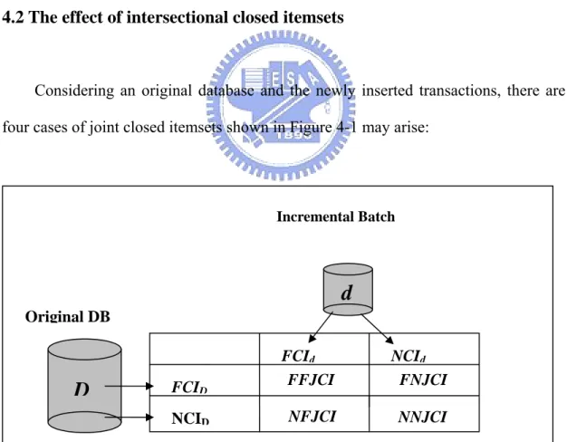
(20) Case 1 of Lemma 2, contradicting the claim that x ∉ CId. Thus y ⊆/ z and z ⊆/ y. According to Case 2 of Lemma 2, there must exist x’ = y ∩ z and x’ ∈ CID+. If x ⊂ x’, x is closed by x’ (because x’.supD+ = x.supD+), contradicting the claim that x ∈ CID+. Thus, x = x’ and x ∈ JCI.. . Theorem 1: CID+ = CID ∪ CId ∪ JCI. Proof: According to Lemmas 1 and 2, we have (CID ∪ CId ∪ JCI) ⊆ CID+. On the other hand, according to Lemma 3, we have CID+ ⊆ (CID ∪ CId ∪ JCI). Thus, CID+ = CID ∪ CId ∪ JCI.. . 4.2 The effect of intersectional closed itemsets. Considering an original database and the newly inserted transactions, there are four cases of joint closed itemsets shown in Figure 4-1 may arise:. Incremental Batch. d Original DB. D. FCID NCID. FCId FFJCI. NCId FNJCI. NFJCI. NNJCI. Figure 4-1: Four cases of JCI. 14.

(21) The case of FFJCI: A closed itemset is frequent in both the original database and the newly inserted transactions. The case of FNJCI: A closed itemset is frequent in the original database but infrequent in the newly inserted transactions. The case of NFJCI: A closed itemset is infrequent in the original database but frequent in the newly inserted transactions. The case of NNJCI: A closed itemset is infrequent in both the original database and the newly inserted transactions.. Since the closed itemsets in FFJCI are frequent in both the original database and the new transactions, they will still be frequent after the weighted average of the counts. Similarly, the closed itemsets in NNJCI will still be infrequent after the new transactions are inserted. FFJCI and NNJCI will not affect the final association rules. FNJCI may remove existing association rules, and NFJCI may add new association rules.. According to Theorem 1, the following theorems are derived to obtain CO and CP by FCID, FCId and JCI.. Theorem 2: CO = {x|x ∈ FCID ∪ FFJCI ∪ FNJCI}. Proof: By definition, CO collects the closed itemsets for D+ which is generated from FID. According to Theorem 1, CO = {x|x ∈ FID and x ∈ CID+} = {x|x ∈ FID and x ∈ CID ∪ CId ∪ JCI } = {x|x ∈ FCID ∪ FFJCI ∪ FNJCI}.. . Theorem 3: CP = {x|x ∈ (FCId − FFJCI) ∪ NFJCI}. Proof: By definition, CP collects the closed itemsets for D+ which is generated 15.

(22) from FId−FID. As Theorem 2, FCId ∪ FFJCI ∪ NFJCI is the set of closed itemsets for D+ which is generated from FId. Thus CP = {x|x ∈ FId − FID and x ∈ CID+} = {(FCId ∪ FFJCI ∪ NFJCI) − (FCID ∪ FFJCI ∪ FNJCI)) = {x|x ∈ FCId ∪ FFJCI ∪ NFJCI – FFJCI} = {x|x ∈ (FCId − FFJCI) ∪ NFJCI}.. . In contrast to the definitions of CO and CP, Theorems 2 and 3 provide a convenient way to obtain CO and CP. For CO, FFJCI and FNJCI can be obtained by processing the pre-stored mining information FCID against d. For CP, however, since NFJCI has to be generated from NCID, which is usually unknown in a typically incremental mining process, this cost is too expensive to be acceptable. As a result, the following theorem is derived to obtain CP.. Theorem 4: CP = {x|x ∈ FId – cover(FFJCI, FId), x ∈ CID+}. Proof: By definition, the FFJCI covers the itemsets which are included both in FId and FID. Thus CP = {x|x ∈ FId − FID and x ∈ CID+} = {x|x ∈ FId – cover(FFJCI, FId), x ∈ CID+}, where the function cover(FFJCI, FId) means the itemsets in FId which are covered by FFJCI.. . Since FFJCI has been obtained in CO generation, we only need to find FId and remove the itemsets in FId which have been determined in FFJCI as candidates for CP. It seems to be a better way for CP generation, because the cost of checking closure property of {FId – cover(FFJCI, FId)} in D+ is less than that of NFJCI generation.. 16.

(23) Chapter 5: The CIM Algorithm According to Theorems 2 and 4, we develop a novel incremental mining algorithm mainly consisting of CO_generation and CP_generation subroutines, called Closed Itemsets Maintaining (CIM), to efficiently find FCID+ for D+. In the proposed CIM algorithm, an in-memory data structure called closed maintenance tree (CMT) is used to facilitate the processes of CO_generation and CP_generation subroutines. The detail of CMT will be illustrated in Section 5.1. When new transactions are inserted, the CIM algorithm first executes the CO_generation subroutine to update existing FCID in CMT and find FFJCI and FNJCI. After that, it executes the CP_generation subroutine to generate the candidate itemsets for CP which has not been determined in the CO_generation subroutine and insert them into CMT. Finally, the CIM algorithm rescans these obtained candidates in CMT against D, checks their closure property and then output the frequent closed itemsets for the updated database. Detail of the proposed CIM algorithm is shown as follows.. The CIM algorithm(CMT, D, d, minsup) Parameters: CMT: A closed maintenance tree; D: An original database; d: A set of newly inserted transactions; minsup: A minimum support. Begin Set FFJCISet = φ;. /* FFJCISet is a set used to store the itemsets of FFJCI. */. Set CandCP1 = φ;. /* CandCP1 is a set used to store candidate 1-itemsets for CP. */ CO_generation subroutine(CMT, d, minsup, FFJCISet, CandCP1); Set F1D+ = φ;. /* F1D+ is a set used to store frequent 1-itemsets in the updated database. */ 17.

(24) Set mincountD+ = minsup * (|D| + |d|); Obtain_frequent_items(CMT, mincountD+, F1D+); /* Obtain F1D+ from CMT. */ CP_generation subroutine(CMT, d, minsup, FFJCISet, CandCP1, F1D+, CMT.root); Rescan_CP(CMT, D, minsup); Check_Closure_CP(CMT); Remove_NI(CMT, mincountD+); Output_FCI(CMT);. /* Rescan obtained candidate k-itemsets (k ≥ 2) of CP in CMT against D. */ /* Check closure property for all candidates itemsets of CP in CMT. */ /* Remove the itemsets in CMT whose support counts are less than mincountD+. */ /* Output the frequent closed itemsets for the updated database.*/. End.. 5.1 The closed maintenance tree (CMT) A closed maintenance tree (CMT) is a tree structure extended from a prefix tree [39]. A prefix tree is constructed as follows. For each itemset x, a corresponding node vx is built in the prefix tree. Node vx maintains its corresponding itemset with support count, denoted as (itemsets, support count). For any pair of nodes vx and vy corresponding to itemsets x and y, there is a directed edge from vx to vy if x is a parent of y. x is said to be a parent of y if y can be obtained by adding a new item to x (x ⊂ y), and inversely, y is said to be a child of x. Therefore, an itemset has only one parent and more than one child in the constructed prefix tree. Note that, the itemsets in a prefix tree are usually maintained in lexicographic order, and for saving the storage space, each node only maintains the suffix of an itemset regarding its parent node. In particular, unlike a general prefix tree maintaining all itemsets in D, a CMT only maintains FCID and some intermediate mining information from D. There are three types of nodes in a CMT:. 18.

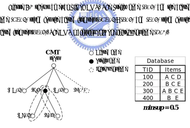
(25) z. Prefix nodes: the nodes are used to represent the common prefixes of closed itemsets.. z. Closed nodes: the nodes are used to represent closed itemsets in FCID. Note that, although a non-leaf closed node also represents the common prefix of its child closed nodes in a CMT, it is not a prefix node mentioned above.. z. Infrequent nodes: the nodes are used to represent infrequent 1-itemsets in D.. The purpose of maintaining infrequent 1-itemsets obtained from D in the CMT is to reduce useless item combinations in the CP_generation subroutine. The detail will be described in Section 5.3.. Figure 5-1 shows an example of CMT. The prefix node (B, 3) and the closed node (CE, 2) stand for the closed itemset (BCE, 2); (B, 3) and (E, 3) stand for the closed itemset (BE, 3). The CMT maintains only one infrequent node (D, 1).. CMT. Closed node. root. Prefix node Infrequent node. (AC, 2). (B,3 ). (C, 3). (D, 1). Database TID 100 200 300 400. Items ACD BCE ABCE B E. minsup = 0.5 (CE, 2). (E, 3). Figure 5-1 A Closed Maintenance Tree. 5.2 Generation of the CO set The CO_generation subroutine is responsible for processing FCID against d to find FFJCI and FNJCI. In that, finding FNJCI is the most concerned because most 19.

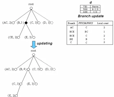
(26) itemsets in NId are needless, thus requiring excessive computation cost. In order to reduce needless item combinations from NId, the CO_generation subroutine adopts the branch-wise processing strategy to find FFJCI and FNJCI. The CO_generation subroutine operates from the most left branch to the most right branch in a given CMT. In each branch, it uses the items belonging to the branch, i.e. the items of the maximum itemset in the branch, as seeds to mine the closed itemsets in d by a closed itemsets mining approach, such as the CHARM algorithm. Since it considers only the items in a branch at a time, needless itemsets belonging to NId can be effectively reduced. After all branches have been processed, the CO_generation subroutine then updates these found itemsets against CMT to obtain CO. Thus, by the branch-wise processing strategy, the CO_generation subroutine can find FFJCI and FNJCI directly and reduce search space of mining closed itemsets in d. The performance of CO_generation subroutine is greatly improved.. Figure 5-2 shows an example of the CO_generation subroutine. Given FCId = {BCD, CD} and NCId = {}. By the branch-wise processing strategy, the CO_generation subroutine first considers the most left branch with items {A, C} and treats {A} and {C} as seeds to mine the closed itemset in d. The item {A} would be removed because it does not appear in d. The found {C} is an itemset belonging to FFJCI. The other branches are processed in a similar way. From this example, the itemset {C} seems to be generated and processed several times and thus increasing computation cost, but in our algorithm, a simple checking mechanism is used to avoid duplicate generation.. 20.

(27) Figure 5-2 an example of branch update strategy. We maintain FCID and infrequent 1-item in the CMT. The CO_generation subroutine updates count of each node in the CMT and inserts new itemsets from FFJCI and FNJCI into the CMT. CO_generation marks all nodes belong to FFJCI that would be used in CP_generation later. It also marks some infrequent 1-item nodes from infrequent to frequent.. CO_generation subroutine(CMT, d, minsup, FFJCISet, CandCP1) Parameters: CMT: The closed maintenance tree; d: The newly inserted transactions; minsup: The minimum support; FFJCISet: The set used to store the itemsets of FFJCI; CandCP1: The set used to store candidate 1-itemsets for CP. Begin Set T = φ;. /* T is a set used to store the mining results by branch-wise processing strategy. */. for each branch bi ∈ CMT, do if bi consists of only one infrequent item x, then 21.

(28) update x.count against d;. /* x.count denotes support count of x. */. if x.count ≥ minsup*|D |, then insert x with x.count into CandCP1; +. else if bi ≠ null, then Closed_itemset_mining(bi, d, T); /* Execute a closed itemsets mining algorithm and store mining results into T. */ x = CMT.get_first_CI(); /* Fetch the first closed itemset by lexical order in CMT. */ y = T.get_first_CI(); /* Fetch the first closed itemset by lexical order in T. */ while x ≠ null and y ≠ null, do if x = y, then x.count = x.count + y.count; if y.count ≥ minsup*|d|, then insert x with x.count into FFJCISet; x = CMT.get_next_CI(x); /* Fetch the next closed itemset by lexical order in CMT. */ y = T.get_next_CI(y); /* Fetch the next closed itemset by lexical order in T. */ else if x ∩ y = x, then x.count = x.count + y.count; if y.count ≥ minsup*|d|, then insert x with x.count into FFJCISet; x = CMT.get_next_CI(x); else if x ∩ y = y then if y.count ≥ minsup*|d|, then insert y with (x.count + y.count) into FFJCISet; y.count = x.count + y.count; insert y with y.count into CMT; y = T.get_next_CI(y); else if x ∩ y = z and z ≠ null then if CMT.exist(z) = false, then z.count = x.count + y.count; insert z with z.count into CMT; if y.count ≥ minsup*|d|, then insert z with z.count into FFJCISet; x = CMT.get_next_CI(x); else if (x.count + y.count) > z.count, then 22.

(29) z.count = x.count + y.count; if y.count ≥ minsup*|d|, then insert z with z.count into FFJCISet; x = CMT.get_next_CI(x); End.. 5.3 Generation of the CP set The CP_generation subroutine is responsible for generating the candidate itemsets for D+ which has not been determined in the CO_generation subroutine. A straightforward way is to find FId and then remove all the itemsets which have been covered by FFJCI. This may require an excessive computation cost for a large size of FId. As a result, the CP_generation subroutine adopts a more effective and efficient way dealing with this task. It attempts to combine the obtained itemsets in FFJCI and the 1-itemsets which are infrequent in D but frequent in D+, denoted as N-F(1), with the frequent 1-itemsets in D+ to directly generate the itemsets belonging to {FId – cover(FFJCI, FId)} as candidates for CP. Since all the infrequent 1-itemsets in D have been pre-retained in the CMT, it is easy to obtain N-F(1) and all the frequent 1-itemsets in D+ after the CO_generation subroutine. Specifically, the CP_generation subroutine first treats each itemset of FFJCI as a seed and each itemset of N-F(1) as an initial candidate. Then it uses a depth-first and left-to-right search manner in the CMT to generate the other candidates. When meeting a seed node vx, an itemset x of FFJCI in the CMT, the CP_generation subroutine combines x with one of the frequent 1-itemsets in D+ to form a new itemset x’. If x’ is not included in one of x’s supersets in FFJCI and frequent in d, x’ is a new candidate itemset and a corresponding node vx’ is built in the CMT. On the other hand, when meeting a candidate node vy, an candidate itemset y of N-F(1) or new itemsets generated above in the CMT, the CP_generation subroutine does a similar combination-and-testing to generate a new 23.

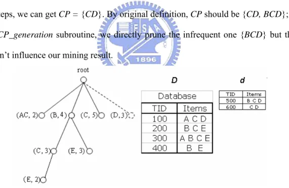
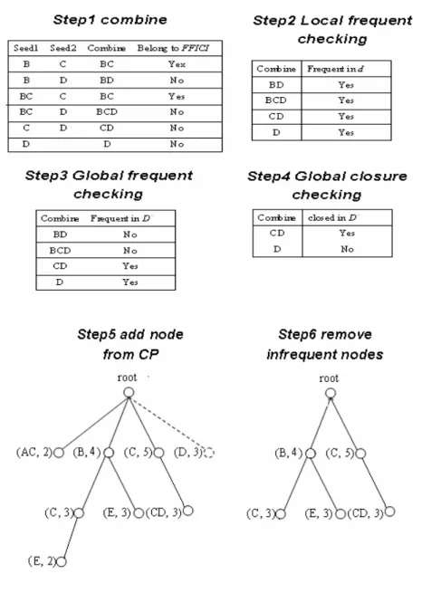
(30) candidate itemset y’ and build a corresponding node vy’ in the CMT. These two candidate generations continue until no new candidate itemsets are generated.. Figure 5-4 extends previous example to show the CP_generation subroutine. The CP_generation subroutine uses FFJCI, {B, BC, C} and newly frequent 1-item {D} to generate CP. At the first step, we fetch the first itemsets {B} and combine all frequent items that are not exist in the supper set of {B} in FFJCI and so on. Since item C appears in itemset {BC}, the superset of {B} in FFJCI. We only have to test {BD} in next step. Second step, we check the combined itemset are local frequent or not. Third step, we rescan D to sure remain itemsets are global frequent or not. At the last step, we will check the support value of remain itemsets and remove the non-closed. After all steps, we can get CP = {CD}. By original definition, CP should be {CD, BCD}; in the CP_generation subroutine, we directly prune the infrequent one {BCD} but this doesn’t influence our mining result.. 24.

(31) Figure 5-3 example of CP_generation CP_generation subroutine(CMT, d, minsup, FFJCISet, CandCP1, F1D+, x) Parameters: CMT: The closed maintenance tree; d: The newly inserted transactions; minsup: The minimum support; FFJCISet: The set used to store the itemsets of FFJCI; CandCP1: The set used to store candidate 1-itemsets for CP; F1D+: The set used to store frequent 1-itemsets in the updated database; x: A variable. Begin if x = CMT.root, then for each child ci of x, do CP_generation subroutine(CMT, d, minsup, FFJCISet, CandCP1, F1D+, ci); 25.

(32) else if x ⊆ FFJCISet or x ⊆ CandCP1, then for each zi ∈ F1D+ and the lexical order of zi is after that of the first item of x, do x’ = combine(x, zi); /* Attempt to generate a new candidate itemset for CP. */ if x’ ≠ null, then if cover(FFJCISet, x’) ≠ null, then continue; /* If x’is covered by FFJCISet. */ update x’.count against d; if x’.count ≥ minsup*|d|, then insert x’ with x’.count into CMT; for each child ci of x, do CP_generation subroutine(CMT, d, minsup, FFJCISet, CandCP1, F1D+, ci); End.. 26.

(33) Chapter 6: The CIM Algorithm with Pre-large Concept: CIM-P Algorithm Although the CIM algorithm focuses on the newly inserted transactions and thus saves much processing time in maintaining association rules, it must still scan D to handle CP in which candidate closed itemsets are frequent for d but not retained in CO. This situation may occur frequently, especially when d is heterogeneous with D. For example, in an extreme case, suppose {A}, {B} and {AB} are the entire CO and {C}, {D} and {CD} are the itemsets in CP. The final results can not be determined without re-processing {C}, {D} and {CD} against D. If the itemsets in CP could be decided without rescanning D at each time, the maintenance time could be further reduced.. 6.1 The concept of pre-large closed itemsets In general, the number of records in d is much smaller than the number of records in D. Only the closed itemsets whose supports are slightly less than minsup in D are possible to be frequent for D+ after database maintenance. The concept of pre-large closed itemsets is denoted as the set of closed itemsets having support between a lower support threshold, which is smaller than minsup, and an upper support threshold, which is equal to minsup. The pre-large closed itemsets are not truly frequent at present but more possible to be frequent in the future when database is updated. Therefore, using the pre-large closed itemsets to enlarge the amount of CO can reduce the cost of rescanning D at the expense of storage spaces. This is because they act as a buffer to avoid the movements of closed itemset directly from infrequent to frequent and vice-versa during the incremental mining process. When few new. 27.

(34) transactions are inserted, the infrequent closed itemsets excluding the pre-large ones will at most become pre-frequent (pre-large) and cannot become frequent. Base on the concept of pre-large closed itemsets, the enhancement of CIM algorithm, CIM-P, does not require rescanning D until the accumulative amount of new transactions exceeds the safety bound the buffer can afford, which depends on database size. Thus, as databases grow larger, the numbers of new transactions allowed before database rescanning is required also grow. The CIM-P algorithm thus becomes increasingly efficient as databases grow.. Figure 6-1 shows the concept of pre-large closed itemsets. The lower support is denoted Sl and the upper support is denoted Su which is equal to minsup. Minsup. Area of small CIs. Area of large CIs support. Area of pre-large CIs. Area of small CIs. Area of large CIs support Sl. Su. Figure 6-1: The concept of pre-large closed itemsets. As mentioned above, if the number of records in d is much smaller than the number of records in D, an itemsets in CP cannot possibly be frequent for D+. Given the user-specified Sl and Su, the safety bound of buffer can be derived by the following theorem. Theorem 5: If |d| ≤. ( Su − Sl ) D 1 − Su. , then an itemsets in CP cannot possibly be. frequent for D+ [22].. . 28.

(35) The. ( Su − Sl ) D 1 − Su. can be used as the safety bound of buffer to decide the suitable. time of rescanning D. However, only considering whether the accumulative amount of new transactions exceeds safety bound. ( Su − Sl ) D 1 − Su. ( Su − Sl ) D 1 − Su. seems too loose. For example, assume the. = 10 and the accumulative amount of new transactions t =. 0. When an increment d, in which each transaction consists of only one distinct item and |d| = 11, has been inserted into D, then t = 11 larger than. ( Su − Sl ) D 1 − Su. = 10 and. the CIM-P algorithm needs rescanning D to cope with CP. However, these distinct closed itemsets consume only one of buffer, and the effort of rescanning D is worthless.. In this study, the bucketing strategy is proposed to improve the utility of buffer. The purpose of bucketing strategy is using some buckets to record the actual contributions of d for the major itemsets, the itemsets with higher support counts, in CP. The consumption of buffer can be tightly calculated using the maximum value of buckets. If only one bucket exists, the bucket is accumulated using the maximum support count in CP. Otherwise, according to the number of buckets k, the bucketing strategy selects k itemsets with the highest support counts in CP and then accumulates their corresponding bucket values: (a) for each selected itemset matching a previously stored itemset in the buckets, the bucketing strategy accumulates the target bucket using the support count of the selected itemset; (b) for the remaining selected itemsets, the bucketing strategy finds two of them respectively having the largest and the smallest support counts to accumulate the unprocessed bucket having the smallest value and all the remaining unprocessed buckets, respectively.. 29.

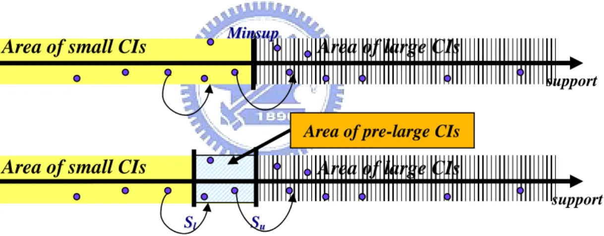
(36) For example, given three buckets b1, b2 and b3, |D| = 100, Sl = 30%, Su = 50%, and CP1 = {(ab, 15), (cd, 12), (cde, 11), (bd, 10)} and CP2 = {(bcd, 11), (ab, 10), (ad, 10)} respectively obtained from two increments with |d1| = 20 and |d2| = 20. By Theorem 5, the safety bound is. (0.5 − 0.3) * 100 = 40 . After d1 has been inserted into 1 − 0.5. D, b1 = (ab, 15), b2 = (cd, 12) and b3 = (cde, 11). Since the maximum value of buckets is 15 less than 40, the CIM-P algorithm does not need rescanning D and the safety bound becomes. (0.5 − 0.3) * 120 + = 48 in the updated database D . After d2 has been 1 − 0.5. inserted into D+, the bucketing strategy first accumulates b1 = (ab, 15) using the support count of (ab, 10) and thus b1 = (ab, 25), and then accumulates b2 = (cd, 12) and b3 = (cde, 11) respectively using the support count of (ad, 10) and (bcd, 11) and thus b2 = (ad, 22) and b3 = (bcd, 22). Since the maximum value of buckets is 25 less than 48, the CIM-P algorithm still does not need rescanning D+.. The utility of buffer would be better if we have more buckets, but the cost of storage space and accumulating buckets would be increased. This is a trade off in this strategy. In the CIM-P algorithm, according to the user-specified lower support and upper support thresholds, the large and pre-large closed itemsets with their support counts in preceding runs are stored in the CMT for later use in maintenance. When new transactions are inserted, the proposed algorithm first executes the CO_generation subroutine to find FFJCI and FNJCI and the CP_generation subroutine to generate the candidate frequent closed itemsets for D+ which has not been determined in the CO_generation subroutine. Then, the proposed algorithm utilizes the bucketing strategy to calculate the accumulative consumption of buffer and decide the suitable time of rescanning D. If the accumulative consumption is 30.

(37) within the safety bound of buffer, no action is needed. Otherwise, the original database has to be re-scanned to guarantee information lossless. The detail of the proposed maintenance algorithm is shown as follows.. 6.2 The detail Algorithm of CIM-P In the CIM-P algorithm, according to the user-specified lower support and upper support thresholds, the large and pre-large closed itemsets with their support counts in preceding runs are stored in the CMT for later use in maintenance. When new transactions are inserted, the proposed algorithm first executes the CO_generation subroutine to find FFJCI and FNJCI and the CP_generation subroutine to generate the candidate frequent closed itemsets for D+ which has not been determined in the CO_generation subroutine. Then, the proposed algorithm utilizes the bucketing strategy to calculate the accumulative consumption of buffer and decide the suitable time of rescanning D. If the accumulative consumption is within the safety bound of buffer, no action is needed. Otherwise, the original database has to be re-scanned to guarantee information lossless. The detail of the proposed maintenance algorithm is shown as follows.. The CIM algorithm(CMT, D, d, Sl, Su, k) Parameters: CMT: A closed maintenance tree based on Sl; D: An original database; d: A set of newly inserted transactions; Sl: A lower support threshold; Su: An upper support threshold; k: the number of buckets. Begin Set SF =. ( Su − Sl ) D 1 − Su. ;. /* SF is the safety bound of buffer*/. 31.

(38) Set FFJCISet = φ;. /* FFJCISet is a set used to store the itemsets of FFJCI. */. Set CandCP1 = φ;. /* CandCP1 is a set used to store candidate 1-itemsets for CP. */. Set_Bucket(BucketSet, 0, φ). /* Initiate buckets, where BucketSet is a set used to store the most frequent k itemsets in CP*/ CO_generation subroutine(CMT, d, Su, FFJCISet, CandCP1); Set F1D+ = φ;. /* F1D+ is a set used to store frequent 1-itemsets in the updated database. */. Set mincountD+ = Su * (|D| + |d|); Obtain_frequent_items(CMT, mincountD+, F1D+); /* Obtain F1D+ from CMT. */ CP_generation subroutine(CMT, d, minsup, FFJCISet, CandCP1, F1D+, CMT.root); if Bucket_Strategy(CMT, BucketSet, Su) > SF, then /* return support count of most frequent itemset in the Bucket */ Rescan(CMT, D, d, Sl); /* Reconstruct CMT based on Sl */ else, Remove_NI(CMT, mincountD+); Output_FCI(CMT);. /* Remove the itemsets in CMT whose support counts are less than mincountD+. */ /* Output the frequent closed itemsets for the updated database.*/. End.. 32.

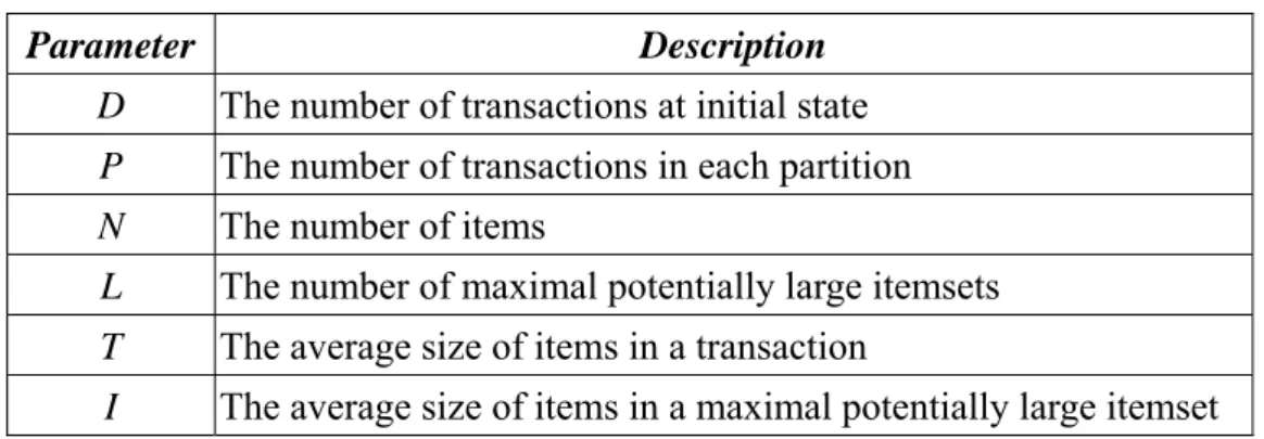
(39) Chapter 7: Experiments Before showing the experimental results, we first describe the experimental environments and the datasets used.. 7.1. The experimental environment and the datasets used. The experiments were implemented in C++ on a workstation with dual XEON 2.8GHz processors and 2048MB main memory, running RedHat 9.0 operating system. Several synthetic datasets and a real-world dataset called BMS-POS [3835] were used in our experiments. The synthetic datasets were generated by a generator similar to that used in [4]. The parameters listed in Table 1 were considered when generating the datasets. The generator first generated L maximal potentially large itemsets, each with an average size of I items. The items in a potentially large itemset were randomly chosen from the total N items according to its actual size. The generator then generated D transactions, each with an average size of T items. The items in a transaction were generated according to the L maximal potentially large itemsets in a probabilistic way. The details of the dataset generation process can be referred to in [4]. Table 1: The parameters considered when generating the datasets Parameter. Description. D. The number of transactions at initial state. P. The number of transactions in each partition. N. The number of items. L. The number of maximal potentially large itemsets. T. The average size of items in a transaction. I. The average size of items in a maximal potentially large itemset. 33.

(40) The two synthetic datasets generated and used in our experiments are listed in Table2. Table2: Two synthetic datasets Datasets T10I8D10K T10I8D500K. D. P. T. I. L. N. 70000. 5000. 10. 8. 200. 145. 2000000 100000 10. 8. 400 to 560. 200. The BMS-POS dataset contains several years of point-of-sale data from a large electronics retailer. Each transaction in this dataset is a customer’s purchase transaction consisting of all the product categories purchased at one time. There are 515,597 transactions in the dataset. The number of distinct items is 1,657, the maximal transaction size is 164, and the average transaction size is 6.5. This dataset was also used in the KDDCUP 2000 competition. In our experiments, D = 500000 and P = 1000 from the BMS-POS dataset.. 7.2. The experimental results. In addition to our proposed CIM and CIM-P algorithm, a closed itemsets mining algorithm, CHARM was then run for two synthetic datasets requests. The CHARM algorithm reprocesses entire dataset when a new partition of data is inserted. The CIM and CIM-P algorithms treated each partition as a new addition of transactions. For the synthetic data, the execution time spent by the three algorithms for the two datasets is shown in Figure7-1.. We first compare the CIM and CIM-P algorithms with the CHARM algorithm. From Figures 7-1(a) and 7-1(c), it is easily seen that the execution times by the CIM. 34.

(41) and CIM-P algorithms for different transactions are very small. The execution times by the CHARM algorithm are much larger than those by the CIM and CIM-P algorithm, and increase proportional to the numbers of transactions. It can thus be concluded that the CIM and CIM-P becomes increasingly efficient as the database grows.. In Figure 7-1(b) and 7-1(d), the execution time was recorded after updating the first new partition in different support values. It is easily seen that these three algorithms have similar tendencies. The decrement of execution time and the increment of support value is an inverse proportion. CIM and CIM-P need more execution time than CHARM because CIM and CIM-P have to record mining lots of information at the first partition.. Dataset T10I8D10K 7-1(a): The relationships between computational times and partition numbers.. 35.

(42) Dataset T10I8D10K 7-1(b): The relationships between computational times and support values.. Dataset T10I8D500K 7-1(c): The relationships between computational times and partition numbers.. Dataset T10I8D500K 7-1(d): The relationships between computational times and support values. Figure7-1: The execution time spent by the three algorithms for two synthetic datasets. Finally, we compare the CIM algorithm with the CIM-P algorithm. In our experiments, CIM-P spent more execution time than CIM in both datasets. The first reason is CIM-P has to record more information than CIM at the first partition thus CIM-P spent more time at the first partition. We believe the CIM-P would outperform CIM if we used more partitions in our experiment. The second reason is the lower support Sl is too low and we will test the influence of Sl in the future. 36.

(43) In the second part of the experiments, the real-world BMS-POS [38] dataset was used. The execution time spent by the three algorithms for this dataset is shown in Figure7-2. The CIM and CIM-P algorithms still outperform CHARM when the number of partitions is increased. But there exists an interesting situation in Figure 7-2(b), both CIM and CIM-P need less execution time than CHARM. It is because in the real dataset, BMS-POS, there are less information be recorded since the less frequent closed itemsets are generated in the first partition... 7-2(a): The relationships between computational times and partition numbers.. 7-2(b): The relationships between computational times and support values. Figure7-2: The execution time spent by the three algorithms on the real-world BMS-POS dataset. 37.

(44) Chapter 8: Conclusion. Designing incremental mining algorithms which effectively utilize the previously mined information to reduce costs of knowledge maintenances is rather important and useful. In order to compress the amount of frequent itemsets, we have utilized the concepts of closed itemsets to develop more efficient, scalable and practical approaches for maintaining and compressing association rule. In the first part of this thesis, we have described that is not an intuitive translation from incremental frequent itemsets mining to incremental frequent closed itemsets mining, and divided the closed itemsets in the updated database into several portions. We have shown the frequent closed itemsets in the updated database could be generated by two candidate sets, the closed original frequent itemsets and the closed potentially frequent itemsets. A special set named intersectional closed itemset collects the closed itemsets that only appears in the updated database has also been described. Some frequent closed itemsets belong to the intersectional closed itemsets are difficult to be determined since they were closed by other closed itemsets before. We have shown the relations between the closed original itemsets, the closed potentially frequent itemsets and intersectional closed itemsets. In the second part of this thesis, in order to avoid huge comparing cost, CIM has utilized the branch update strategy to generate the closed original frequent itemsets and make full use of the closed original itemsets to generate the closed potentially frequent itemsets are generated from . At last we have utilized the concept of pre-large, to develop the CIM-P algorithm that reduces the amount of the closed potentially frequent itemsets further. We have utilized two strategies to improve the utility of. 38.

(45) buffer. The first is bucketing strategy that uses some buckets to record the actual contributions of d for the major itemsets in pre-large (the itemsets with higher supports). The consumption of buffer can be tightly calculated using the maximum value of buckets. This strategy can enhance the utility of buffer and the second strategy is using the infrequent 1-items to prune the itemsets that must still be infrequent. These two strategies can enhance the utility of buffer used in our CIM-P algorithm.. 39.

(46) Reference 1. C.C. Aggarwal, P.S. Yu, A new approach to online generation of association rules, IEEE Transactions on Knowledge and Data Engineering, Vol. 13, No. 4, pp. 527-540, 2001. 2. R. Agrawal, T. Imielinksi, A. Swami, Mining association rules between sets of items in large database, ACM SIGMOD Conference, pp. 207-216, Washington DC, USA, 1993. 3. R. Agrawal, T. Imielinksi, A. Swami, Database mining: a performance perspective, IEEE Transactions on Knowledge and Data Engineering, Vol. 5, No. 6, pp. 914-925, 1993 4. R. Agrawal, R. Srikant, Fast algorithm for mining association rules, ACM International Conference on Very Large Data Bases, pp. 487-499, 1994. 5. R. Agrawal, R. Srikant, Mining sequential patterns, IEEE International Conference on Data Engineering, pp. 3-14, 1995. 6. W.G. Aref, M.G. Elfeky, A.K. Elmagarmid, Incremental, online, and merge mining of partial periodic patterns in time-series databases, IEEE Transactions on Knowledge and Data Engineering, Vol. 16, No. 3, pp. 332-342, 2004. 7. R.J. Bayardo, R. Agrawal, D. Gunopulos, Constraint-based rule mining in large, dense databases, IEEE International Conference on Data Engineering, pp. 188-197, 1999. 8. K. Beyer, R. Ramakrishnan, Bottom-up computation of sparse and iceberg cubes, ACM SIGMOD Conference, pp. 359-370, 1999. 9. S. Brin, R. Motwani, C Silverstein, Beyond market baskets: generalizing association rules to correlations, ACM SIGMOD Conference, pp. 265-276, Tucson, Arizona, USA, 1997. 40.

(47) 10. S. Brin, R. Motwani, J.D. Ullman, S. Tsur, Dynamic itemset counting and implication rules for market basket data, ACM SIGMOD Conference, pp. 255-264, Tucson, Arizona, USA, 1997. 11. S. Chaudhuri, U. Dayal, An overview of data warehousing and OLAP technology, ACM SIGMOD Record, 26:65-74, 1997. 12. M.S. Chen, J. Han, P.S. Yu, Data mining: an overview from database perspective, IEEE Transactions on Knowledge and Data Engineering, Vol. 8, No. 6, pp. 866-883, 1996. 13. D.W. Cheung, J. Han, V.T. Ng, C.Y. Wong, Maintenance of discovered association rules in large databases: an incremental updating approach, IEEE International Conference on Data Engineering, pp. 106-114, 1996. 14. D.W. Cheung, S.D. Lee, B. Kao, A general incremental technique for maintaining discovered association rules, In Proceedings of Database Systems for Advanced Applications, pp. 185-194, Melbourne, Australia, 1997. 15. M. Fang, N. Shivakumar, H. Garcia-Molina, R. Motwani, J.D. Ullman, Computing iceberg queries efficiently, ACM International Conference on Very Large Data Bases, pp. 299-310, 1998. 16. R. Feldman, Y. Aumann, A. Amir, H. Mannila, Efficient algorithms for discovering frequent sets in incremental databases, ACM SIGMOD Workshop on DMKD, pp. 59-66, USA, 1997. 17. G. Grahne, L.V.S. Lakshmanan, X. Wang, M.H. Xie, On dual mining: from patterns to circumstances, and back, IEEE International Conference on Data Engineering, pp. 195-204, 2001. 18. J. Han, L.V.S. Lakshmanan, R. Ng, Constraint-based, multidimensional data mining, IEEE Computer Magazine, pp.2-6, 1999. 19. J. Han, M. Kamber, Data mining: concepts and techniques, Morgan Kaufmann 41.

(48) Publishers, 2001. 20. J. Han, J. Pei, Y. Yin, Mining frequent patterns without candidate generation, ACM SIGMOD Conference, pp. 1-12, 2000. 21. C. Hidber, Online association rule mining, ACM SIGMOD Conference, pp. 145-156, USA, 1999. 22. T.P. Hong, C.Y. Wang, Y.H. Tao, A new incremental data mining algorithm using pre-large itemsets, International Journal on Intelligent Data Analysis, 2001. 23. W.H. Immon, Building the data warehouse, Wiley Computer Publishing, 1996. 24. L.V.S. Lakshmanan, R. Ng, J. Han, A. Pang, Optimization of constrained frequent set queries with 2-variable constraints, ACM SIGMOD Conference, pp. 157-168, Philadelphia, Pennsylvania, USA, 1999. 25. B. Lan, B.C. Ooi, K.L. Tan, Efficient indexing structures for mining frequent patterns, IEEE International Conference on Data Engineering, pp. 453-462, 2002. 26. H. Mannila, H. Toivonen, A.I. Verkamo, Efficient algorithm for discovering association rules, The AAAI Workshop on Knowledge Discovery in Databases, pp. 181-192, 1994. 27. H. Mannila, H. Toivonen, On an algorithm for finding all Interesting sentences, The European Meeting on Cybernetics and Systems Research, Vol. II, 1996. 28. R.T. Ng, L.V.S. Lakshmanan, J. Han, A. Pang, Exploratory mining and pruning optimizations of constrained associations Rules, ACM SIGMOD Conference, pp. 13-24, Seattle, Washington, USA, 1998. 29. J.S. Park, M.S. Chen, P.S. Yu, Using a hash-based method with transaction trimming for mining association rules, IEEE Transactions on Knowledge and Data Engineering, Vol. 9, No. 5, pp. 812-825, 1997. 30. N.L. Sarda, N.V. Srinivas, An adaptive algorithm for incremental mining of association rules, IEEE International Workshop on Database and Expert Systems, 42.

(49) pp. 240-245, 1998. 31. A. Savasere, E. Omiecinski, S. Navathe, An efficient algorithm for mining association rules in large databases, ACM International Conference on Very Large Data Bases, pp. 432-444, 1995. 32. S. Thomas, S. Bodagala, K. Alsabti, S. Ranka, An efficient algorithm for the incremental update of association rules in large databases, The International Conference on Knowledge Discovery and Data Mining, pp. 263-266, 1997. 33. K. Wang, L. Tang, J. Han, J. Liu, Top down FP-Growth for association rule mining, Pacific-Asia Conference on Advances in Knowledge Discovery and Data Mining, pp. 334-340, 2002. 34. N. Pasquier, Y. Bastide, R. Taouil, and L. Lakhal. Discovering frequent closed itemsets for association rules. In ICDT'99, Jan. 1999. 35. J. Pei, J. Han, and R. Mao. CLOSET: An efficient algorithm for mining frequent closed itemsets. In DMKD'00, May 2000. 36. M. Zaki and C. Hsiao. CHARM: An efficient algorithm for closed itemset mining. In SDM'02, April 2002. 37. J. Wang, J. Han, and J. Pei, “Closet+: Searching for the Best Strategies for Mining Frequent Closed Itemsets,” Proc. ACM SIGKDD Int’l Conf. Knowledge Discovery and Data Mining, Aug. 2003. 38. Z. Zheng, R. Kohavi, L. Mason, Real world performance of association rule algorithms, The International Conference on Knowledge Discovery and Data Mining, 2001. 39. R. C. Agarwal, C. C. Aggarwal, and V. V. V. Prasad. A tree projection algorithm for generation of frequent item sets. Journal of Parallel and Distributed Computing, 61(3):350– 371, 2001.. 43.

(50)