國
立
交
通
大
學
資訊工程系
博
士
論
文
由二維影像序列建構三維物體幾何模型
Constructing 3D Object Models from Image
Sequences
研 究 生:周宏隆
指導教授:陳 稔 教授
由二維影像序列建構三維物體幾何模型
Constructing 3D Object Models from Image Sequences
研 究 生:周宏隆 Student:Hong-Long Chou
指導教授:陳 稔 Advisor:Zen Chen
國 立 交 通 大 學
資 訊 工 程 系
博 士 論 文
A DissertationSubmitted to Department of Computer and Information Science College of Electrical Engineering and Computer Science
National Chiao Tung University in partial Fulfillment of the Requirements
for the Degree of Doctor of Philosophy
in
Computer Science and Information Engineering
July 2004
Hsinchu, Taiwan, Republic of China
由二維影像序列建構三維物體幾何模型
研究生:周 宏 隆 指導教授:陳 稔 博士
國立交通大學資訊工程學系
摘要
本論文提出四個利用二維影像序列建構三維物體幾何模型的方法。首先,我 們透過物體輪廓線及相機成像中心的連線,產生不同視角的成像空間。透過成像 空間的交集,我們可以產生物體的八分樹表示式。因為有限的時間及空間資源限 制,傳統上使用者透過指定最大八分樹細分階層來控制八分樹建構程序終止於資 源殆盡之前。此方式之缺點在於使用者無法由所設定之參數推估建構出的模型和 實際物體的差異。再者,八分樹節點無論投影誤差大小,皆須細分到指定的最大 八分樹細分階層。在此論文中,我們提出一個投影誤差上限的概念。在前兩個方 法,透過投影誤差的計算及比較,我們分別定義新的灰色八分樹節點。利用此新 定義的灰色八分樹節點,我們提出兩個投影誤差控制的快速八分樹建構程序。不 只是以實驗證明,在相同的建構模型品質下,我們所提出的方法在空間需求及運 算時間上皆優於傳統的八分樹建構方法,我們亦在理論上得到相同的驗證。 在第三個方法中,我們提出一個最佳八分樹遊走演算法。我們利用八分樹節 點投影誤差做排序,如此在建構八分樹模型時,可以最大誤差之節點為最優先處 理之節點。實驗及理論上均證明所提出之方法在每單位八分樹節點的處理之誤差 改進效能上皆能比傳統利用深度優先或橫向優先有較佳之表現。 在第四個方法中,我們提出一個未校正相機的平面物體模型建構方法。相較 於前三種方法需要獲知相機內外部參數方可建構物體三維模型,在此方法中,我 們提出一個不需事先校正相機參數的物體模型建構方法。並且,針對平面物體的 建構,我們捨棄利用易受影像雜訊干擾之傳統點特徵的程序。我們透過平面轉換矩陣,直接推導相當的投影矩陣。進而推導出物體組成平面的平面方程式。最後 再利用平面轉換矩陣及平面方程式將不同的建構結果統合在同一個座標系統 中。大量的實驗及雜訊影響分析證明我們的方法是有效且強健的。
Constructing 3D Object Models from Image Sequences
Student:Hong-Long Chou Advisor:Dr. Zen Chen
Department of Computer Science and Information Engineering
National Chiao Tung University
ABSTRACT
Constructing 3D object models from image sequences has gained tremendous attraction in computer vision for the past few decades. The constructed object geometric model finds many applications including robotic system, computer aided design, virtual reality, digital entertainment and target recognition. There are many methods for constructing the object geometric model. Two types of approaches will be addressed in this dissertation: shape from silhouettes and shape fitting with planes. The shape-from-silhouette method is one of the popular techniques used to construct the object shape model from a sequence of object silhouette images. The object silhouette provides important clues of the object shape for human visual system. From the object silhouette and its corresponding viewing position, one can generate a viewing volume encapsulating the object in the particular view. By intersecting the viewing volumes obtained from all viewing directions, a volumetric representation for the object can be generated. However, it often requires a huge memory space to store the 3D object volume even using a hierarchical data structure like octree. Besides, a long computer time is taken to intersect all the viewing volumes to generate the final octree. Another type of construction methods is to fit the 3D object surface with planes. The feature correspondence and robust estimation of the 3D shape of the object are two of the main problems in this type of approaches.
In this dissertation, four different methods for constructing the 3D model of a real object from image sequences are proposed. In the first method, a new octree-based
subdivision strategy of two novel types of “grey” octants is proposed to speed up the octant subdivision process under a construction quality control. To further expedite the construction process a fast way for computing the 3D-to-2D projection of octant vertices using the information of vanishing point and cross ratio is proposed. In the second method, the octant whose image touches the silhouette is further classified into three types of grey octants: grey-grey, grey-black and grey-white. Then those octants having little intersection with object silhouettes will not be subdivided. This method has a great improvement on the computer processing time and memory storage space for a given construction quality specification. In the third method, a progressive mode instead of a recursive mode is proposed for the octree construction. The octree generation will be implemented using a best-first tree traversal scheme instead of a conventional depth first or breadth first tree traversal scheme. The precedence of octants for the arrangement of subdivision is ranked according to the XOR error between the projected octant image and the object silhouette. The progressive octree construction method generally gives the better visual quality rate of the object rendering effect, compared to the conventional recursive construction method.
The fourth construction method is to fit the object surface with planes. The 3D object model construction usually requires camera calibration beforehand. However, it is not easy for a user to calibrate the camera in circumstances, in particular, in the case of a hand-held camera. The fourth method for constructing the object from an uncalibrated image sequence is proposed. Instead of using the point based feature to construct the 3D information, the planar homography defined over an object planar surface is used to derive the projective geometric model of the object.
All of the four construction methods are tested on real and synthetic images. The performance of the methods is evaluated in terms of visual projection error, memory space and processing time. Analytical analysis on each method is also given. The four methods offer the user more choice in constructing the object geometric model to meet the different application requirements.
ACKNOWLEDGEMENTS
I wish to express my sincere appreciation to my advisor, Dr. Zen Chen, for his kind patience, constant encouragement, helpful guidance and inspriation throughout the course of this dissertaion. In these years, he has stimulated the research work and also provided an excellent research environment at the Pattern Analysis and Intelligent System (PAIS) Laboratory. He also teaches me how to learn and how to think indenpdently. Especially, he encourages me to challenge what we are used to be. I also express my sincere gratitude to the members of my thesis committee, Professor Lee and Professor Chuang, for their valuable suggestions and comments.
I am grateful to my fellow classmates in the PAIS Laboratory for their assistannce and discussion, expecially Mr. Y. H. Fang. Special thanks are also due to the alumni of PAIS Lab. It is a pleasure to be with you guys staying up for writing codes and playing baseball or basketball.
A special thank is given to my sister, brother-in-law and brothers for their constant encouragemetn. Finally, I would like to dedicate this dissertation to my parents. Mr. S. S. Chou and Mrs. M. Hsiao for their love, encouragement and support.
TABLE OF CONTENTS
ABSTRACT (in Chinese)………... vii
ABSTRACT (in English)……… ix
ACKNOWLEDGEMENT……..……… xi
TABLE OF CONTENTS……… xii
LIST OF FIGURES……….……… xiv
LIST OF TABLES………..……… xvii
CHAPTER 1 INTRODUCTION ...1
1.1 Statement of the Problem...1
1.2 Survey of Related Research ...1
1.3 Sketch of the Work ...4
1.4 Contribution of the Work...5
1.5 Dissertation Organization ...6
CHAPTER 2 FAST OCTREE CONSTRUCTION ENDOWED WITH AN ERROR BOUND CONTROLLED SUBDIVISION SCHEME ...7
2.1 Introduction...7
2.2 Fast Octant Projection Computation Using Cross Ratio and Vanishing Point 8 2.3 2D Intersection Test Using the Precomputed Distance Maps of Silhouette Images and Approximation of an Octant Image by a Circle ...12
2.4 New Subdivision Strategy and Construction Quality Measure ...14
2.5 Experimental Results ...15
2.6 Analysis on the New Octree Construction Method ...33
2.7 Conclusions and Future Work ...38
CHAPTER 3 AN OCTREE CONSTRUCTION METHOD WITH THREE TYPES OF GREY OCTANTS ...39
3.1 Introduction...39
3.2 Types of New Grey Octants...39
3.3 The Octant Subdivision Algorithm of the Second Construction Method...40
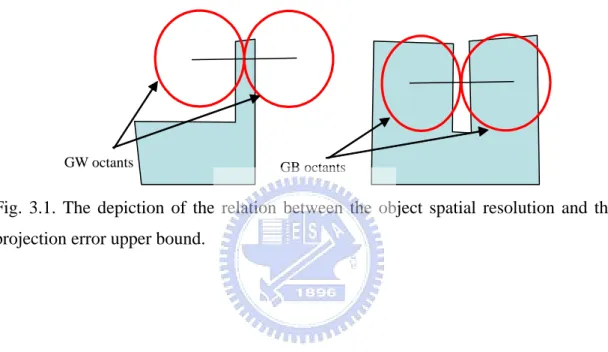
3.4 The Relation between Object Spatial Resolution and Projection Error Upper Bound ...40
3.5 Experimental Results ...41
3.6 Analytical Analysis ...53
3.7 Conclusion ...60
CHAPTER 4 A PROGRESSIVE OCTREE CONSTRUCTION METHOD WITH A PROJECTION ERROR MEASURE ...61
4.2 Depth-First Tree Traversal Scheme vs. Breadth-First Tree Traversal Scheme
...62
4.3 Best-First Tree Traversal Scheme with Octant Sorting Based on Projection Error ...64
4.4 Experimental Results ...67
4.5 Analytical Analysis on the Performance of the Proposed Method ...73
4.6 Conclusion ...79
CHAPTER 5 A NOVEL 3D PLANAR OBJECT RECONSTRUCTION FROM MULTIPLE UNCALIBRATED IMAGES USING THE PLANE-INDUCED HOMOGRAPHIES...80
5.1 Introduction...80
5.2 Preliminaries and Mathematical Notations for Projective Reconstruction....82
5.3 Reconstruction of All Visible Planes from a Given Image Pair ...85
5.4 Integration of Planes Reconstructed from Different Image Pairs ...87
5.5 Computation of Homographies...89
5.6 Experimental Results ...90
5.7 Conclusions...97
CHAPTER 6 SUMMARY AND FUTURE RESEARCH...98
6.1 Summary and Conclusions ...98
6.2 Topics for Future Research...99
REFERENCES ...101
VITA ...106
LIST OF FIGURES
Fig. 2.1. The 27 distinct vertices involved in the subdivision of a parent octant including eight A-type vertices (A0, A1, .., A7), twelve B-type vertices (B0, B1,.., B11), six C-type vertices (C0, C1,..,C5), and one D-type vertex D0. ...9 Fig. 2.2. The four collinear points, p1, p2, p3 andp , together with their 3D∞
corresponding vertices P1, P2, P3 andP , define a common cross ratio value...10 ∞ Fig. 2.3. The illustration of octant subdivision strategy based on the spatial relation
between the circle containing the projected octant and the object silhouette. ...14 Fig. 2.4. The hardware setup of the system. ...15 Fig. 2.5. The schematic diagram of the right cube. The dimensions of the cube are 20
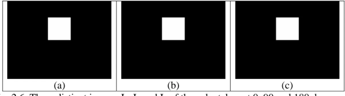
inches in depth (the x-direction), 20 inches in width (the z direction) and 20 inches in height (the y direction). ...16 Fig. 2.6. Three distinct images I0, I3 and I7 of the cube taken at 0, 90 and 180 degrees.
...16 Fig. 2.7. The comparison between construction results of the synthetic cube obtained
by the conventional method and the new method...18 Fig. 2.8. The schematic diagram of the tilted cube. The dimensions of the cube are 20
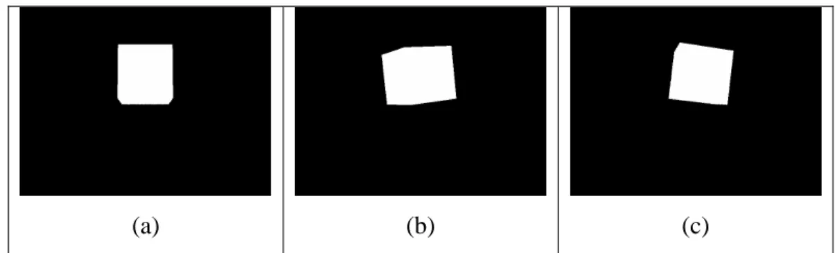
inches in depth (the x-direction), 20 inches in width (the z direction) and 20 inches in height (the y direction). ...19 Fig. 2.9. Three distinct images I0, I3 and I7 of the tilted cube taken at 0, 120 and 280
degrees. ...19 Fig. 2.10. The comparison between the construction results of the synthetic cube
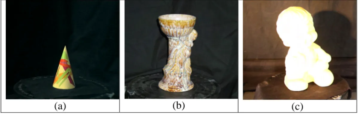
obtained by the conventional method and the new method. ...21 Fig. 2.11. Three real objects used in the experiments: (a) a cone, (b) a vase, and (c) a
boy sculpture. ...21 Fig. 2.12. New views generated from the constructed octree models for (a) a cone, (b)
a vase, and (c) a boy sculpture. The octree models are converted to VRML format and rendered using Cosmo© player. ...22 Fig. 2.13. The comparison between construction results of the cone obtained by the
conventional method and the new method...26 Fig. 2.14. The comparison between construction results of the vase obtained by the
conventional method and the new method...27 Fig. 2.15. The comparison between construction results of the boy sculpture obtained
by the conventional method and the new method...28 Fig. 2.16. The total leaf node number vs. XOR error plot of the construction results
Fig. 2.17. The computation time vs. XOR error plot of the construction results
obtained by the new method and the conventional method. ...32 Fig. 3.1. The depiction of the relation between the object spatial resolution and the
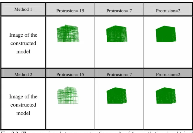
projection error upper bound. ...41 Fig. 3.2. The comparison between construction results of the synthetic cube obtained
by method 1 and method 2...43 Fig. 3.3. The comparison between construction results of the cone obtained by the
conventional method and the new method...49 Fig. 3.4. The comparison between construction results of the vase obtained by the
conventional method and the new method...50 Fig. 3.5. The comparison between construction results of the boy sculpture obtained
by the conventional method and the new method...51 Fig. 3.6. (a) One of the input image to the second method. (b) The new view
generated from the constructed octree model. ...52 Fig. 3.7. (a) One of the input image to the second method. (b) The new view
generated from the constructed octree model. ...52 Fig. 3.8. The depiction of centroids of the bounding circles for an octant and its parent octant and child octant. (Assume rL < p < rL-1 = 2rL)...56 Fig. 3.9. The spatial relation depiction of bounding circles for an octant and its two
sub-octants ...58 Fig. 4.1. A typical octree structure...63 Fig. 4.2. The visiting ordering of the black nodes by the depth-first tree traversal
scheme for the octree in Fig. 4.1...63 Fig. 4.3. The visiting ordering of the black nodes by the breadth-first tree traversal
scheme for the octree in Fig. 4.1...64 Fig. 4.4. The modified insertion process which avoids inserting GB1 octant into the
priority queue. ...65 Fig. 4.5. The modified insertion process which avoids inserting GB2 or GW2 octant
into the priority queue. ...65 Fig. 4-6. The algorithm of the proposed progressive octree construction method. ...66 Fig. 4.7. The constructed octree model of the first 11 octants processed by the DFS
method when viewed from the 1st viewing direction...68 Fig. 4.8. The constructed octree model of the first 11 octants processed by the BFS
method when viewed from the 1st viewing direction...68 Fig. 4.9. The constructed octree model of the first 11 octants processed by the BestFS
method when viewed from the 1st viewing direction...68 Fig. 4.10. The plot of XOR vs. subdivided octant number of the octree model for the
Fig. 4.11. The plot of XOR vs. Subdivided octant number of the octree model for the boy sculpture constructed from the DFS, BFS and BestFS methods. ...70 Fig. 4.12. The priority queue length when constructing the model of the vase using the BestFS_m1 method. ...71 Fig. 4.13. The priority queue length when constructing the model of the vase using the BestFS_m2 method. ...72 Fig. 4.14. The priority queue length when constructing the model of the boy sculpture
using the BestFS_m1 method. ...72 Fig. 4.15. The priority queue length when constructing the model of the boy sculpture
using the BestFS_m2 method. ...73 Fig. 4.16. The relation of radii of the bounding circles for octant Oi and Oj and their
ax_proj_error
( )
Oim and max_ proj_error
( )
Oj . ...75 Fig. 5.1. The flow diagram of our reconstruction method. ...82 Fig. 5.2. The schematic diagram of the tower. The dimensions of the tower are 40inches in depth (the x-direction), 40 inches in width (the z direction) and 180 inches in height (the y direction). ...91 Fig. 5.3. Three distinct images I1, I2 and I3 taken at a distance of about 500 inches.
The visible planes in the three images are ΠGr, ΠA, ΠB, ΠE, ΠF in I1 and I2, and ΠGr, ΠB, ΠF, ΠC, ΠG in I3. ...91 Fig. 5.4. The effects of the uniformly generated reference plane coefficient vectors
and the noise at different levels on the reconstruction result...93 Fig. 5.5. The indices of the vertices and planes of the object. ...95 Fig. 5.6. New views of the reconstructed object with texture mapping...96
LIST OF TABLES
Table 2.1. The comparison of projection computation of octant vertices between the new method and the conventional method...12 Table 2.2 Intersection relation between the projected octant image and a silhouette
image...13 Table 2.3. Numbers of black, grey-black, grey-grey, and white nodes of the cube
generated by our octree construction method with a specified projection error bound...17 Table 2.4. Numbers of black, grey, and white nodes of the cube generated by the
conventional octree construction method with a fixed subdivision level. ...17 Table 2.5. Numbers of black, grey-black, grey-grey, and white nodes of the cube
generated by our octree construction method with a specified projection error bound...18 Table 2.6. Numbers of black, grey, and white nodes of the cube generated by the
conventional octree construction method with a fixed subdivision level. ...20 Table 2.7. Numbers of black, grey-black, grey-grey, and white nodes of the cube
generated by our octree construction method with a specified projection error bound...20 Table 2.8. Numbers of black, grey, and white nodes of the cone generated by the
conventional octree construction method with a fixed subdivision level. ...22 Table 2.9. Numbers of black, grey-black, grey-grey, and white nodes of the cone
generated by our octree construction method with a specified projection error bound...23 Table 2.10. Numbers of black, grey, and white nodes of the vase generated by the
conventional octree construction method with a fixed subdivision level. ...23 Table 2.11. Numbers of black, grey-black, grey-grey, and white nodes of the vase
generated by our octree construction method with a specified projection error bound...24 Table 2.12. Numbers of black, grey, and white nodes of the boy sculpture generated
by the conventional octree method with a fixed subdivision level. ...24 Table 2.13. Numbers of black, grey-black, grey-grey, and white nodes of the boy
sculpture generated by our octree construction method with a specified
projection error bound...25 Table 3.1. Number of the black, grey-black, grey-grey, grey-white and white octants
of the constructed cube generated by method 2...42 Table 3.2. Number of black, grey-black, grey-grey and white octants of the cube
Table. 3.3. The radius range of the circle containing the octant projection at different level...44 Table 3.4. Number of the black, grey-black, grey-grey, grey-white and white octants
of the constructed cone generated by the second construction method. ...44 Table 3.5. Number of black, grey-black, grey-grey and white octants of the cone
generated by the first construction method. ...45 Table 3.6. Number of grey-black and grey-white leaf octants of the cone generated by
applying the second method octant type evaluation criteria on grey-black octants in Table 3.3. ...45 Table 3.7. Number of the black, grey-black, grey-grey, grey-white and white octants
of the constructed vase generated by the second construction method. ...46 Table 3.8. Number of black, grey-black, grey-grey and white octants of the vase
generated by the first construction method. ...46 Table 3.9. Number of grey-black and grey-white leaf octants of the vase generated by
applying the second method octant type evaluation criteria on grey-black octants in Table 3.6. ...47 Table 3.10. Number of the black, grey-black, grey-grey, grey-white and white octants
of the constructed boy sculpture generated by the second construction method. 47 Table 3.11. Number of black, grey-black, grey-grey and white octants of the boy
sculpture generated by the first construction method. ...48 Table 3.12. Number of grey-black and grey-white leaf octants of the boy sculpture
generated by applying the second method octant type evaluation criteria on grey-black octants in Table 3.9. ...48 Table 5.1. 3D object centered coordinates of the tower feature points...92 Table 5.2. The statistics of the distance errors of the reconstruction results. ...92 Table 5.3. The mean errors of the reconstructed Euclidean point positions for different setups...94 Table 5.4. The estimated angles between the object planes and the ground plane...96
CHAPTER 1
INTRODUCTION
1.1 Statement of the Problem
The inference of 3D object geometric model from multiple object images is a key problem in computer vision which finds many applications including robotic system, computer aided design, virtual reality, digital entertainment and target recognition. There are a variety of methods in the literature to construct such a 3D object model. They are characterized by different features such as:
(1) image data acquisition mode: active, passive, …
(2) image processing unit: point, edge, region, contour, texture, shading… (3) object geometric model: voxel-based, surface-based, point-based, …
(4) number of images needed for construction: stereo pairs, triplets, multiple, … (5) camera parameter setting: calibrated, uncalibrated, …
The methods of concern in this dissertation fall under the category characterized by (1) passive sensing,
(2) contour- or region-based,
(3) voxel- or surface-based object model, (4) multiple images required, and
(5) camera-calibrated or -uncalibrated.
The existing methods will be reviewed first in order to point out the drawbacks of these methods. Then new methods will be described which overcome most of the drawbacks discussed, if not all of the drawbacks are removed. Theoretical analysis on the methods will be provided.
1.2 Survey of Related Research
Many 3D structure construction methods have been proposed. They can be classified into:
(B) Passive Vision
The techniques proposed in the active vision class project light pattern onto the object. Then the 3D triangulation or time of light is calculated to estimate the depth information [1]-[10]. Active vision 3D construction methods provide high accuracy results. However, additional procedures are required to set up and calibrate the pattern projection device. Besides, the range of working area is limited to the brightness of the projected light pattern onto the object or scene.
On the contrary, passive vision techniques do not require to project light pattern on the surface to infer the 3D information. Features from the images of the object surfaces are extracted and then used to infer the 3D information. The object silhouette provides an important visual clue which is used to construct the 3D structure of the object. Besides, in the physical world (especially the man-made world) planar surfaces such as walls, windows, table, roof, road, and terrace can be found in the indoor as well as the outdoor scenes. Another task is to reconstruct the 3D planar surfaces in a scene from multiple uncalibrated images taken by a camera placed at different viewpoints. In the following paragraphs, existing methods using the silhouette or planar surfaces information for inferring 3D information are reviewed.
The reconstruction methods using the silhouette information, usually named the silhouette from silhouette (SFS) method, can be further divided into two groups. The first group of methods [11]-[12] applies the differential geometry constraints onto the extracted object silhouettes and generates 3D curves corresponding to the object silhouettes. However, at least three consecutive silhouette images are required to construct the 3D curves. Besides, the change of the object silhouettes should be slightly different, thus a large number of views are required to construct a complete object. Another group of the SFS methods obtain the 3D geometry of the object using the volume intersection techniques. Different structures [13]-[30] have been proposed to represent the initial volume used to intersect with the space that the object occupies. Recently an efficient image-based approach was proposed [66] to compute the so called visual hull of an object to represent the volume where the object occupies. The operation of the method was based on the intersection of the epipolar lines with the silhouette images one by one. The performance of the method is highly dependent on the resolution of the image. Besides, additional rendering techniques, like pixel splating, are required for rendering the new images. In [27][65] methods are proposed to represent the NxNxN voxels to represent the initial volume. They then projected
each voxel onto the images and applied the color consistency check to determine whether the voxel belongs to the object surface or not. The number of N will affect the accuracy of the final result of the constructed model. The larger the N, the better the reconstructed model. However, it will take much time to do the voxel projection and color consistency check. An octree is one of the volumetric representations of an object geometric model. It is well known in the field of computer vision that an octree can be constructed from multiple silhouettes taken from different viewpoints of an object [13]-[24]. They can be divided into two classes: 3D space approach [13]-[16] and 2D space approach [17]-[24]. Both approaches recursively subdivide a partially occupied octree octant into smaller octants until all the generated octants are entirely inside or outside the object. The overlapping between an octree octant and the object is determined by an intersection test. The above two approaches differ in their intersection tests. In the 3D space approach the octant under examination is tested against the conic view volume formed by the individual silhouette and the center of projection for each viewpoint. In the 2D space approach the projection image of the octant is tested against the silhouette for each viewpoint. Generally speaking, the 2D space approach is performed in a space with a lower dimension, so it is more efficient than the 3D space approach [17]. Since the octant number grows exponentially with the subdivision level, an upper bound is usually imposed on the number of subdivision levels to avoid the insufficient memory space problem. However, a larger value of subdivision levels leads to a better construction result. It is generally difficult to make a good balance between memory space and construction quality. In this dissertation, we propose a new subdivision strategy which is governed by the degree of overlapping between the generated octant and the object. We shall consider making effective use of the octant subdivisions to improve the overall system performance.
Recently, much research efforts are involved in developing the 3D geometry reconstruction of an object without calibrating the camera a priori. In general, the methods for 3D projective or uncalibrated reconstruction [33][36][37][40][41][50] are point-based. They estimate the fundamental matrix from a sufficient number of corresponding point pairs first, and then derive the epipole and the canonical geometric representation for projective views using the fundamental matrix. Then, for each pair of corresponding points, they use a triangulation technique or bundle adjustment technique to compute the 3D point coordinates in the projective space. Finally, for the determination of the uncalibrated planar scene structure
[34][39][46][47][49][54][56][60], the 3D points found are fitted by planes. However, it is desirable to derive the 3D planar scene structure in terms of plane features in the images directly, for these features are more reliable than the point or line features [49]. The estimation of the 3D projective planar structure based on the projected plane feature information exclusively has not yet received much attention, although it is known that the corresponding projected plane regions in a pair of stereo images induce a homography. It is also known that homographies are useful to many other practical applications including:
(a) Fundamental matrix estimation or canonical projective geometry representation [48][49].
(b) 2D image mosaicing or view synthesis [43]. (c) Plane + parallax analysis [34][36][56].
(d) Planar motion estimation and ego-motion [45][54][60].
Recently, two methods have been proposed for the 3D projective reconstruction of planes and cameras. The first method assumes all planes are visible in all images and the second method assumes a reference plane is visible in all images [51][52]. In practice, it is not realistic to have all planes or even one plane visible in all images unless a very large ground plane is available. When there is no reference plane visible in all images, the reconstruction problem cannot be formulated within a common projective space and the reconstruction results will be inevitably obtained in different projective spaces.
1.3 Sketch of the Work
In this dissertation, four different methods for constructing the 3D model of a real object from image sequences are proposed. In the first method, a close look at the octant subdivisions reveals that the subdivided octants have varying projection errors; some may be very large and some may be rather small. We shall consider making effective use of the octant subdivisions to improve the overall system performance. In this method, we propose a new subdivision strategy which is governed by the degree of overlapping between the generated octant and the object. This degree of overlapping will be measured by the maximum 2D projection error of the projected octant image relative to the object silhouette for all viewpoints. Those octants with a projection error exceeding the pre-specified upper bound will be subdivided
recursively until all the octants satisfy the maximum constraint imposed on the projection error. Furthermore, we will also present a fast computation of the 2D projection and a new intersection test to reduce the computer processing time.
An extension to the first method is proposed next in the second method. In this method the octant whose image touches the silhouette is further classified into three types of grey octants: grey-grey, grey-black and grey-white. Then those octants having little intersection with object silhouettes will not subdivided. This method has a great improvement on the computer processing time and memory storage space.
A progressive mode instead of a recursive mode is proposed in the third method for the octree construction. The octree generation will be implemented using a best-first tree traversal scheme instead of a conventional depth first or breadth first tree traversal scheme. The precedence of octants for subdivision is ranked according to the XOR error between the projected octant image and the object silhouette. The progressive octree model generally gives the best visual quality rate of the object rendering effect.
The fourth construction method is to fit the object surface with planes. The 3D object model construction usually requires camera calibration beforehand. However, it is not easy for a user to calibrate the camera in circumstances, in particular, in the case of a hand-held camera. The fourth method for constructing the object method from an uncalibrated image sequence is proposed. Instead of using the point based feature to construct the 3D information, the planar homography defined over an object planar surface is used to derive the projective geometric model of the object.
1.4 Contribution of the Work
The contributions of the three proposed octree construction methods are:
(1) The first construction method categorizes the conventional grey nodes into two types and controls the node or octant subdivision by measuring an exclusive OR projection error. Therefore, the ultimate octree subdivision level of the first construction method is not fixed as in the conventional method.
(2) The first construction method outperforms the conventional method in terms of memory space and computation time, given that they have compatible projection errors.
given.
(4) A further improvement over the first construction method is achieved in the second construction method by categorizing the conventional grey nodes into more types of grey nodes.
(5) A progressive, instead of a recursive, reconstruction method achieves with a fast error rate reduction is made possible with a subdivision scheme using the octant sorting based on the projection error.
The contributions of the proposed planar object reconstruction method from uncalibrated images are:
(1) A novel planar object reconstruction method from uncalibrated images is proposed
(2) The estimation of 3D equations of the object planes is directly derived with respect to the assigned reference plane equations and plane-induced homographies.
(3) The integration of the reconstruction results from different images pairs is introduced using the plane-induced homography information.
(4) A performance comparison between our method and the point-based method employing the fundamental matrix with the aid of hallucinated points is provided.
1.5 Dissertation Organization
This dissertation is organized as follows: In Chapter 2, we propose a fast octree construction method with quality control for multiple object silhouette images. Chapter 3 presents the second octree construction method which allows stopping of an octant subdivision if the octant is classified as a “grey-black” octant. In Chapter 4, we propose the third octree construction method which is a progressive method using a priority queue for sorting octants based on the projection errors. In Chapter 5, we propose a novel 3D planar object reconstruction method from multiple uncalibrated images using the plane-induced homographies Chapter 6 is the summary and future work.
CHAPTER 2
FAST OCTREE CONSTRUCTION ENDOWED WITH AN ERROR
BOUND CONTROLLED SUBDIVISION SCHEME
2.1 Introduction
An octree is a volumetric representation of an object geometric model. It is well known in the field of computer vision that an octree can be constructed from multiple silhouettes taken from different viewpoints of an object [1]-[18]. The constructed object geometric model finds many applications including robotic system, computer aided design, virtual reality, and object tracking. The conventional construction methods can be categorized into two classes: 3D space approach [3]-[6] and 2D space approach [7]-[18]. Both approaches recursively subdivide a partially occupied octree octant into smaller octants until all the generated octants are entirely inside or outside the object. The overlapping between an octree octant and the object is determined by an intersection test. The above two approaches differ in their intersection tests. In the 3D space approach the octant under examination is tested against the conic view volume formed by the individual silhouette and the center of projection for each viewpoint. In the 2D space approach the projection image of the octant is tested against the silhouette for each viewpoint. Generally speaking, the 2D space approach is performed in a space with a lower dimension, so it is more efficient than the 3D space approach [7]. Since the octant number grows exponentially with the subdivision level, an upper bound is usually imposed on the number of subdivision levels to avoid the insufficient memory space problem. However, a larger value of subdivision levels leads to a better construction result. It is generally difficult to make a good balance between memory space and construction quality.
A close look at the octant subdivisions reveals that the subdivided octants have varying projection errors; some may be very large and some may be rather small. We shall consider making effective use of the octant subdivisions to improve the overall system performance. In this chapter, we propose a new subdivision strategy which is governed by the degree of overlapping between the generated octant and the object. This degree of overlapping will be measured by the maximum 2D projection error of
the projected octant image relative to the object silhouette for all viewpoints. Those octants with a projection error exceeding the pre-specified upper bound will be subdivided recursively until all the octants satisfy the maximum constraint imposed on the projection error. Furthermore, we will also present a fast computation of the 2D projection and a new intersection test to reduce the computer processing time. A summary of contributions of the chapter is given below:
(1) The ultimate octree subdivision level of the new construction method is not fixed. Instead, it is controlled by a projection error bound.
(2) The construction quality can be evaluated via an exclusive OR projection error. (3) Fast computation of 2D octant projections to the image planes is provided.
(4) Fast 2D intersection test utilizes the distance maps generated for the multiple silhouettes in advance.
(5) Analysis on the properties of the proposed method reveals its superiority over the conventional method in terms of memory space and computation time.
The chapter is organized as follows. Section 2 presents a fast 2D octant projection computation. Section 3 describes the use of distance maps generated from the multiple silhouettes and the approximation of an octant projection image by a circle. Section 4 describes the new subdivision process and the evaluation of the quality of the final octree constructed for the object. Section 5 is the experimental results. Section 6 is the analysis on the new method. Section 7 is the conclusion remarks.
2.2 Fast Octant Projection Computation Using Cross Ratio and Vanishing Point
2.2.1 Computation of perspective projections of octant vertices
When a parent octant is subdivided into 8 child octants, the projection images of these 8 child octants involves 8 x 8 = 64 vertices in the recursive construction process. However, each child octant shares some of its 8 vertices with its siblings. There are 27 (instead of 64) distinct vertices, as shown in Fig. 2.1. We shall compute the perspective projections of the 27 distinct vertices onto the image plane before dividing them into 8 octant projection images.
A0 A1 A3 A2 A7 A6 A5 A4 B0 B3 B2 B1 B5 B4 B6 B7 B11 B10 B8 B9 C0 C1 C3 C2 C4 C5 D0
Fig. 2.1. The 27 distinct vertices involved in the subdivision of a parent octant including eight A-type vertices (A0, A1, .., A7), twelve B-type vertices (B0, B1,.., B11), six C-type vertices (C0, C1,..,C5), and one D-type vertex D0.
There are four types of sub-octant vertices in regard to their parent octant vertices: (i) The A-type vertices in {A0, A1,.., A7}are the vertices belonging to the parent octant. Their perspective projections on the image plane are passed down to the next round of octant subdivision.
(ii) The B-type vertices in {B0, B1,.., B11}are the vertices located on the separate lines defined by pairs of A-type vertices. Their perspective projections on the image plane can be calculated more rapidly from A-type vertices through the use of the cross ratio and vanishing points, as described later.
(iii) The C-type vertices in {C0, C1,..,C5}are the vertices falling on the separate lines defined by pairs of B-type vertices. Their perspective projections on the image plane can be calculated more rapidly from B-type vertices through the use of the cross ratio and vanishing points, too.
(iv) The D-type vertex D0 falls on the line defined by two C-type vertices. Its perspective projections on the image plane can be calculated from C-type vertices through the use of the cross ratio and vanishing point.
In the following the concepts of cross ratio and vanishing point are used to derive the 2D projections of the octant vertices on the image plane.
p∞
p1
p3 p2
Fig. 2.2. The four collinear points, p1, p2, p3 and , together with their 3D corresponding vertices P
∞ p
1, P2, P3 andP∞, define a common cross ratio value.
We only consider the 2D perspective projection computation for a B-type vertex. The other types of octant vertex can be computed similarly. Let a B-type vertex be denoted by P2 and its projected point by p2 and assume it lies on the line between two A-type vertices P1 and P3 whose projected points are p1 and p3, respectively. Let the
point at the infinity along the direction from P1 to P3 be whose vanishing point is
denoted by
∞
P
∞
p
. Figure 2.2 is the depiction of 2D projections of P1, P2, P3 and on the image plane. Then the four collinear points, p∞
P
1, p2, p3 and , together with their
3D corresponding vertices P
∞
p
1, P2, P3 and , define a common cross ratio value [19],
which is invariant under the perspective projection. ∞
P
) p , p , p , (p cr ) P , P , P , (P cr 1 2 3 ∞ = 1 2 3 ∞ , or ∞ ∞ ∞ ∞ ⋅ ⋅ = ⋅ ⋅ p p p p p p p p P P P P P P P P 2 3 1 3 2 1 2 3 1 3 2 1 (2-1) Since P3P∞is equal toP2P∞, ∞ ∞ ⋅ + ⋅ − ⋅ ⋅ = p p p p p p p p p p p p p p p p P P P P 3 3 1 2 1 3 1 3 1 3 1 3 2 1 3 1 2 1 Let 3 1 2 1 P P P P r= (=1/2, as explained below) ∞ ∞ ⋅ + ⋅ − ⋅ ⋅ = p p p p p p p p p p p p p p p p r 3 3 1 2 1 3 1 3 1 3 1 3 2 1 ) p p p p r ( p p p p r p p 3 3 1 1 3 1 2 1 ∞ ∞ + ⋅ = (2-2)A parametric form of the projected line containing the four collinear points, p1, p2, p3 and
p
∞ is given by , ) p (p t p p2 = 1+ ⋅ 3− 1 p∞ = p1+k⋅(p3−p1) with 3 1 1 p p p p k = ∞ and 3 1 2 1 p p p p t= (2-3).Substituting these Equations into Eq. (2-2), we obtain
) 1 k r ( k r t − + ⋅ = .
Since the side length of the child octant equals one half of the side length of the parent octant, r = 1/2. It follows that
) 1 k * 2 ( k t − = (2-4)
The locations of the following three projected points can be read from the image:
T T T v u v u v u , ) ,p ( , ) ,p ( , ) (
p1 = 1 1 3 = 3 3 ∞ = ∞ ∞ . Also the values of k and t can be found
from Eqs. (2-3) and (2-4). Then the projection of the B-type vertex can
be computed from the projections of the two A-type vertices:
T v u , ) ( p2 = 2 2 ) p (p t p p2 = 1+ ⋅ 3− 1 (2-5)
2.2.2 Time Complexity Analysis
Before the analysis of the time complexity of the computation of the projections of octant vertices, recall that in the conventional octree construction method the projection of a 3D octant vertex onto the 2D image is done via a projection matrix H3x4: ⎥ ⎥ ⎥ ⎥ ⎦ ⎤ ⎢ ⎢ ⎢ ⎢ ⎣ ⎡ ⋅ ⎥ ⎥ ⎥ ⎦ ⎤ ⎢ ⎢ ⎢ ⎣ ⎡ = ⎥ ⎥ ⎥ ⎥ ⎦ ⎤ ⎢ ⎢ ⎢ ⎢ ⎣ ⎡ ⋅ = ⎥ ⎥ ⎥ ⎦ ⎤ ⎢ ⎢ ⎢ ⎣ ⎡ ⋅ ⋅ × 1 Z Y X h h h h h h h h h h h h 1 Z Y X H w w v w u 34 33 32 31 24 23 22 21 14 13 12 11 4 3
After eliminating the parameter w, the coordinates of the 2D projected point are described by ⎪ ⎪ ⎩ ⎪⎪ ⎨ ⎧ + ⋅ + ⋅ + ⋅ + ⋅ + ⋅ + ⋅ = + ⋅ + ⋅ + ⋅ + ⋅ + ⋅ + ⋅ = 34 33 32 31 24 23 22 21 34 33 32 31 14 13 12 11 h Z h Y h X h h Z h Y h X h v h Z h Y h X h h Z h Y h X h u (2-6)
projected point on the image plane by Eq. (2-6). But in the new method based on the cross ratio and vanishing point, it requires 3 subtractions and 1 division to compute the parameter k by Eq. (2-3); 1 multiplication, 1 division and 1 subtraction to compute the parameter t by Eq. (2-4); and 2 multiplications and 2 additions to compute the 2D coordinates of the projected point by Eq. (2-5). Table 2.1 is the comparison of the new method with the conventional 3D projection method. Roughly speaking the new method requires less than one half of the computation time of the conventional method. In the experimental results, we will show the new method does have better performance than the conventional 3D-to-2D projection computation based on the projection matrix H.
Table 2.1. The comparison of projection computation of octant vertices between the new method and the conventional method.
Our method Direct 3D projection method
Operation type +/– ×/÷ +/– ×/÷
Operation number 6 5 9 11
2.3 2D Intersection Test Using the Precomputed Distance Maps of Silhouette Images and Approximation of an Octant Image by a Circle
2.3.1 Distance maps of silhouette images
After obtaining the 2D projections of the octant surface, which is generally a hexagon, we need to test this hexagon against the object silhouette images to determine whether it is completely inside or outside the object, or it intersects the object. We give up the conventional intersection test through first approximating each silhouette by a set of convex sub-polygons and then examining the intersection between two convex polygons. We generate beforehand the signed distance map for each silhouette image using a chess board distance definition given by [32]:
) , ( ) , ( 0 u v I u v I ≡ and
{
( , );((, ): ( , ; , ) 1)}
min ) , ( ) , ( 1 ) , ; , ( 0 + ∆ ≤ = − ∆ I i j i j u v i j v u I v u I k j i v u kwhere is the distance between (u,v) and (i,j) and I(u,v) is the input binary silhouette image. ) , ; , (u v i j ∆
Here the map distance value is positive at a pixel located inside the silhouette, negative at a pixel outside the silhouette, and 0 at a pixel on the silhouette boundary. The absolute distance value at each pixel in the distance map represents the shortest distance from the pixel to the silhouette boundary.
2.3.2 Intersection test using the circular approximation of the octant image
Next, we find the center (or centroid) of the 8 projected octant vertices and estimate the radius of the bounding circle of the projected octant image. The radius is roughly taken to be the largest distance among the center and the eight projected octant vertices. The distance map value at the circle center c in the distance map DistMap and the radius r of the bounding circle are then used to determine the intersection between the silhouettes and the projected octant image. Table 2.2 indicates the spatial relationship between the projected octant image and a silhouette image. The spatial relationship must be carried out for all the views one at a time. However, it is well known that if the octant image is outside any single silhouette, then the octant is definitely outside the object and classified as a white node; no view is needed for further examination. Also, an octant is classified as a black node if it is marked black in all views, and an octant is classified as a grey node if it is grey in some view.
Table 2.2 Intersection relation between the projected octant image and a silhouette image.
r > DistMap(c) across the silhouette boundary (indicating a grey node)
DistMap(c) ≥ 0
r ≤ DistMap(c) inside the silhouette (indicating a black node) r > -DistMap(c) across the silhouette boundary (indicating a grey
node) DistMap(c) < 0
2.4 New Subdivision Strategy and Construction Quality Measure
2.4.1 New subdivision strategy
Suppose we use N views to construct the octree for the object. Let Ai be the projection image of any grey octant A and Si be the object silhouette for i = 0, 1, 2,…, N. Let DistMapi be the signed distance map of Si defined previously. We find the center ci and the radius ri of the bounding circle of Ai, as shown in Fig. 3. Then we define the white portion (or white extent) of a grey octant to be {ri-DistMapi(ci)}. Now we introduce two types of grey nodes in the following:
Let “Error_bound” be a pre-specified projection error upper bound. (1) A grey node is said to be a “grey-grey” node if
{ri-DistMapi(ci)} >Error-bound for some i, 0 ≤ i ≤ N-1.
(2) A grey node is defined as a “grey-black” node, if {ri-DistMapi(ci)} >Error-bound for all i, 0 ≤ i N-1. ≤
Fig. 2.3. The illustration of octant subdivision strategy based on the spatial relation between the circle containing the projected octant and the object silhouette.
DistMapi(ci)
ci
ri
ri - DistMapi(ci)
Based on the new types of grey nodes a new subdivision scheme for grey nodes is proposed below:
The new subdivision scheme for grey nodes:
(1) If a node is classified as a “grey-grey” node it is subdivided recursively until its descendant nodes contain no “grey-grey” descendant nodes.
(2) If a node is classified as a “grey-black” node it is retained without the need of subdivision.
2.4.2 Construction quality measure
To measure the construction quality of the constructed model, we compute the exclusive OR between the binary silhouette image of the constructed object C and
the actual object silhouette for all views ( j=0, 1,..., N-1). The index of
construction quality is the sum of the exclusive OR projection errors over all the views: C j S O j S
∑
− = ⊗ =N 1 0 j O j C j S S Index _ Quality 2.5 Experimental ResultsIn this section, experiments are conducted to evaluate the performance of the method we proposed. Fig. 2.4 is the setup of our hardware system including a CCD, a turntable and a PC with the Pentium-Ⅳ 3G and 768M RAM. The camera is triggered by the PC to capture the images of the real object resting on the rotating turntable which is controlled by the PC. The whole reconstruction program is coded with Borland C++ Builder under the Windows environment. We also choose an octree construction method recently developed in [20] as the conventional method in order to make comparisons with our new construction method.
Experiment 1:
In the experiment 1, we first use a synthetic right cube whose schematic diagram is given in Fig. 2.5. We align the cube with the root octant in three surface normal directions. The volume of the synthetic cube is 8000 inch3. We take four pictures from the viewing directions parallel to the normals of the cube surface. The image resolution is 640 pixel x 480 pixel. Three selected images of the sequence, I0, I1, and I2, are shown in Fig. 2.6. We apply the octree reconstruction process to this data set. In Table 2.3, one can find that if the error bound (P) is set to 1, the constructed octrree model is the same as the one constructed from the conventional method. That is, additional efforts are required to perform subdivision check in our method. However, if the error bound (P) is larger than 1, our method requires less memory space to represent an object. We also list the numbers of all types of octants generated at each subdivision level, together with the 3D volume of the final constructed models in Tables 2.4 and 2.5 under different error bound and maximum subdivision level of our method and the conventional method. In addition, the graphical display of the constructed object models obtained by the conventional method and the new method is shown in Fig. 2.7.
z y
x
Fig. 2.5. The schematic diagram of the right cube. The dimensions of the cube are 20 inches in depth (the x-direction), 20 inches in width (the z direction) and 20 inches in height (the y direction).
(a) (b) (c)
Table 2.3. Numbers of black, grey-black, grey-grey, and white nodes of the cube generated by our octree construction method with a specified projection error bound.
Protrusion=1 L=8 Volume = 8852.661 Volume = 8852.661 B GB GG W B GB GG W 0 0 0 1 0 0 1 0 1 0 0 8 0 0 8 0 2 0 0 48 16 0 48 16 3 8 0 171 204 8 171 204 4 236 0 600 540 236 600 540 5 1204 0 1940 1656 1204 1940 1656 6 5496 0 5644 5280 5496 5644 5280 7 15460 0 17808 11884 15460 17808 11884 8 67048 0 0 75416 67048 0 75416
Table 2.4. Numbers of black, grey, and white nodes of the cube generated by the conventional octree construction method with a fixed subdivision level.
Level=4 Level=5 Level=6 Level=7 Volume= 14062.5 Volume = 10828.13 Volume = 9758.789 Volume = 9396.118 B GB GG W B GB GG W B GB GG W B GB GG W 0 0 1 0 0 1 0 0 1 0 0 1 0 1 0 8 0 0 8 0 0 8 0 0 8 0 2 0 48 16 0 48 16 0 48 16 0 48 16 3 8 171 204 8 171 204 8 171 204 8 171 204 4 236 600 540 236 600 540 236 600 540 236 600 540 5 1204 1940 1656 1204 1940 1656 1204 1940 1656 6 5496 5644 5280 5496 5644 5280 7 15460 17808 11884 8
Table 2.5. Numbers of black, grey-black, grey-grey, and white nodes of the cube generated by our octree construction method with a specified projection error bound.
Protrusion=30 Protrusion=15 Protrusion=7 Protrusion=4 Volume = 15062.5 Volume = 10828.13 Volume = 9522.827 Volume = 9185.425 B GB GG W B GB GG W B GB GG W B GB GG W 0 0 0 1 0 0 0 1 0 0 0 1 0 0 0 1 0 1 0 0 8 0 0 0 8 0 0 0 8 0 0 0 8 0 2 0 8 40 16 0 0 48 16 0 0 48 16 0 0 48 16 3 8 0 116 204 8 56 116 204 8 20 152 204 8 4 168 204 4 0 388 0 540 0 4 384 540 108 180 388 540 204 124 746 540 5 0 1416 0 1656 16 340 1092 1656 376 372 1404 1656 6 240 3140 76 5280 1424 1688 2840 5280 7 0 76 0 532 144 10988 0 11588 8 Conventional
method Level = 4 Level = 5 Level = 6 Level = 7
Image of the constructed
model
New method Protrusion= 30 Protrusion= 15 Protrusion= 7 Protrusion= 4
Image of the constructed
model
Fig. 2.7. The comparison between construction results of the synthetic cube obtained by the conventional method and the new method.
We then slighly rotate the cube whose schematic diagram is given in Fig. 2.8. Nine pictures are taken from different angles to cover all aspects of the cube. Three selected images of the sequence, I0, I3, and I7, are shown in Fig. 2.9. We apply the octree reconstruction process to this data set. We list the numbers of all types of octants generated at each subdivision level, together with the 3D volume of the final constructed models in Tables 2.6 and 2.7 under different error bound and maximum subdivision level of our method and the conventional method. One can find that under the same reconstruction volume generated, our method requires less octant nodes to represent the object. In addition, the graphical display of the constructed object models obtained by the conventional method and the new method is shown in Fig. 2.10.
z y
x
Fig. 2.8. The schematic diagram of the tilted cube. The dimensions of the cube are 20 inches in depth (the x-direction), 20 inches in width (the z direction) and 20 inches in height (the y direction).
(a) (b) (c)
Fig. 2.9. Three distinct images I0, I3 and I7 of the tilted cube taken at 0, 120 and 280 degrees.
Table 2.6. Numbers of black, grey, and white nodes of the cube generated by the conventional octree construction method with a fixed subdivision level.
Level=4 Level=5 Level=6 Level=7 Volume= 14140.63 Volume = 11689.45 Volume = 10389.4 Volume = 9799.713 B GB GG W B GB GG W B GB GG W B GB GG W 0 0 1 0 0 1 0 0 1 0 0 1 0 1 0 8 0 0 8 0 0 8 0 0 8 0 2 0 48 16 0 48 16 0 48 16 0 48 16 3 12 167 205 12 167 205 12 167 205 12 167 205 4 250 559 527 250 559 527 250 559 527 250 559 527 5 1089 2128 1255 1089 2128 1255 1089 2128 1255 6 4755 6944 5325 4755 6944 5325 7 17757 18472 19323 8
(B for Black, GB for Grey-Black, GG for Grey-Grey, and W for White)
Table 2.7. Numbers of black, grey-black, grey-grey, and white nodes of the cube generated by our octree construction method with a specified projection error bound.
Protrusion=30 Protrusion=15 Protrusion=7 Protrusion=4 Volume = 14109.38 Volume = 11755.86 Volume = 10333.71 Volume = 9861.328 B GB GG W B GB GG W B GB GG W B GB GG W 0 0 0 1 0 0 0 1 0 0 0 1 0 0 0 1 0 1 0 0 8 0 0 0 8 0 0 0 8 0 0 0 8 0 2 0 7 41 16 0 0 48 16 0 0 48 16 0 0 48 16 3 1 19 103 205 12 42 125 205 12 16 151 205 12 8 159 205 4 0 295 2 527 32 177 264 527 130 115 436 527 186 74 485 527 5 0 891 2 1219 319 775 1139 1255 541 514 1570 1255 6 0 0 0 16 67 3473 300 5272 1450 2255 3530 5325 7 0 151 0 2249 1667 9269 0 17304 8
Conventional
method Level = 4 Level = 5 Level = 6 Level = 7
Image of the constructed
model
New method Protrusion= 30 Protrusion= 15 Protrusion= 7 Protrusion= 4
Image of the constructed
model
Fig. 2.10. The comparison between the construction results of the synthetic cube obtained by the conventional method and the new method.
Experiment 2:
In the experiment 2, we test our method on three real objects with different geometric complexities: a cone, a vase and a boy sculpture. Fig. 2.11 shows the three real objects. A number of views of each object are taken, while the turntable is rotated by a fixed degree each time. In the experiments the rotation angle is 36 degrees. Fig. 2.12 is the new views rendered from the final constructed objects obtained.
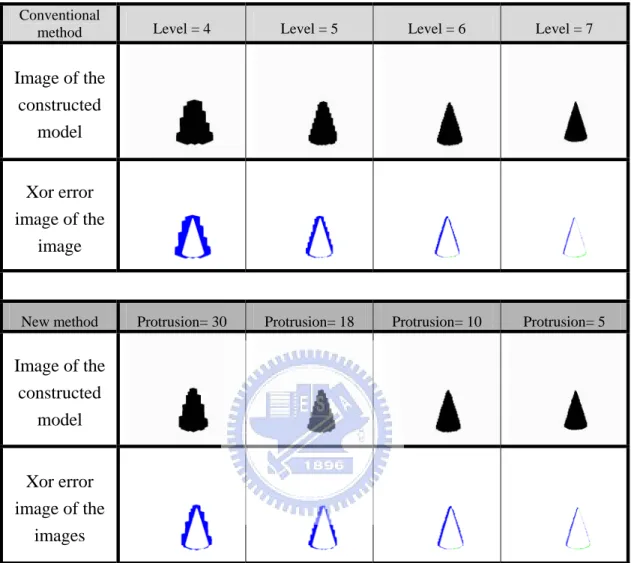
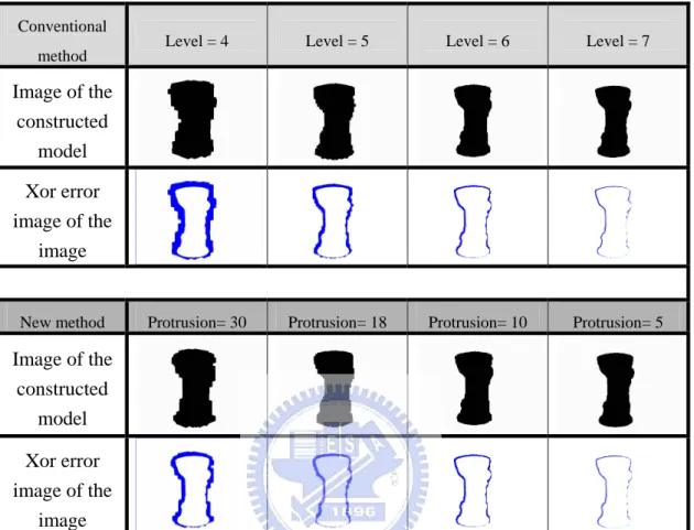
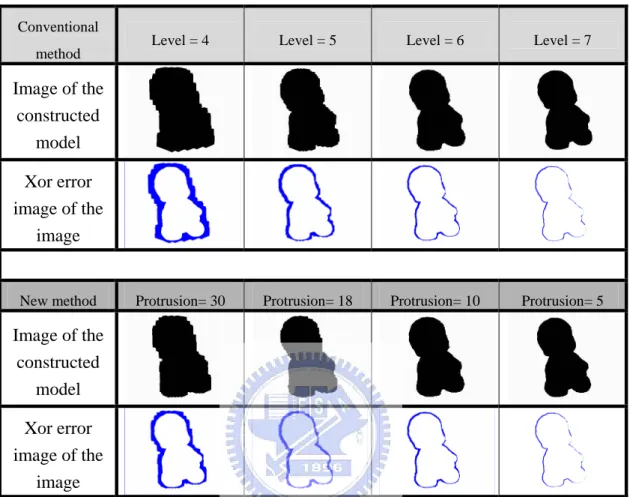
We list the numbers of all types of octants generated at each subdivision level, together with the projection error upper bound value and the quality index of the final constructed models in Table 2.8 to Table 2.13. In addition, the graphical display of the constructed object models and the XOR error images obtained by the conventional method and the new method are shown in Fig. 2.13 to Fig. 2.15.
(a) (b) (c)
Fig. 2.11. Three real objects used in the experiments: (a) a cone, (b) a vase, and (c) a boy sculpture.
(a) (b) (c)
Fig. 2.12. New views generated from the constructed octree models for (a) a cone, (b) a vase, and (c) a boy sculpture. The octree models are converted to VRML format and rendered using Cosmo© player.
Table 2.8. Numbers of black, grey, and white nodes of the cone generated by the conventional octree construction method with a fixed subdivision level.
Level=4 Level=5 Level=6 Level=7
Xor=116647 Xor= 53225 Xor=23682 Xor=9660
B GB GG W B GB GG W B GB GG W B GB GG W 0 0 - 1 0 0 - 1 0 0 - 1 0 0 - 1 0 1 0 - 7 1 0 - 7 1 0 - 7 1 0 - 7 1 2 0 - 8 48 0 - 8 48 0 - 8 48 0 - 8 48 3 0 - 32 32 0 - 32 32 0 - 32 32 0 - 32 32 4 4 - 108 144 4 - 108 144 4 - 108 144 4 - 108 144 5 84 - 393 387 84 - 393 387 84 - 393 387 6 609 - 1401 1134 609 - 1401 1134 7 3401 - 3349 4458 8
Table 2.9. Numbers of black, grey-black, grey-grey, and white nodes of the cone generated by our octree construction method with a specified projection error bound.
Protrusion=30 Protrusion=18 Protrusion=10 Protrusion=5 Xor=67123 Xor=44365 Xor=23685 Xor=9283
B GB GG W B GB GG W B GB GG W B GB GG W 0 0 0 1 0 0 0 1 0 0 0 1 0 0 0 1 0 1 0 0 7 1 0 0 7 1 0 0 7 1 0 0 7 1 2 0 0 8 48 0 0 8 48 0 0 8 48 0 0 8 48 3 0 1 31 32 0 0 32 32 0 0 32 32 0 0 32 32 4 2 54 48 144 4 26 82 144 4 9 99 144 4 4 104 144 5 0 61 0 323 1 213 55 387 31 137 237 387 54 59 332 387 6 0 7 0 433 7 762 0 1134 199 552 771 1134 7 122 1494 242 4310 8 1 0 0 1935
Table 2.10. Numbers of black, grey, and white nodes of the vase generated by the conventional octree construction method with a fixed subdivision level.
Level=4 Level=5 Level=6 Level=7
Xor=289493 Xor=144377 Xor=68356 Xor=30069
B GB GG W B GB GG W B GB GG W B GB GG W 0 0 - 1 0 0 - 1 0 0 - 1 0 0 - 1 0 1 0 - 8 0 0 - 8 0 0 - 8 0 0 - 8 0 2 0 - 41 23 0 - 41 23 0 - 41 23 0 - 41 23 3 1 - 133 194 1 - 133 194 1 - 133 194 1 - 133 194 4 88 - 532 444 88 - 532 444 88 - 532 444 88 - 532 444 5 685 - 2074 1497 685 - 2074 1497 685 - 2074 1497 685 - 2074 1497 6 3811 - 7482 5299 3811 - 7482 5299 7 17526 - 21460 20870 8
Table 2.11. Numbers of black, grey-black, grey-grey, and white nodes of the vase generated by our octree construction method with a specified projection error bound.
Protrusion=30 Protrusion=18 Protrusion=10 Protrusion=5
Xor=178926 Xor=118666 Xor=68365 Xor=28185
B GB GG W B GB GG W B GB GG W B GB GG W 0 0 0 1 0 0 0 1 0 0 0 1 0 0 0 1 0 1 0 0 8 0 0 0 8 0 0 0 8 0 0 0 8 0 2 0 0 41 23 0 0 41 23 0 0 41 23 0 0 41 23 3 1 17 116 194 1 8 125 194 1 1 132 194 1 0 133 194 4 12 284 188 444 40 151 365 444 81 76 455 444 88 32 500 444 5 0 316 0 1188 3 1137 283 1497 180 808 1155 1497 441 359 1703 1497 6 0 68 0 2196 1 3940 0 5299 1301 3100 3924 5299 7 496 8233 2489 20174 8 7 0 0 19905
Table 2.12. Numbers of black, grey, and white nodes of the boy sculpture generated by the conventional octree method with a fixed subdivision level.
Level=4 Level=5 Level=6 Level=7
Xor=366074 Xor=186064 Xor=89866 Xor=41534
B GB GG W B GB GG W B GB GG W B GB GG W 0 0 - 1 0 0 - 1 0 0 - 1 0 0 - 1 0 1 0 - 8 0 0 - 8 0 0 - 8 0 0 - 8 0 2 0 - 51 13 0 - 51 13 0 - 51 13 0 - 51 13 3 7 - 232 169 7 - 232 169 7 - 232 169 7 - 232 169 4 206 - 957 693 206 - 957 693 206 - 957 693 206 - 957 693 5 1483 - 3738 2435 1483 - 3738 2435 1483 - 3738 2435 6 7307 - 13437 9160 7307 - 13437 9160 7 31273 - 40955 35265 8
Table 2.13. Numbers of black, grey-black, grey-grey, and white nodes of the boy sculpture generated by our octree construction method with a specified projection error bound.
Protrusion=30 Protrusion=18 Protrusion=10 Protrusion=5
Xor=226886 Xor=156235 Xor=89872 Xor=37350
B GB GG W B GB GG W B GB GG W B GB GG W 0 0 0 1 0 0 0 1 0 0 0 1 0 0 0 1 0 1 0 0 8 0 0 0 8 0 0 0 8 0 0 0 8 0 2 0 0 51 13 0 0 51 13 0 0 51 13 0 0 51 13 3 7 46 186 169 7 16 216 169 7 10 222 169 7 4 228 169 4 19 476 300 693 103 325 607 693 133 159 291 693 174 69 888 693 5 0 438 0 1962 6 1927 488 2435 415 1443 2035 2435 955 717 2997 2435 6 0 166 0 3738 13 7107 0 9160 2139 5531 6966 9160 7 822 14814 5743 34349 8 54 0 0 45890
Conventional
method Level = 4 Level = 5 Level = 6 Level = 7
Image of the constructed model Xor error image of the image
New method Protrusion= 30 Protrusion= 18 Protrusion= 10 Protrusion= 5
Image of the constructed model Xor error image of the images
Fig. 2.13. The comparison between construction results of the cone obtained by the conventional method and the new method.
Conventional
method Level = 4 Level = 5 Level = 6 Level = 7
Image of the constructed model Xor error image of the image
New method Protrusion= 30 Protrusion= 18 Protrusion= 10 Protrusion= 5
Image of the constructed model Xor error image of the image
Fig. 2.14. The comparison between construction results of the vase obtained by the conventional method and the new method.
Conventional
method Level = 4 Level = 5 Level = 6 Level = 7
Image of the constructed model Xor error image of the image
New method Protrusion= 30 Protrusion= 18 Protrusion= 10 Protrusion= 5
Image of the constructed model Xor error image of the image
Fig. 2.15. The comparison between construction results of the boy sculpture obtained by the conventional method and the new method.
From the above tables the two methods can be compared in terms of memory storage, computation time, and the quality of the construction. Since the object model is represented by the leaf nodes of the constructed octree including black nodes and grey-black nodes, if available, the memory space required to store the constructed object model is proportional to the total number of black and grey-black nodes. On the other hand, the computer processing time required is mainly proportional to the entire set of leaf and internal nodes generated. Finally, the quality of the construction result is evaluated based on the XOR projection error given by the “Quality_Index”.
The following interesting observations can be made from the above experimental results:
(1) Based on the quality of the constructed object models expressed by the XOR value we can rank the construction results obtained by both the conventional and the new methods. For instance, from Tables 2.8 and 2.9, the ascending quality order of the construction results can be found to be < < < < = < < , where the symbol denotes the object model obtained by the conventional method with a maximum level parameter L, and the symbol denotes the result obtained by the new method with a projection error upper bound parameter P. C V4 V30N V5C V18N V6C N V10 V7C V5P VLC N P V
(2) During the construction process the generation patterns of the white nodes by the two methods are identical. To be more specific, the white nodes at a lower subdivision level must be completely generated before any white node can be generated at the next higher subdivision level. For instance, in Table 2.9 the full set of 1134 white nodes must be generated at level 6 before any white node at
level 7 is generated when the error control parameter P decreases from 18, 10, to 5.
(3) For the same quality of the construction results produced by the conventional and new methods the total leaf node number of the object model generated by the conventional method is greater than that generated by the new method. For instance, in Tables 2.8 and 2.9 the total leaf node number of is smaller than that of . The same observations can be also found in Tables 2.10 to 2.13.
N
V10
C
V6
(4) Under the assumption of the same or equivalent construction quality, the total internal and leaf nodes is less in the new method.
The observations (3) and (4) indicate that the new method takes less memory space and computation time to achieve the same construction quality when compared to the conventional method. These findings are plotted in Figures 2.16 to 2.17. In these plots a linear interpolation of the discrete set of construction results is made. Since the colors of the octants in the two methods are classified as three colors (White, Grey, and Black) and four colors (White, Grey-Grey, Grey-Black, and Black), respectivly, it is sufficient to use two bits to represent the color of the octant in the two methods. Let numc and numn be the total numbers of octants generaed in the conventional method and our new method. Then the total memory space in bits required for the two methods are numc*2 and numn*2, respectively. Since numn is less
than numc, as shown in the later section. We can conclude that the total memory space requirement in bit representation for our new method is less than that of the conventaional method.