國
立
交
通
大
學
應用數學系
碩
士
論
文
有界面活性劑之軸對稱界面在不同黏滯性之流體模擬
Axisymmetric Interfaces with insoluble surfactant in Navier-Stokes flow
with different viscosity
研 究 生:楊承翰
有界面活性劑之軸對稱界面在不同黏滯性之流體模擬
Axisymmetric Interfaces with insoluble surfactant in Navier-Stokes flow
with different viscosity
研 究 生:楊承翰 Student:Cheng-Han Yang
指導教授:賴明治 Advisor:Ming - Chih Lai
國 立 交 通 大 學
應 用 數 學 系
碩 士 論 文
A Thesis
Submitted to Department of Applied Mathematics College of Science
National Chiao Tung University in partial Fulfillment of the Requirements
for the Degree of Master
in
Applied Mathematics
June 2010
有界面活性劑之軸對稱界面在不同黏滯性之流體模
擬
學生:
楊承翰指導教授
:賴明治國立交通大學應用數學學系﹙研究所﹚碩士班
摘
要
本論文把 Immersed boundary method 發展到軸對稱圓柱座標系中來模擬液滴
在不可壓縮流中,液滴內外不同的黏滯度是我們所關心的。為方便分佈界面所產
生的力至流體以及內插流體流速至界面的移動速度,須藉由 Dirac delta function
將 Eulerian 流體和 Lagrangian 界面變數合併。我們使用 semi-implicit
second-order projection method 來解 Navier-Stokes 方程式並且利用 Indicator
function 來更新密度和黏滯度。把液滴放入流場中,觀察有加表面活性劑與沒加
表面活性劑的差異性。表面活性劑會分佈在界面中,並且影響表面張力的大小。
上述的方程式,我們皆加入人工速度去調整界面上網格的位置,使其分佈均勻。
Axisymmetric Interfaces with insoluble
surfactant in Navier-Stokes flow with different
viscosity
student:
Cheng-Han YangAdvisors:Dr.
Ming-Chih LaiDepartment﹙Institute﹚of
Applied MathematicsNational Chiao Tung University
ABSTRACT
In this study, the simulation of drop deformation in incompressible flow was executed
by developing an immersed boundary method in the axisym metric cylindrical
coordinates. The viscosity difference between two sides of
drop interface was
particularly considered in this paper. We implemented a semi-implicit second-order
projection scheme to solve Navier-Stokes equations. Various viscosity between two
sides of drop were tested on simulation, as well as the effect of the surfactant on drop,
which affect the surface tension. In addition, the distribution of marker positions were
stabilized by imposing the artificial velocity and compared to the original manner
without imposition of artificial velocity.
誌
謝
本篇論文的完成,首先要感謝我的指導教授 ─ 賴明治老師。在老師的細心
指點之下,讓我一點一滴熟悉數值偏微分方程以及科學計算的方法。我也從自己
的研究中找到對數值偏微分方程以及科學計算這塊領域的興趣與成就感。除了指
導教授外,在我們科學計算研究室中的其他學長們也給了我很多的幫助。感謝陳
冠羽學長在我剛踏入這塊領域時,指導我撰寫程式語言時所遇到的困難以及課業
上的問題。感謝黃仲尹學長與胡偉凡學長很有耐心地教我流體力學的相關理論以
及使用 Immersed boundary method 時會碰到的疑難雜症。
在論文口試期間,承蒙吳金典教授與黃聰明教授費心審閱並提供許多寶貴意
見,使得本論文變得更加完備,學生永遠銘記在心。
平常除了做數值計算研究外,我也要感謝同一屆的同學們與研究室的學長
們,他們與我一起打球,分享彼此的興趣,還有其他好朋友的陪伴如: SFD、GGC
讓我的研究生生活多采多姿,處處充滿著樂趣。
最後,我要好好地感謝我的家人,是他們鼓勵並支持著我做研究的興趣,讓
我可以無所顧忌地完成我的學業。希望能與他們,以及在我身邊所有關心我的
人,一起分享這篇論文完成的喜悅與榮耀。
目
錄
中文提要
………
i
英文提要
………
ii
誌謝
………
iii
目錄
………
iv
一、
Introduction ………
1
二、
The governing equations ………
2
2.1
Immersed boundary formulation ………
3
2.2
Surfactant concentration equation ………
5
2.3
Controlling the interfacial markers uniformly …
6
2.4
Density and viscosity equations ………
7
三、
Numerical method ………
8
四、
Numerical results ………
14
4.1
Convergent test ………
14
4.2
Oscillating drop ………
16
4.3
Effects of the clean drop deformation on the
Viscosity ………
18
4.4
Effects of the drop deformation on surfactant …
22
4.5
Effects of the drop deformation on Peclet number
26
五、
Conclusion ………
27
1
Introduction
The immersed boundary method was first used in reference to the method devel-oped by Peskin (1972) to simulate cardiac mechanics and associated blood flow. In this paper, we used this method to simulate the behavior of drop in extensional flow using Navier-Stoke equations in cylindrical geometries, where axisymmetric case was performed for convenience of computation. Numerous research has been studied in the subject as above. We attempted to resolve Navier-Stokes equations with various viscosity and density of a drop. Furthermore, we consider the case that surfactant was added on the interface and surfactant, such as soap, detergent, will impact the strength of surface extension.
We first consult [6] and [7] in order to transform the immersed boundary formulation [5] in three-dimensional coordinates into the cylindrical coordinates. Then, we must set the boundary conditions on r = 0 such as ur = 0 and ∂uz/∂r = 0
[6] for our study in the axisymmetric cylindrical coordinates. [5] presented the surfactant concentration equation in Lagrangian coordinates on the interface in the Cartesian coordinates. In order to examine a variety of axisymmetric cases, and according to [10], we should transform the equation into cylindrical coordinates for our study.
Since our initial velocity field has to satisfy Navier-Stokes equations and the axisymmetric boundary conditions, the uniaxial extensional flow ur = −0.5rG, uz =
zG[2] is an optimum. Surfactant on the drifts are flowing along (the direction of) the
fluid. Similarly, the flow (has) also affected the markers in Lagrangian coordinates on the interface. The following section will introduce a artificial method about marker redistribution.
The remaining sections of this paper are organized as follows. We present the governing equations in lagrangian coordinates on the interface which includes the immersed boundary formulas and the surfactant concentration equation in sec-tion 2. We imposed artificial velocities on some equasec-tions to modify the distance between markers. Since viscosity and density are variables in Navier-Stokes equa-tions, we update data of viscosity and density by indicator function. The numerical method which includes an algorithm of solving the Navier-Stokes equations, a mass conservative scheme for the surfactant equation and indicator function is described in section 3. In Section 4, we first examine the convergence of Navier-Stokes equa-tions , then we present the Oscillating drop and observe how much the drop volume leaks or bulks up. we emphasize the effects of the drop deformation on viscosity, surfactant and Peclet number P es, and observe the degree of deformation by [11].
2
The governing equations
In this paper, we consider an incompressible two-phase flow problem in a fixed three-dimensional cubic domain.The interface of the drop Σ separates two parts, Ω1
inside the interface and Ω2 outside the interface from our domain,which is a simple
closed surface immersed in the fluid. i.e.Ω = Ω1
S Ω2.
In each fluid region, the Navier-Stokes equations are satisfied as
ρi µ ∂ui ∂t + (ui· ∇) ui ¶ = ∇ · Ti+ ρig, in Ωi, (2.1) ∇ · ui = 0, in Ωi, (2.2) u = ub, in ∂Ω, (2.3)
where Ti = −piI + µi(∇ui+ ∇uTi ) is the stress tensor, pi is the pressure, ui is the
fluid velocity, ρi is the density, µi is the viscosity for i = 1, 2 in each fluid domain,
and g is the gravitational constant. The velocity is continuous across the interface Σ. Thus,
[u]Σ = u|Σ,2− u|Σ,1 = 0 (2.4)
and the normal stress jump is balanced by the interfacial force F (defined only on Σ) as
[Tn]Σ+ F = 0 (2.5)
where n is the unit normal vector on Σ directed towards fluid 2. In this paper, we use the immersed boundary method to approach the velocity solutions of the Navier-Stokes equations. The immersed boundary ( the interface ) exerts force F to the fluids and moves with local fluid velocity. For simplicity, gravity is neglected, so the same density of drop is only considered in this study. i.e. ρ1 = ρ2 = ρ.
To be convenient for calculation, our numerical experiment in the single phase was computed by non-dimensionlizing the following three dimensional equations,
ρ µ ∂u ∂t + (u · ∇) u ¶ = −∇p + ∇ · (2µE) + f, (2.6) ∇ · u = 0, (2.7) ∂Γ ∂t + (∇s· u) Γ = Ds∇ 2 sΓ, (2.8)
where u is the velocity, p is the pressure, ρ is the density, µ is the viscosity, Γ is the surfactant concentration, Ds is diffusivity, and E = (∇u + ∇uT)/2 is the rate
of deformation tensor.
Assume the dimensionless numbers, x = r0x∗, u = U∞u∗, µ = µ0µ∗, ρ = ρ0ρ∗,
equations are presented as follows. ρ∗ µ ∂u∗ ∂t∗ + (u ∗· ∇∗) u∗ ¶ = −∇∗p∗+ 1 Re∇ ∗ · (2µ∗E∗) + r0f0 ρ0U∞2 f∗, (2.9) ∇∗· u∗ = 0, (2.10) ∂Γ∗ ∂t∗ + (∇ ∗ s· u∗) Γ∗ = 1 P es ∇∗2 s Γ∗, (2.11)
where Re = ρ0U∞r0/µ0 and P es = r0U∞/Ds. In the axisymmetric cylindrical
coordinates, we spread the interfacial force into fluid by Dirac delta function δ(x) =
δ(r)δ(z) as follows.
f (x, t) = Z
Σ
F (s, t) δ (x − X (s, t)) ds,
where x = (r, z) is the fluid position, X (s, t) = (R (s, t) , Z (s, t)) is the interfacial position, s is the interfacial parameter, F is the interfacial force, σ is the surface tension, and Σ is the domain of parameter.
Assume the dimensionless number σ = σ0σ∗, Ca = µ0U∞/σ0, then we can get
ρ∗ µ ∂u∗ ∂t∗ + (u ∗· ∇∗) u∗ ¶ = −∇∗p∗+ 1 Re∇ ∗· (2µ∗E∗) + 1 ReCaf ∗ (2.12) ∇∗· u∗ = 0, (2.13) ∂Γ∗ ∂t∗ + (∇ ∗ s· u∗) Γ∗ = 1 P es ∇∗2 s Γ∗. (2.14)
The operator forms of governing equaitons in the acisymmetric cylindrical coordintates will be introduced on the following sections. In fact, the characteristic velocity
U∞= Gr0 where G is the principle strain rate and 2r0 is the equivalent diameter of
the drop. Hence, we have Re = ρ0(Gr0)r0/µ0, Ca = µ0Gr0/σ0, and P es = r0U∞/Ds.
2.1
Immersed boundary formulation
In every corner of this paper, we consider the Navier-Stokes equations in cylin-drical coordinates instead of Cartesian coordinates,in addition the domain is ax-isymmetric. Hence, it is convenient to compute our data in a cylindrical coordinate system (r, θ, z). Because of axisymmetric, domain is azimuthal symmetry and the flow depends spatially on only two cylindrical coordinates (r, z). The interface Σ is represented by a parametric form (r(s, t), z(s, t)), 0 ≤ s ≤ Lb, where s is the
parameter of the initial configuration of the interface, which is not necessarily the arc-length.
The following governing equations can be expressed in the usual immersed bound-ary formulation using the non-dimenionlization process.
ρ µ ∂ur ∂t + ur ∂ur ∂r + uz ∂ur ∂z ¶ + ∂p ∂r = 1 Re ½ 1 r ∂ ∂r µ 2µr∂ur ∂r ¶ + ∂ ∂z · µ µ ∂ur ∂z + ∂uz ∂r ¶¸ − 2µur r2 ¾ + 1 ReCafr, (2.15) ρ µ ∂uz ∂t + ur ∂uz ∂r + uz ∂uz ∂z ¶ + ∂p ∂z = 1 Re ½ 1 r ∂ ∂r · µr µ ∂ur ∂z + ∂uz ∂r ¶¸ + ∂ ∂z µ 2µ∂uz ∂z ¶¾ + 1 ReCafz, (2.16) 1 r ∂rur ∂r + ∂uz ∂z = 0, (2.17) f (x, t) = Z Σ F (s, t) δ (x − X (s, t)) ds, (2.18) ∂X (s, t) ∂t = U (s, t) = u (X (s, t) , t) = Z Ω u (x, t) δ (x − X (s, t)) dx, (2.19) F (s, t) = ∂ ∂s(σ (s, t) τ (s, t)) − 1 R ∂Z ∂s (τ (s, t) n) , (2.20) τ (s, t) = ∂X ∂s ¯ ¯∂X ∂s ¯ ¯ = (Rs, Zs) p R2 s+ Zs2 , (2.21) n = p(Zs, −Rs) R2 s+ Zs2 . (2.22) Here, u = (ur, uz) is the velocity of the fluid,( ur is the radial velocity and uz is the
axial velocity), U = (Ur, Uz) is the velocity of the drop , σ is the surface tension, τ
is the unit tangent vector on the interface,and n is the outward normal vector on the interface. The dimensionless numbers are Reynolds number and Capillary number, respectively. The Reynolds number (Re) describing the ratio between the inertial force and the viscous force.The capillary number (Ca) describing the strength of the surface tension. The Eq.(2.17) is the divergence free equation which means continuity. we get the force f = (fr, fz) on the fluid by the Eq.(2.18). Because the
Eq.(2.18) represents the interfacial force F spreads to the fluid, and the force F on the interface is balanced by the normal stress. The Eq.(2.19) represents the interface was moved by the fluid velocity. The Eulerian (x) and Lagrangian (X) variable are used in the three-dimensional Dirac delta function δ(x) = δ(r)δ(z).The Eq.(2.20) represents the interfacial force F which arises from the surface tension and its form is derived from Laplace-Young condition.
We consider the case that the drop is contaminated by the surfactant. Let the interface be contaminated by the surfactant, which reduces the surface tension, so that we can find the phenomenon that the surface tension is smaller as the surfactant concentration is higher. The relation between surface tension and surfactant concen-tration can be described by the linear equation. The following is the approximation of linear equation.
σ (Γ) = σc(1 − βΓ) , (2.23)
where Γ is the surfactant concentration, σcis the surface tension of a clean interface,
and β is a dimensionless number that measures the sensitivity of surface tension to variation in surfactant concentration.
2.2
Surfactant concentration equation
Since we want to close the system, the surfactant is insoluble to the buck fluids such that it is convected and diffused along the interface. Hence, there is no exchange between the interface and the bulk fluids. Due to those reasons, the total mass of the surfactant must be conserved. The equation of surfactant concentration is derived in this subsection. In the three dimensional cylindrical coordinates, we present a slightly different derivation from Stone [9] for the surfactant transport equation in order to make the total mass of the surfactant conserved.
We can regard the surface as the curve in r-z coordinates in the case of ax-isymmetric cylindrical coordinates. So, let L(t) be an interfacial segment where the surfactant concentration (the mass of the surfactant per unit surface area) is defined. Since the surfactant on the material element don’t transport nor spread to the surrounding (bulk) fluids, the mass on the segment remained consistent.
Hence, d dt Z L(t) Γ (l, t) Rdl = 0, (2.24) where dl is the arc-length element. In order to apply the time derivative more easily, we rewrite the above equation in terms of the initial parameter s as
d dt Z L(0) Γ (s, t) ¯ ¯ ¯ ¯∂X∂s ¯ ¯ ¯ ¯ Rds = 0. (2.25) Further we take the time derivative inside the integral,
Z L(0) µ ∂Γ ∂t ¯ ¯ ¯ ¯∂X∂s ¯ ¯ ¯ ¯ R + Γ∂t∂ µ¯¯ ¯ ¯∂X∂s ¯ ¯ ¯ ¯ R ¶ ¶ ds = 0. (2.26)
Note that, the interface and surfactant concentration are tracked in a Lagrangian manner in our present formulation. Thus, the time derivative of the first term in
Eq.(2.26) is exactly the material derivative of Stones derivation. Now we need to compute the rate of the stretching factor, and using Eq.(2.19), we have
∂ ∂t µ ¯¯ ¯ ¯∂X∂s ¯ ¯ ¯ ¯ R ¶ = ∂R ∂t ¯ ¯ ¯ ¯∂X∂s ¯ ¯ ¯ ¯ + R∂t∂ ¯ ¯ ¯ ¯∂X∂s ¯ ¯ ¯ ¯ = Ur ¯ ¯ ¯ ¯∂X∂s ¯ ¯ ¯ ¯ + R ∂R ∂s ∂s∂ ¡∂R ∂t ¢ +∂Z ∂s ∂s∂ ¡∂Z ∂t ¢ ¯ ¯∂X ∂s ¯ ¯ = Ur ¯ ¯ ¯ ¯∂X∂s ¯ ¯ ¯ ¯ + R ∂R ∂s ∂U∂sr¯+∂Z∂s ∂U∂sz ¯∂X ∂s ¯ ¯ (2.27) = Ur ¯ ¯ ¯ ¯∂X∂s ¯ ¯ ¯ ¯ + R ∂R ∂s ¡ ∇Ur· ∂X∂s ¢ +∂Z ∂s ¡ ∇Uz· ∂X∂s ¢ ¯ ¯∂X ∂s ¯ ¯ = Ur ¯ ¯ ¯ ¯∂X∂s ¯ ¯ ¯ ¯ + µ ∂U ∂τ · τ ¶ R ¯ ¯ ¯ ¯∂X∂s ¯ ¯ ¯ ¯ = (∇s· u) R ¯ ¯ ¯ ¯∂X∂s ¯ ¯ ¯ ¯ .
Where, the notation ∇s· u means the surface divergence in axisymmetric cylindrical
coordinates and ∇s·u = Ur/R+(∂U/∂τ )·τ . Since the material segment is arbitrary,
we can get R ¯ ¯ ¯ ¯∂X∂s ¯ ¯ ¯ ¯∂Γ∂t + R ¯ ¯ ¯ ¯∂X∂s ¯ ¯ ¯ ¯ ( ∇s· u ) Γ = 0. (2.28)
If we permit surfactant diffusion along the interface, we obtain the surfactant transport-diffusion equation as R ¯ ¯ ¯ ¯∂X∂s ¯ ¯ ¯ ¯∂Γ∂t + r ¯ ¯ ¯ ¯∂X∂s ¯ ¯ ¯ ¯ ( 5s· u ) Γ = 1 P es ∂ ∂s " µ R ∂Γ ∂s ¶ , ¯¯ ¯ ¯∂X∂s ¯ ¯ ¯ ¯ # (2.29)
where P es (Peclet number) is a dimensionless number relevant in the study of
trans-port phenomena in fluid flows and the boundary condition of Γ is ∂Γ/∂s = 0 on
∂L (t) . We note that surface diffusion is also written in terms of initial parameter s.
2.3
Controlling the interfacial markers uniformly
The interface might be deformed as a velocity field in the domain, which causes our computational markers on the interface to concentrate on some part of interface along the fluid flowing direction. This phenomenon leads into a larger error on the drop volume than the one which interfacial markers are uniformly distributed.
Since drop deformation is only related to the force in the normal direction, we impose an artificial velocity on Eq.(2.19) to redistribute the interfacial markers uni-formly. Hence, substitute Eq.(2.19) into
∂X (s, t) ∂t = U (s, t) + U a(s, t) τ = u (X (s, t) , t) + Ua(s, t) τ = Z Ω u (x, t) δ (x − X (s, t)) dx + Ua(s, t) τ , (2.30)
where the scalar Ua is the artificial velocity, and it can modify the marker
posi-tions such that they avoid being moved by the tangential force. This condition
∂ |∂X/∂s| /∂s = 0 means that the tangential displacement of markers remains
un-changed. According to those conditions, we obtain
Ua(s, t) − Ua(0, t) = s 2π Z 2π 0 ∂U ∂s0 · τ 0ds0− Z s 0 ∂U ∂s0 · τ 0ds0, (2.31)
where Ua(0, t) = 0, since we should fix one marker to modify their relative positions.
The new marker positions have changed after adding the artificial velocity term, so Eq.(2.29) has to add some term to preserve that the equation holds. The following is the modified surfactant transport-diffusion equation,
R ¯ ¯ ¯ ¯∂X∂s ¯ ¯ ¯ ¯∂Γ∂t + R ¯ ¯ ¯ ¯∂X∂s ¯ ¯ ¯ ¯ ( 5s· u ) Γ − ∂ ∂s(RU aΓ) = 1 P es ∂ ∂s " µ R∂Γ ∂s ¶ , ¯¯ ¯ ¯∂X∂s ¯ ¯ ¯ ¯ # . (2.32)
2.4
Density and viscosity equations
Because the drop formation would change as fluid flows by, we have to update the viscosity and density of domain, including inside and outside of the drop, need to be updated using indicator function.
I (x, t) =
Z
Ω
δ (x − X) dX,
Then, we take gradient to both side to obtain, OI (x, t) = O Z Ω δ (x − X) dX, = Z Ω Oδ (x − X) dX , = − Z ∂Ω n · δ (x − X) ds
Furthermore, we take divergence to both side to obtain, O · OI (x, t) = −O · Z ∂Ω n · δ (x − X) ds (2.33) Moreover, ρ (x, t) = ρ2+ (ρ1− ρ2) I (x, t) , (2.34) µ (x, t) = µ2+ (µ1− µ2) I (x, t) (2.35)
3
Numerical method
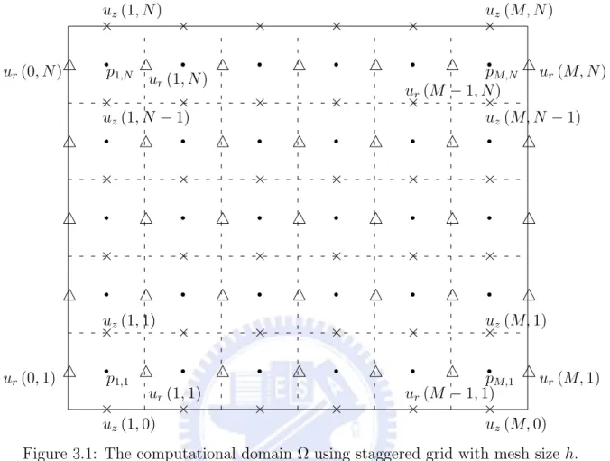
In this paper,computational solution of the fluid flow variables are defined on a staggered grid. This implies that different dependent variables are evaluate at different grid points.
More specifically, the pressure is defined on the grid points labelled as x = (ri−1/2, zj−1/2) = ((i − 1/2)h, (j − 1/2)h) for i = 1, 2, . . . , M, j = 1, 2, . . . , N, the
velocity components ur and uz are defined at (ri+1/2, zj) = (ih, (j − 1/2)h),for
i = 1, 2, . . . , M − 1, j = 1, 2, . . . , N and (ri, zj+1/2) = ((i − 1/2)h, jh),for i =
1, 2, . . . , M, j = 1, 2, . . . , N − 1,respectively, where the spacing h = ∆r = ∆z. In addition, the positions of density and viscosity are the same with those of pressure. A accepted staggered grid configuration is shown in Fig.3.1.It can be seen that pres-sures are defined at the center of each cell while velocity components are defined at the center of the call faces.
For the immersed interface, we use a collection of discrete points sk = k∆s, k =
1, 2, . . . , MK such that the Lagrangian markers are denoted by X = X(sk) =
(Rk, Zk). The surfactant concentration Γk and surface tension σk are defined at
the half-integer points given by sk−1/2 = (k − 1/2)∆s. Without loss of generality,
for any function defined on the interface φ(s), we approximate the partial derivative
∂φ/∂s by
Dsφ (s) =
φ (s + ∆s/2) − φ (s − ∆s/2)
∆s . (3.1) Since |DsXk| can approximate the interface stretching factor by using this finite
difference convention, the unit tangent vector τk are defined at the half-integer
points.
Let ∆t be the time step size, and n be the superscript time step index. At the beginning of each time step, e.g., step n, the variables Xnk = X (sk, n∆t) , Γnk =
Γ¡sk−1/2, n∆t
¢
, un = u (x, n∆t), and pn = p (x, n∆t) are all given. The details of
r r r r r r r r r r r r r r r r r r r r r r r r r r r r r r 4 4 4 4 4 4 4 4 4 4 4 4 4 4 4 4 4 4 4 4 4 4 4 4 4 4 4 4 4 4 4 4 4 4 4 × × × × × × × × × × × × × × × × × × × × × × × × × × × × × × × × × × × × ur(0, 1) ur(1, 1) ur(M − 1, 1) ur(M, 1) ur(0, N) u r(1, N) ur(M, N ) ur(M − 1, N ) uz(1, 0) uz(1, 1) uz(1, N − 1) uz(1, N ) uz(M, 0) uz(M, 1) uz(M, N − 1) uz(M, N ) p1,1 pM,1 p1,N pM,N
Figure 3.1: The computational domain Ω using staggered grid with mesh size h.
1. Surface tension and unit tangent vector
Compute the surface tension and unit tangent vector on the interface as
σn k = σc(1 − βΓnk) , (3.2) τnk = DsX n k |DsXnk| , (3.3) both of which hold for sk−1/2 = (k − 1/2)∆s. Then we define the interfacial
force as Fn k = Ds(σknτnk) − DsZkn Rn k (τn knnk) , (3.4) at point Xk.
2. Force to the fluid
Distribute the force from the markers to the fluid by fn(x) =X
k
where the smooth version of Dirac delta function, δh(x) = ½ 1 4h ¡ 1 + cos¡πx 2h ¢¢ , if −2h ≤ x ≤ 2h 0, otherwise, (3.6) is used. 3. Navier-Stokes equations
Solve the Navier-Stokes equations. This can be done by the following semi-implicit second-order projection scheme, where the nonlinear term is approxi-mated by a second-order extrapolation to avoid solving a nonlinear system at each time step.
ρn · 3 ˜urn+1− 4unr + un−1r 2∆t + µ 2un r ∂un r ∂r − u n−1 r ∂un−1 r ∂r ¶ + µ 2un z ∂un r ∂z − u n−1 z ∂un−1 r ∂z ¶¸ = −∂p n ∂r + 1 Re{ 2 r ∂ ∂r µ rµn∂ ˜urn+1 ∂r ¶ + ∂ ∂z µ µn∂unz ∂r ¶ + ∂ ∂z µ µn∂unr ∂r ¶ − 2µ nu˜ rn+1 r2 } + 1 ReCaf n r ρn · 3 ˜uzn+1− 4unz + un−1z 2∆t + µ 2un r ∂un z ∂r − u n−1 r ∂un−1 z ∂r ¶ + µ 2un z ∂un z ∂z − u n−1 z ∂un−1 z ∂z ¶¸ = −∂p n ∂z + 1 Re{ 1 r ∂ ∂r µ rµn∂ ˜uzn+1 ∂r ¶ +1 r ∂ ∂r µ rµn∂unr ∂z ¶ + 2 ∂ ∂z µ µn∂unz ∂z ¶ } + 1 ReCaf n z (3.7) ˜ u = ub, on ∂Ω, (3.8) ˜ ∇h · un+1 = 0, (3.9) ˜ ∇h· µ 1 ρn∇˜hφ n+1 ¶ = 3 ˜∇h· ˜u 2∆t , ∂φ ∂n = 0, on ∂Ω (3.10) ˜ ∇hφn+1 = 3ρn¡u˜n+1− un+1¢ 2∆t , (3.11) pn+1 = pn+ φn+1. (3.12)
Here the gradient operator ˜∇h = (∂/∂r, ∂/∂z) , the divergent operator ˜∇h· =
(1
r∂r∂r, ∂z∂)· and the Laplace operator
˜ ∆hu˜n+1= µ ∂2un+1 r ∂r2 + 1 r ∂un+1 r ∂r + ∂2un+1 r ∂z2 − un+1 r r2 , ∂2un+1 z ∂r2 + 1 r ∂un+1 z ∂r + ∂2un+1 z ∂z2 
˜ ∇2 hφn+1 = ∂2φn+1 ∂r2 + 1 r ∂φn+1 ∂r + ∂2φn+1 ∂z2
are the standard centered difference operator on the grid which is defined at the staggered grid mesh. One can see that the above Navier-Stokes solver involves solving two Helmholtz equations for velocity ˜un+1 and one Poisson
equation for pressure. These elliptic equations are solved by using the direct sparse solver which is provided by CXML.
4. Ghost values form boundary condition
The numercial experiment in next section is concerned with a drop in a extensional flow. In this case, the initial condition of a extensional flow u = G (−0.5r, z) is applied in the beginning. The velocity of the computational domain is [a, b] × [c, d] where a = 0 because of axisymmetric, and the bound-ary conditions of the velocities are ur = 0 and ∂uz/∂r = 0 on r = 0. That
is,ur(r, c) = −0.5rG, ur(r, d) = −0.5rG, ur(a, z) = 0, ur(b, z) = −0.5bG,and
uz(r, c) = cG, uz(r, d) = dG, uz(a, z) = zG, uz(b, z) = zG. Then
approxima-tions for ghost values from linear extrapolation are given in the following.
ur(i, 0) = −rG − ur(i, 1) , ur(i, N + 1) = −rG − ur(i, N ) , ur(0, j) = 0, ur(M, j) = −0.5bG; uz(i, 0) = cG, uz(i, N ) = dG, uz(0, j) = −uz(1, j) , uz(M + 1, j) = 2zG − uz(M, j) .
Note that ur(i, 1) , ur(i, N) , uz(1, j) , anduz(M + 1, j) are unknowns for the
system when these ghost values are used. Therefore, the effect of these ghost values will appear in the right-hand side of the linear system and simultane-ously affect the coefficients of the linear system.
5. Updating position of marks
Interpolate the new velocity on the fluid lattice points onto the marker points and move the marker points to new positions.
Un+1k = X
x
un+1δh(x − Xnk)h2, (3.13)
Xn+1
In order to redistribute the interfacial markers more uniformly, we should add the artificial velocity,
UAn+1 k = k∆s 2π M X k0=0 DsUn+1k · τn+1k ∆s − k X k0=0 DsUn+1k · τn+1k ∆s. (3.15)
From the above equations, we have the modified marker positions, Xn+1
k = Xnk+ ∆tUn+1k + ∆tUAn+1k τn+1k . (3.16)
6. Update surfactant concentration distributionΓn+1k
Since the surfactant is insoluble, the total mass on the interface must be con-served. Thus, it is important to develop a numerical scheme for the surfactant concentration equation to preserve the total mass. This can be done as follows. Substitute Eq.(2.27) of rate of stretching factor into the Eq.(2.29), we have
R ¯ ¯ ¯ ¯∂X∂s ¯ ¯ ¯ ¯∂Γ∂t +∂t∂ µ ¯¯ ¯ ¯∂X∂s ¯ ¯ ¯ ¯ R ¶ Γ = 1 P es ∂ ∂s " µ R∂Γ ∂s ¶ , ¯¯ ¯ ¯∂X∂s ¯ ¯ ¯ ¯ # (3.17)
Now we discretiz the above equation by the Crank-Nicholson scheme in a symmetric way as Γn+1 k − Γnk ∆t rkn+1¯¯DsXn+1k ¯ ¯ + Rn k|DsXnk| 2 + Rn+1k ¯¯DsXn+1k ¯ ¯ − Rn k|DsXnk| ∆t Γn+1 k + Γnk 2 = 1 P es 1 ∆s " Rn+1 k+1/2 |DsXn+1k+1| + |DsXn+1k | Γn+1 k+1 − Γn+1k ∆s − Rn+1 k−1/2 |DsXn+1k | + |DsXn+1k−1| Γn+1 k − Γn+1k−1 ∆s + R n k+1/2 ¯ ¯DsXnk+1¯¯ + |DsXnk| Γn k+1− Γnk ∆s − Rn k−1/2 |DsXnk| + ¯ ¯DsXnk−1¯¯ Γn k− Γnk−1 ∆s # (3.18) Where k is “half-integer” index, i.e. k = 0.5, 1.5, . . . , MK − 1/2. According
to the new interfacial marker position Xn+1
k obtained in the previous step and
the boundary condition (Γn+1
k − Γn+1k−1)/∆s = 0, where k = 0.5 or MK + 1/2,
on the endpoints of the interface, Eq.(3.18) results in a symmetric tri-diagonal linear system which can be solved easily. More importantly, the total mass of surfactant is conserved numerically; that is,
X k Γn+1 k |DsXn+1k |Rn+1k−1/2∆s = X k Γn k|DsXnk|Rnk−1/2∆s (3.19)
The summation in Eq.(3.19) is the mid-point rule discretization for the inte-gral in Eq.(2.25).The thing that the total mass is conserved can be derived
by taking the summation of both sides of Eq.(3.18) and using the boundary condition.
Note that, when the artificial velocity is imposed on our equations like Eq.(3.16), Eq.(3.18) also have to impose the artificial velocity as follows.
Γn+1 k − Γnk ∆t Rn+1 k ¯ ¯DsXn+1k ¯ ¯ + Rn k|DsXnk| 2 + Rn+1 k ¯ ¯DsXn+1k ¯ ¯ − Rn k|DsXnk| ∆t Γn+1 k + Γnk 2 − " Rn+1k+1/2UAn+1 k+1/2 ¡ Γn+1k+1 + Γn+1k ¢/2 − rn+1k−1/2UAn+1 k−1/2 ¡ Γn+1k + Γn+1k−1¢/2 2∆s +R n k+1/2UAnk+1/2 ¡ Γn k+1+ Γnk ¢ /2 − Rn k−1/2UAnk−1/2 ¡ Γn k + Γnk−1 ¢ /2 2∆s # = 1 P es 1 ∆s " Rn+1 k+1/2 |DsXn+1k+1| + |DsXn+1k | Γn+1 k+1 − Γn+1k ∆s − Rn+1 k−1/2 |DsXn+1k | + |DsXn+1k−1| Γn+1 k − Γn+1k−1 ∆s + R n k+1/2 ¯ ¯DsXnk+1¯¯ + |DsXnk| Γn k+1− Γnk ∆s − Rn k−1/2 |DsXnk| + ¯ ¯DsXnk−1¯¯ Γn k − Γnk−1 ∆s # . (3.20)
7. Update density and viscosity
Since the density and viscosity are discontinuous constants across the interface, they can be represented by Eq.(2.34)and Eg.(2.35). By Eq.(2.32) and Lapace operator in the cylindrical coordinates, we obtain
˜
∆hIi,j =
Ii+1,j − 2Ii,j+ Ii−1,j
∆r2 +
1
ri
Ii+1,j− Ii−1,j
2∆r +
Ii,j+1− 2Ii,j+ Ii,j−1
∆z2 , ∂I ∂n = 0, on ∂Ω = Gi+1/2,j− Gi−1/2,j ∆r + Gi,j ri + Gi,j+1/2− Gi−1,j−1/2 ∆z (3.21) where, Gi,j = µ Gi+1/2,j Gi,j+1/2 ¶ = P k n1 kdh ¡ ri+1/2,j− Rk ¢ dh(zi,j − Zk) dh∆s P k n2 kdh(ri,j − Rk) dh ¡ zi,j+1/2− Zk ¢ dh∆s
4
Numerical results
4.1
convergent test
First of all, we test the convergence of Navier-Stokes solver. Here, we perform different computations with varying meshes h = ∆r = ∆z = 1/32, 1/64, 1/128,and the time step size is ∆t = h/4.The solutions are computed up to time T = 1.The problem is set up in fluid domain Ω = [0, 1] × [−1, 1], the Reynolds number Re = 1
and the capillary number Ca = 1. We set exact solutions as follows and fr, fz obtain
by E.q.(2.15) ,E.q.(2.16). ur(r, z, t) = π 2r 3cos (πz) e−t uz(r, z, t) = r2(cos (πr) − 2sin (πz)) e−t p (r, z, t) = cos (2πr) cos (πz) e−t When, ρ (r, z, t) = 1 µ (r, z, t) = 1
Table 1: The mesh refinement analysis of the velocity ur, uz.
h kur− uexactk∞ Rate kuz − uexactk∞ Rate
1/32 4.6868E − 04 - 7.7483E − 04 -1/64 2.0812E − 04 1.1712 4.1138E − 04 0.9134 1/128 1.1699E − 04 0.8310 2.2038E − 04 0.9005 When, ρ (r, z, t) = (1.5 + cos (πr)) e−t µ (r, z, t) = 1
Table 2: The mesh refinement analysis of the velocity ur, uz.
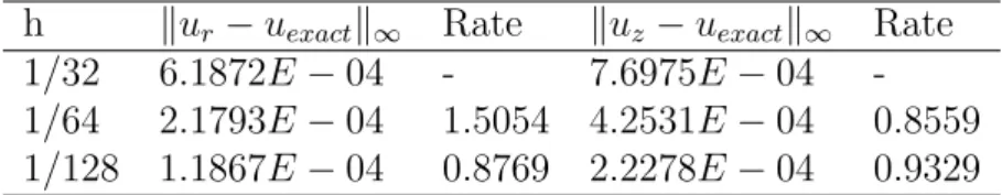
h kur− uexactk∞ Rate kuz − uexactk∞ Rate
1/32 6.1872E − 04 - 7.6975E − 04 -1/64 2.1793E − 04 1.5054 4.2531E − 04 0.8559 1/128 1.1867E − 04 0.8769 2.2278E − 04 0.9329
When,
ρ (r, z, t) = (1.5 + cos (πr)) e−t
µ (r, z, t) = ¡¡2r3− 3r2¢cos (πz) + 1¢e−t
Table 3: The mesh refinement analysis of the velocity ur, uz.
h kur− uexactk∞ Rate kuz − uexactk∞ Rate
1/32 6.3648E − 04 - 8.9644E − 04 -1/64 2.3356E − 04 1.4463 5.4650E − 04 0.7140 1/128 1.2293E − 04 0.9260 3.3458E − 04 0.7079
Table 3 shows the mesh refinement analysis of the velocity ur, uz. One can see
that the error decreases substantially when the mesh is refined, and the rate of con-vergence is somewhat first order. Note that, the fluid variables are defined at the staggered grid in r − z coordinates, but the density and viscosity are defined at the center of of the uniform grid. In addition there are some cross derivative terms in our equations, so it is not fully implicit. Thus it is why the rate of convergence behaves less than second-order.
After above test, we impose the surfactant on the interface to observe the drop behavior. We observe effects of the clean drop deformation on the viscosity in an extensional flow , ur = −0.5Gr and uz = Gz, where G is the principal strain
rate [6], and is chosen as G = 1. The computational domain is chosen as Ω = [0, 1] × [−1, 1] in the axisymmetrical cylindrical coordinates, and the initial drop is chosen as a circular one with radius r0 = 0.25. We choose β = 1 for the surface
tension equation Eq.2.23. In order to make our research convinced, we should carry out the convergence study of the immersed boundary method. We use the different mesh h = ∆r = ∆z = 1/32, 1/64, 1/128 and 1/256 to perform our computation relatively. The Lagrangian mesh is chosen as ∆s ≈ h and the time step size is ∆t = h/8. The solutions are computed up to time T = 1. Since it is not easy to obtain the analytical solution from our problem, we choose the finest mesh as our reference solution to compute the L∞ error between the reference solution and the
solution which is solved from the coarser grid. Here, we choose Reynolds number
Re = 1, Capillary number Ca = 0.25, Peclet number P es = 12.5, the viscosity
Table 4: The mesh refinement analysis of the velocity ur, uz, and the surfactant
concentration Γ.
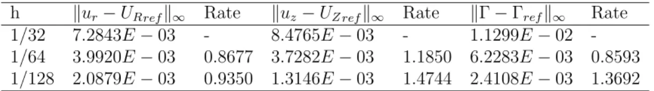
h kur− URrefk∞ Rate kuz− UZ refk∞ Rate kΓ − Γrefk∞ Rate
1/32 7.2843E − 03 - 8.4765E − 03 - 1.1299E − 02 -1/64 3.9920E − 03 0.8677 3.7282E − 03 1.1850 6.2283E − 03 0.8593 1/128 2.0879E − 03 0.9350 1.3146E − 03 1.4744 2.4108E − 03 1.3692
Table 4 shows that the error of kur− URrefk∞, kuz− UZ refk∞, and kΓ − Γrefk∞
converge to zero where URref, UZ ref, and Γref are r-axial, z-axial reference velocities,
and reference surfactant concentration relatively. The convergent rates for ur, uz,
and Γ are about first order, but our method is a second order scheme. Note that since the fluid velocities are defined at the staggered grid in r − z coordinates, the refined mesh will not coincide with the same grid locations. Thus, we approximate the coarser grid by cubic spline interpolation the velocities obtained from the reference grid near the coarser grid. In addition there are some cross derivative terms in our equations, so it is not fully implicit. We attribute this is part of the reason why the rate of convergence behaves less than second-order. Similarly, the surfactant concentration is defined at “half-integer” grid. When we average the reference grid, we should use the weighted average since the concentration is the mass per unit surface area.
4.2
Oscillating drop
Before to proceed, it is important to check how much the drop volume leaks or bulks up since it affects the computational accuracy. We test a simple case that a spheroid drop in the static liquid will be shrunk and turn into a sphere drop. This computational domain is set up as Ω = [0, 1] × [−1, 1] in the axisymmetrical cylindrical coordinates, and put a spheroid drop with the semi-major axis whose length is a = 3/4 and with the semi-minor axis whose length is b = 1/3, respectively into our domain. Then, given the computational mesh h = ∆r = ∆z, ∆t = h/8, the Reynolds number Re = 25, the Capillary number Ca = 0.04, and the surface Peclet number P es = 12.5. The initial surfactant concentration is uniformly distributed
along the interface such as Γ (0, s) = 0.5. The parameters in E.q.2.23 are chosen as
σc = 1 and β = 0.5,respectively. In the meanwhile, we consider the density inside
and outside of the drop are µ1 = 2 and µ2 = 1, respectively, and we computed the
relative error of the drop volume Ver by
Ver =
|V − Vi|
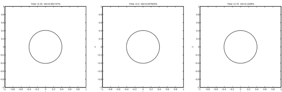
, where Vi = initial volume. −1 −0.8 −0.6 −0.4 −0.2 0 0.2 0.4 0.6 0.8 1 −1 −0.8 −0.6 −0.4 −0.2 0 0.2 0.4 0.6 0.8 1 r z Time =0 Ver=0% −1 −0.8 −0.6 −0.4 −0.2 0 0.2 0.4 0.6 0.8 1 −1 −0.8 −0.6 −0.4 −0.2 0 0.2 0.4 0.6 0.8 1 r z Time =0.25 Ver=0.017183% −1 −0.8 −0.6 −0.4 −0.2 0 0.2 0.4 0.6 0.8 1 −1 −0.8 −0.6 −0.4 −0.2 0 0.2 0.4 0.6 0.8 1 r z Time =0.5 Ver=0.023756% −1 −0.8 −0.6 −0.4 −0.2 0 0.2 0.4 0.6 0.8 1 −1 −0.8 −0.6 −0.4 −0.2 0 0.2 0.4 0.6 0.8 1 r z Time =0.75 Ver=0.040887% −1 −0.8 −0.6 −0.4 −0.2 0 0.2 0.4 0.6 0.8 1 −1 −0.8 −0.6 −0.4 −0.2 0 0.2 0.4 0.6 0.8 1 r z Time =1 Ver=0.0554% −1 −0.8 −0.6 −0.4 −0.2 0 0.2 0.4 0.6 0.8 1 −1 −0.8 −0.6 −0.4 −0.2 0 0.2 0.4 0.6 0.8 1 r z Time =1.25 Ver=0.070361% −1 −0.8 −0.6 −0.4 −0.2 0 0.2 0.4 0.6 0.8 1 −1 −0.8 −0.6 −0.4 −0.2 0 0.2 0.4 0.6 0.8 1 r z Time =1.5 Ver=0.074612% −1 −0.8 −0.6 −0.4 −0.2 0 0.2 0.4 0.6 0.8 1 −1 −0.8 −0.6 −0.4 −0.2 0 0.2 0.4 0.6 0.8 1 r z Time =1.75 Ver=0.080042% −1 −0.8 −0.6 −0.4 −0.2 0 0.2 0.4 0.6 0.8 1 −1 −0.8 −0.6 −0.4 −0.2 0 0.2 0.4 0.6 0.8 1 r z Time =2 Ver=0.085511%
−1 −0.8 −0.6 −0.4 −0.2 0 0.2 0.4 0.6 0.8 1 −1 −0.8 −0.6 −0.4 −0.2 0 0.2 0.4 0.6 0.8 1 r z Time =2.25 Ver=0.091747% −1 −0.8 −0.6 −0.4 −0.2 0 0.2 0.4 0.6 0.8 1 −1 −0.8 −0.6 −0.4 −0.2 0 0.2 0.4 0.6 0.8 1 r z Time =2.5 Ver=0.097925% −1 −0.8 −0.6 −0.4 −0.2 0 0.2 0.4 0.6 0.8 1 −1 −0.8 −0.6 −0.4 −0.2 0 0.2 0.4 0.6 0.8 1 r z Time =2.75 Ver=0.1039%
Figure 4.1: In the fluid velocity field, we observe the time evolution of a spheroid drop in a static liquid with Re = 25, Ca = 0.04 and ∆t = h/8.
In figure 4.1, the oscillation of the drop depends on the fluid velocity field and the incompressibility of the drop. We also observe the distribution of the viscosity in figure 4.1. The spheroid drop with a = 3/4 and b = 1/3 oscillates from the time
T = 0 to T = 2, and its steady state is the sphere drop with the radius r ∼= 0.4145.
After T = 2, the amplitude of vibration is smaller than the one before T = 2, but the drop volume leaks with the time evolution. The reason of this phenomenon is that there is the spurious velocities in our computational process. The spurious velocities influence the computation of the new marker positions on the interface .Thus, we only do our best to reduce the relative error of the drop volume. The relative error of the drop volume is smaller than 1% at T = 2.75 in figure 4.1. So, this is an acceptable error range for us.
4.3
Effects of the clean drop deformation on the viscosity
There is different viscosity inside the drop,so we will study it in this section. We observe effects of the clean drop deformation on the viscosity in an extensional flow , ur = −0.5Gr and uz = Gz, where G is the principal strain rate [6], and is chosen
as G = 1. Throughout this computation, the computational domain is chosen as Ω = [0, 1] × [−3, 3] in the axisymmetrical cylindrical coordinates, and the initial drop is chosen as a circular one with radius r0 = 0.25. We also fix the density inside
and outside the drop ρ1 = ρ2 = 1, the Reynolds number Re = 1, and the Capillary
number Ca = 0.6. Here, we use the mesh h = ∆x = ∆y = 1/64, the Lagrangian grid with size ∆s ≈ h, the time step size ∆t = h/8, and computed up to time
T = 4. A convenient method for expressing the viscosity difference between two
sides of drop is viscosity ratio λ, where µ1 and µ2 mean viscosity inside and outside
the drop,
λ = µ1
µ2
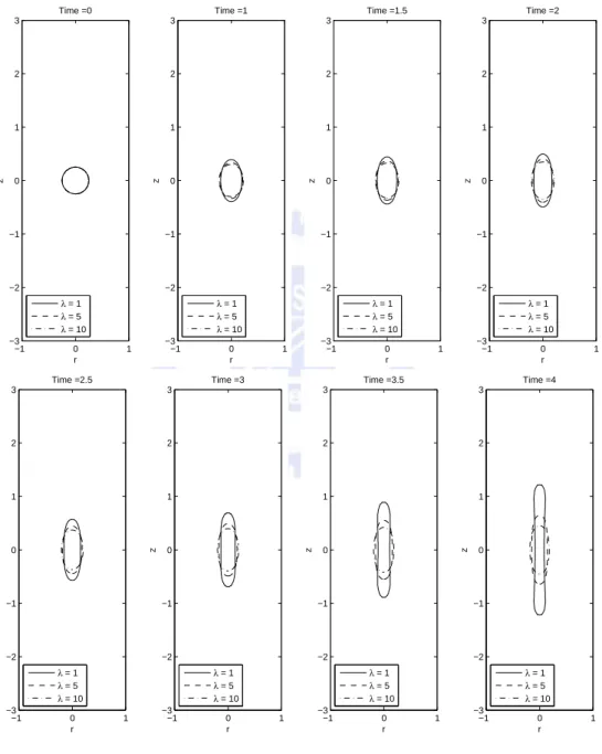
In general, a drop will be stretched along the direction of fluid flow if it is put into the extensional flow. But there is surface tension on the interface, it may restrict a tendency of stretching drop. Therefore,we first observe a property for the clean drop with the viscosity ratio λ = 1, 5 and 10, and we fix µ2 = 1 in this
computation. −1 0 1 −3 −2 −1 0 1 2 3 r z Time =0 λ = 1 λ = 5 λ = 10 −1 0 1 −3 −2 −1 0 1 2 3 r z Time =1 λ = 1 λ = 5 λ = 10 −1 0 1 −3 −2 −1 0 1 2 3 r z Time =1.5 λ = 1 λ = 5 λ = 10 −1 0 1 −3 −2 −1 0 1 2 3 r z Time =2 λ = 1 λ = 5 λ = 10 −1 0 1 −3 −2 −1 0 1 2 3 r z Time =2.5 λ = 1 λ = 5 λ = 10 −1 0 1 −3 −2 −1 0 1 2 3 r z Time =3 λ = 1 λ = 5 λ = 10 −1 0 1 −3 −2 −1 0 1 2 3 r z Time =3.5 λ = 1 λ = 5 λ = 10 −1 0 1 −3 −2 −1 0 1 2 3 r z Time =4 λ = 1 λ = 5 λ = 10
Figure 4.2: The time evolution of a drop in an extensional flow with λ = 1, 5 and 10 at T = 4.
Viscosity describes a fluid’s internal resistance to flow and may be thought of as a measure of fluid friction. For example, high-viscosity magma will create a tall, steep stratovolcano, because it cannot flow far before it cools, while low-viscosity lava will create a wide, shallow-sloped shield volcano. We can observe the defor-mation of the drop by flow in Fig.4.2, and as λ = 1, 5, and 10 the tip point of the interface on the z−axis are at about the positions (r, z) ≈ (0, ±1.221), (0, ±0.6437) and (0, ±0.4515),respectively at T = 4. By Eq.2.6 we know that E is the rate of deformation rate and the larger viscosity leads to smaller E. That is, the harde the drop will deform. We can observe this phenomenon from Fig.4.2. Thus drop is more sticky as viscosity is higher, the shape of drop is more difficult to be affected by flow. We then examine how the bubble would deform when viscosity of the inside drop is smaller than that of outside drop, i.e., viscosity ratio λ ≤ 1. We also observe effects of the clean drop deformation on the viscosity in an extensional flow , ur = −0.5Gr and uz = Gz, where G is the principal strain rate [6], and is chosen
as G = 1. Throughout this computation, the computational domain is chosen as Ω = [0, 1] × [−3, 3] in the axisymmetrical cylindrical coordinates, and the initial drop is chosen as a circular one with radius r0 = 0.25. We also fix the density
inside and outside the drop ρ1 = ρ2 = 1, the viscosity inside drop µ1 = 1, the
Reynolds number Re = 1, and the Capillary number Ca = 0.6. Here, we use the
mesh h = ∆x = ∆y = 1/64, the Lagrangian grid with size ∆s ≈ h, the time step size ∆t = h/8, and computed up to time T = 4.
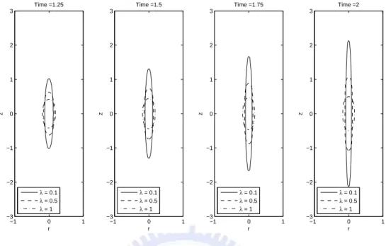
−1 0 1 −3 −2 −1 0 1 2 3 r z Time =0 λ = 1 λ = 5 λ = 10 −1 0 1 −3 −2 −1 0 1 2 3 r z Time =0.5 λ = 0.1 λ = 0.5 λ = 1 −1 0 1 −3 −2 −1 0 1 2 3 r z Time =0.75 λ = 0.1 λ = 0.5 λ = 1 −1 0 1 −3 −2 −1 0 1 2 3 r z Time =1 λ = 0.1 λ = 0.5 λ = 1
−1 0 1 −3 −2 −1 0 1 2 3 r z Time =1.25 λ = 0.1 λ = 0.5 λ = 1 −1 0 1 −3 −2 −1 0 1 2 3 r z Time =1.5 λ = 0.1 λ = 0.5 λ = 1 −1 0 1 −3 −2 −1 0 1 2 3 r z Time =1.75 λ = 0.1 λ = 0.5 λ = 1 −1 0 1 −3 −2 −1 0 1 2 3 r z Time =2 λ = 0.1 λ = 0.5 λ = 1
Figure 4.3: The time evolution of a drop in an extensional flow with λ = 0.1, 0.5 and 1 at T = 2.
We can observe the deformation of the drop by flow in Fig.4.3, and as λ = 0.1, 0.5, and 1 the tip point of the interface on the z−axis are at about the positions (r, z) ≈ (0, ±2.1323), (0, ±1.0702) and (0, ±0.4951),respectively at T = 2. As above we observe the deformation of drop is more intense when viscosity ration is lower. From Fig.4.2 and Fig.4.3, we notice the velocity of drop deformation with viscosity ratio λ < 1 is faster than that with viscosity ratio λ > 1. By Eq.2.6 we know that E is the rate of deformation rate and the larger viscosity leads to smaller E. As viscosity ratio λ < 1, we can think of it as viscosity outside drop µ2 < 1 and
viscosity inside drop µ1 = 1. Therefore we can perceive that the drop would be
easier to deform from Fig.4.3. Thus drop is less sticky as viscosity is higher, the shape of drop is easier to be affected by flow.
4.4
Effects of the drop deformation on surfactant
There is different behavior for clean interface and contaminated interface, so we will study it in this subsection. We compare a clean drop with a contaminated drop in an extensional flow, ur= −0.5Gr and uz = Gz, where G = 1. By the comparison,
we observe that the surface tension reduces when the surfactant is on the interface. Here, we use the mesh h = ∆x = ∆y = 1/64, the Lagrangian grid with size ∆s ≈ h, and the time step size ∆t = h/8.
The problem is set up as a drop immersed in a fluid domain Ω = [0, 1] × [−3, 3] with viscosity 1, which the drop is a circle with radius r0 = 0.25. We also fix the
den-sity inside and outside the drop ρ1 = ρ2 = 1, the Reynolds number Re = 1, the
Cap-illary number Ca = 0.6,and the surface Peclet number Pes = 1.25. The initial
surfac-tant concentration is uniformly distributed along the interface such as Γ (0, s) = 0.5, and the parameters in E.q.2.23 are chosen as σc= 1 and β = 0.5,respectively. We
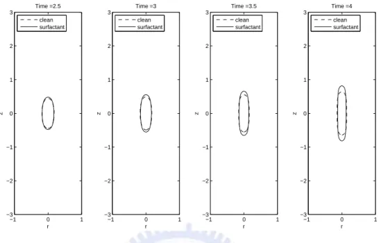
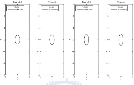
ex-amine viscosity ratio λ = 1, 5 and 10 repeatedly and observe the distinction between the clean interface (no surfactant) and contaminated interface (with surfactant).
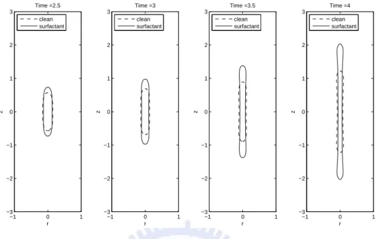
−1 0 1 −3 −2 −1 0 1 2 3 r z Time =0 clean surfactant −1 0 1 −3 −2 −1 0 1 2 3 r z Time =1 clean surfactant −1 0 1 −3 −2 −1 0 1 2 3 r z Time =1.5 clean surfactant −1 0 1 −3 −2 −1 0 1 2 3 r z Time =2 clean surfactant
−1 0 1 −3 −2 −1 0 1 2 3 r z Time =2.5 clean surfactant −1 0 1 −3 −2 −1 0 1 2 3 r z Time =3 clean surfactant −1 0 1 −3 −2 −1 0 1 2 3 r z Time =3.5 clean surfactant −1 0 1 −3 −2 −1 0 1 2 3 r z Time =4 clean surfactant
Figure 4.4: The time evolution of a drop in an extensional flow with λ = 1.
From the Fig4.4, the tip points of the interface on the z-axis are about at the positions (r, z) ≈ (0, ±2.0376), then we obtain the distance of contaminated drop from the tip point to the center is larger than that of clean drop. We observe the contaminated drop deforms more intensely because surfactant decrease the surface tension, causing the drop more likely to deform.
−1 0 1 −3 −2 −1 0 1 2 3 r z Time =0 clean surfactant −1 0 1 −3 −2 −1 0 1 2 3 r z Time =1 clean surfactant −1 0 1 −3 −2 −1 0 1 2 3 r z Time =1.5 clean surfactant −1 0 1 −3 −2 −1 0 1 2 3 r z Time =2 clean surfactant
−1 0 1 −3 −2 −1 0 1 2 3 r z Time =2.5 clean surfactant −1 0 1 −3 −2 −1 0 1 2 3 r z Time =3 clean surfactant −1 0 1 −3 −2 −1 0 1 2 3 r z Time =3.5 clean surfactant −1 0 1 −3 −2 −1 0 1 2 3 r z Time =4 clean surfactant
Figure 4.5: The time evolution of a drop in an extensional flow with λ = 5.
From the Fig4.5, the tip points of the interface on the z-axis are about at the positions (r, z) ≈ (0, ±0.8187), then we also obtain the distance of contaminated drop from the tip point to the center is larger than that of clean drop. Then, We examine viscosity ratio λ = 10 and observe the distinction between the clean interface (no surfactant) and contaminated interface (with surfactant).
−1 0 1 −3 −2 −1 0 1 2 3 r z Time =0 clean surfactant −1 0 1 −3 −2 −1 0 1 2 3 r z Time =1 clean surfactant −1 0 1 −3 −2 −1 0 1 2 3 r z Time =1.5 clean surfactant −1 0 1 −3 −2 −1 0 1 2 3 r z Time =2 clean surfactant
−1 0 1 −3 −2 −1 0 1 2 3 r z Time =2.5 clean surfactant −1 0 1 −3 −2 −1 0 1 2 3 r z Time =3 clean surfactant −1 0 1 −3 −2 −1 0 1 2 3 r z Time =3.5 clean surfactant −1 0 1 −3 −2 −1 0 1 2 3 r z Time =4 clean surfactant
Figure 4.6: The time evolution of a drop in an extensional flow with λ = 10.
From the Fig4.6, the tip points of the interface on the z-axis are about at the positions (r, z) ≈ (0, ±0.4929), then we we also obtain the distance of contaminated drop from the tip point to the center is larger than that of clean drop.
0 0.5 1 1.5 2 2.5 3 3.5 4 0.392 0.3921 0.3922 0.3923 0.3924 0.3925 0.3926 0.3927 0.3928 0.3929 0.393 Time Mass
Figure 4.7: This is the total mass of surfactant for P es = 1.25.
Even though surfactant would affect the drop deformation, viscosity is the main factor, and flow is more sticky as viscosity is higher, the shape of drop is more difficult to be affected by flow. Since the surfactant is insoluble, the total mass of the surfactant must be conserved In Fig.4.7, no matter which viscosity we choose, the total mass of surfactant for P es= 1.25 is conserved very well by our method.
4.5
Effects of the drop deformation on Peclet number
In this subsection, we compare the influence of different surface Peclet number
P eson the elongation of contaminated drop, and we choose peclet number P es from
0 to 500, partitioned 50 choices at once. Here, we first put a contaminated drop in the extensional flow, ur = −0.5Gr and uz = Gz, where G = 1 and compute up to
T = 4 in the domain Ω = [0, 1] × [−3, 3]. Then, we fix the Reynolds number Re= 1,
the Capillary number Ca = 0.3,and Γ (0, s) = 0.5 with the parameters in E.q.2.23 chosen as σc= 1 and β = 0.5,respectively.
Figure 4.8: Drop in axisymmetric flow.
A convenient method for expressing the results of experiment is to measure L, the length of the drop in the direction of the r axis, and B, the breadth in the direction of the z axis. As noting in Fig.4.8, the degree of deformation can be characterized by the scalar Df that was originally introduced by Taylor [11].
Df = L − B L + B (4.1) 0 50 100 150 200 250 300 350 400 450 500 0.2 0.22 0.24 0.26 0.28 0.3 0.32 0.34 0.36 0.38 0.4 Peclet number Pes degree of deformation Df
0 0.5 1 1.5 2 2.5 3 3.5 4 0.628 0.6281 0.6282 0.6283 0.6284 0.6285 0.6286 0.6287 0.6288 0.6289 0.629 Time Mass
Figure 4.10: This is the total mass of surfactant for every Peclet number P es.
Since the underlying extensional drives the surfactant toward to the tip points of the drop, the surfactant concentration is higher and thus the surface tension is lower near the tips. When the Peclet number is lager, the surfactant gradient along the interface is lager too, therefore, the overall drop elongation is greater. From Fig.4.9 we noticed from Peclet number P es from 0 to 150 the larger the deformation the
more obvious, but past 150 the larger the change will also be additional, but the higher the number the higher the tendency to plateau. By Fig.4.10 we also obtain the total mass of surfactant conserved no matter Peclet number which we choose.
5
Conclusion
In this paper, we used the immersed boundary method such that the interface is in the different phases with different densities and viscosities by an indicator function in the cylindrical coordinates to construct our formulation. Since the velocity field is in the axisymmetric coordinates, the velocity boundary conditions on r = 0 must be set ur = 0 and ∂uz/∂r = 0.We solve the Navier-Stokes equations by projection
method, and update the new marker positions by imposing the artificial velocity in order to make the new positions uniformly. Controlling marker positions uni-formly can make the volume error smaller. Similarly, the surfactant equation must impose the artificial velocities to control the concentration locations. The surface tension is reduced by the surfactant, and Peclet number influences the diffusion of the surfactant.
In our future work, for a drop on a solid, controlling the equilibrium contact angle can produce the hydrophobic phenomenon or hydrophilic phenomenon. Imposing the surfactant on the interface affects the equilibrium contact angle in this mov-ing contact line case. Furthermore, we can develop the more general 3-dimension simulation.
References
[1] David L. Brown, Ricardo Cortez, and Michael L. Minion, “Accurate projection methods for the incompressible NavierVStokes equations.” Journal of
Compu-tational Physics, Vol. 168, (2001), pp. 464-499.
[2] Charles D. Eggleton, Tse-Min Tsai, and Kathleen J. Stebe, “Tip streaming from a drop in the presence of surfactants.” Physical Review Letters, Vol. 87, No. 4, (2001), pp. from 048302-1 to 048302-4.
[3] Wei-Xi Huang, Soo Jai Shin, and Hyung Jin Sung, “Simulation of flexible filaments in a uniform flow by the immersed boundary method.” Journal of
Computational Physics, Vol. 226, (2007), pp. 2206-2228.
[4] Ming-Chih Lai, Wen-Wei Lin, and Weichung Wang, “A fast spectral/differnce method without pole conditions for Poisson-type equations in cylindrical and spherical geometries.” IMA Journal of Numerical Analysis, Vol. 22, (2002), pp. 537-548.
[5] Ming-Chih Lai, Yu-Hau Tseng, and Huaxiong Huang, “An immersed boundary method for interfacial flows with insoluble surfactant.” Journal of
Computa-tional Physics, Vol. 227, (2008), pp. 7279-7293.
[6] Jie Li, “The effect of an insoluble surfactant on the skin friction of a bubble.”
European Journal of Mechanics B/Fluid, 25 (2006) 59-73
[7] J. M. Lopez and Jie Shen, “An efficient spectral-projection method for the Navier-Stokes equations in cylindrical geometies, I. Axisymmetric cases.”
Jour-nal of ComputatioJour-nal Physics, Vol. 139, (1998), pp. 308-326.
[8] Charles S. Peskin and Beth Feller Printz, “Improved volume conservation in the computation of flows with immersed elastic boundaries.” Journal of
Com-putational Physics, Vol. 105, (1993), pp. 33-46.
[9] H.A. Stone, “A simple derivation of the time-dependent convective-diffusion equation for surfactant transport along adeforming interface.” Phys. Fluids A 2 (1), (1990), pp. 111-112.
[10] H. A. Stone and L. G. Leal, “The effects of surfactants on drop deformation and breakup.” J. Fluid Mech., Vol. 220, (1990), pp. 161-186.
[11] G.I. Taylor, The formation of emulsions in definable fields of flow, Proc. R. Soc. Lond. A 146 (1934) 501.
[12] G. Tryggvason, B. Bunner, A. Esmaeeli, D. Juric, N. Al-Rawahi, W. Tauber, J. Han, S. Nas, Y.-J. Jan, A front-tracking method for the computations of multiphase flow, J. Comput. Phys., 169 (2001) 708-759
[13] Salih Ozen Unverdi and Gr´etar Tryggvason, “A Front-Tracking Method for Viscous, Incompressible, Multi-fluid Flows.” Journal of computational physics, 100, pp. 25-37 (1992)
[14] Etienne Guyon, Jean-Pierre Hulin, Luc Petit, and Catalin D. Mitescu,“Physical hydrodynamics.” Oxford University Press, USA, (2001)