應用於高密度光儲存系統讀取信號之模擬

(1)

國

立

交

通

大

學

光電工程研究所

碩士論文

應用於高密度光儲存系統讀取信號之模擬

Optical Readout Waveforms Simulation in

High Density Optical Storage System

研究生: 高維樑

指導教授: 田仲豪博士

中華民國九十五年七月

(2)

應用於高密度光儲存系統讀取信號之模擬

Optical Readout Waveforms Simulation in

High Density Optical Storage System

研究生: 高維樑 Student: Wei‐Liang Kao

指導教授: 田仲豪 Advisor: Dr. Chung‐Hao Tien

國立交通大學電機學院

光電工程研究所

碩士論文

A Thesis

Submitted to Institute of Electro‐Optical Engineering

College of Electrical Engineering and Computer Science

National Chiao‐Tung University

in Partial Fulfillment of the Requirements

for the Degree of

Master

In

Electro‐Optical Engineering

June 2006

Hsin‐Chu, Taiwan, Republic of China

中華民國九十五年七月

(3)

應用於高密度光儲存系統讀取信號之模擬

研究生: 高維樑

指導教授: 田仲豪博士

國立交通大學光電工程研究所

摘要

隨著對於儲存容量需求的增加，光儲存系統採用較短的波長以及較高的數值孔徑的物鏡，來達成此一目的。但當較高數值孔徑的物鏡被採用時，光的向量繞射特性就應該納入考量。因此，本論文提出了一個結合了「光追跡」與「向量繞射」優點的光學讀取頭模型，不但可以節省計算時間，亦可以達到相當的準確度。基於先前所提出的光學讀取頭模型，並以DVD+R/RW為例，成功地模擬出其讀取信號(RF signal)、聚焦伺服信號(FES)以及尋軌伺服信號(TES)，並與規格書的標準做比較，以驗證模擬結果的可靠度。此外，本論文也對DVD+R/RW系統，進行公差分析(Tolerance analysis)，其中包含傾斜(Tilt)公差與失焦(Defocus) 公差，並與實驗結果作比較，討論公差對於讀出信號及伺服信號的影響。最後，本論文討論了一種在可寫入及可覆寫式系統中常見的現象－饋通現象 (Feedthrough)。此現象主要是發生在碟機尋軌時，由於碟片上的溝軌結構 (Groove structure)使得聚焦伺服信號會隨著尋軌伺服信號變動的一種干擾 (Crosstalk)。此現象會影響聚焦伺服的穩定度，在本論文中會討論其成因以及影響其變化的因素。可以藉由本論文所提出的光學讀取頭模型的模擬分析，用來在先前設計的步驟當中，發現可能的問題，以期能在發現問題的初步，就能夠找出可能原因，進一步提出解決方案。亦可用於當在碟機系統中發現問題時，將其與以往的模擬結果作比對，以反向推導的方式找出問題可能的原因。

(4)

Optical Readout Waveforms Simulation in

High Density Optical Storage System

Student: Wei‐Liang Kao Advisor: Chung‐Hao Tien

Institute of Electro‐Optical Engineering

National Chiao Tung University

Abstract

As the coming of the tera‐era, the demand for the storage capacity is increasing. It is known that the storage capacity is governed by the ratio of wavelength (λ) of the laser diode and the numerical aperture (NA) of the objective lens. Therefore, the optical data storage system is developed toward a shorter wavelength and a higher NA. When the NA of the objective lens is higher than 0.6, the vector nature of light will play an important role during readout process. The optical model combined the advantages of the ray‐tracing and vector diffraction is proposed to achieve a faster calculation and still maintain the reliability.

Based on the proposed model, the RF signal and servo signals including the focus error signal (FES) and tracking error signals (TES) are demonstrated and successfully verified with the specification under DVD+R/RW system. Moreover, the tolerance analysis of DVD+R/RW system is accomplished. The tilt and defocus effect are simulated and compared with the experimental results to show how the tolerance affect the readout and

(5)

servo signals. Finally, this thesis discusses a phenomenon which will happen especially in the recordable and re‐writable systems called feedthrough. The feedthrough effect is caused by the groove structures on the recordable disc and lead to a variation in focus error signal with the tracking error signal during track seeking process. The feedthrough effect will deteriorated the performance of the focus servo and the origin and the factors that influence feedthrough are discussed.

(6)

Acknowledgement

During my graduate life, I am especially grateful to Professor Chung‐Hao Tien, who gave me many valuable advises in research and English presentation skills. Professor Tien provides an excellent environment for me and let me finish my graduate diploma smoothly.

My classmates, Yen‐Hsing Lu, Che‐Jen Lin, Ming‐Jing Chien, Chien‐Hsiang Hung and Pi‐Ju Cheng, have accompanied me for these two years and made my graduate life colorful and full of joy. The junior classmates, Shih‐Wei Ying, Yuan‐Jung Yao, Tzu‐Hsiang Lan, Shun‐Ting Hsiao, and Cho‐Chih Chen, also help me a lot in study and bring me a nice memory in my last graduate year. Besides, special thanks to the other classmates in Rm.601 form the warm and happy ambiance for me as well. Moreover, Paul, the French international student, gives me a fresh and nice experience about France. I also want to show my appreciation to Yen‐Chih Lee and Wen‐Chun Feng, who help me a lot in experiment and give me many useful suggestions about my thesis. Finally, but essentially, I owe to my parents, grandparents, aunts and my family successful completion of my study. They support me with all their heart to let me complete my study without the fear of disturbance in the rear. Without my family, I could not be what I am today.

Wei‐Liang Vic Kao July, 2006

(7)

Abstract (Chinese) ‐‐‐‐‐‐‐‐‐‐‐‐‐‐‐‐‐‐‐‐‐‐‐‐‐‐‐‐‐‐‐‐‐‐‐‐‐‐‐‐‐‐‐‐‐‐‐‐‐‐‐‐‐‐‐‐‐‐‐‐‐‐‐‐‐‐‐‐‐‐‐‐‐‐‐‐‐‐‐‐ i Abstract (English) ‐‐‐‐‐‐‐‐‐‐‐‐‐‐‐‐‐‐‐‐‐‐‐‐‐‐‐‐‐‐‐‐‐‐‐‐‐‐‐‐‐‐‐‐‐‐‐‐‐‐‐‐‐‐‐‐‐‐‐‐‐‐‐‐‐‐‐‐‐‐‐‐‐‐‐‐‐‐‐ ii Acknowledgement ‐‐‐‐‐‐‐‐‐‐‐‐‐‐‐‐‐‐‐‐‐‐‐‐‐‐‐‐‐‐‐‐‐‐‐‐‐‐‐‐‐‐‐‐‐‐‐‐‐‐‐‐‐‐‐‐‐‐‐‐‐‐‐‐‐‐‐‐‐‐‐‐‐‐‐‐‐‐iv Table of Contents ‐‐‐‐‐‐‐‐‐‐‐‐‐‐‐‐‐‐‐‐‐‐‐‐‐‐‐‐‐‐‐‐‐‐‐‐‐‐‐‐‐‐‐‐‐‐‐‐‐‐‐‐‐‐‐‐‐‐‐‐‐‐‐‐‐‐‐‐‐‐‐‐‐‐‐‐‐‐‐‐ v Figure Captions ‐‐‐‐‐‐‐‐‐‐‐‐‐‐‐‐‐‐‐‐‐‐‐‐‐‐‐‐‐‐‐‐‐‐‐‐‐‐‐‐‐‐‐‐‐‐‐‐‐‐‐‐‐‐‐‐‐‐‐‐‐‐‐‐‐‐‐‐‐‐‐‐‐‐‐‐‐‐‐‐‐ vii List of Tables ‐‐‐‐‐‐‐‐‐‐‐‐‐‐‐‐‐‐‐‐‐‐‐‐‐‐‐‐‐‐‐‐‐‐‐‐‐‐‐‐‐‐‐‐‐‐‐‐‐‐‐‐‐‐‐‐‐‐‐‐‐‐‐‐‐‐‐‐‐‐‐‐‐‐‐‐‐‐‐‐‐‐‐‐ xii

Chapter 1 Introduction ‐‐‐‐‐‐‐‐‐‐‐‐‐‐‐‐‐‐‐‐‐‐‐‐‐‐‐‐‐‐‐‐‐‐‐‐‐‐‐‐‐‐‐‐‐‐‐‐‐‐‐‐‐‐‐‐‐‐ 1

1.1 Motivation‐‐‐‐‐‐‐‐‐‐‐‐‐‐‐‐‐‐‐‐‐‐‐‐‐‐‐‐‐‐‐‐‐‐‐‐‐‐‐‐‐‐‐‐‐‐‐‐‐‐‐‐‐‐‐‐‐‐‐‐‐‐‐‐‐‐‐‐‐‐‐‐‐‐‐‐‐‐‐‐‐‐‐‐‐‐ 1 1.2 Objectives ‐‐‐‐‐‐‐‐‐‐‐‐‐‐‐‐‐‐‐‐‐‐‐‐‐‐‐‐‐‐‐‐‐‐‐‐‐‐‐‐‐‐‐‐‐‐‐‐‐‐‐‐‐‐‐‐‐‐‐‐‐‐‐‐‐‐‐‐‐‐‐‐‐‐‐‐‐‐‐‐‐‐‐‐‐‐ 4 1.3 Organization ‐‐‐‐‐‐‐‐‐‐‐‐‐‐‐‐‐‐‐‐‐‐‐‐‐‐‐‐‐‐‐‐‐‐‐‐‐‐‐‐‐‐‐‐‐‐‐‐‐‐‐‐‐‐‐‐‐‐‐‐‐‐‐‐‐‐‐‐‐‐‐‐‐‐‐‐‐‐‐‐‐‐‐ 5

Chapter 2 Principles and Literature Review ‐‐‐‐‐‐‐‐‐‐‐‐‐‐‐‐‐‐‐‐‐‐‐‐‐‐‐‐‐‐ 6

2.1 Scalar and Vector Diffraction Theory ‐‐‐‐‐‐‐‐‐‐‐‐‐‐‐‐‐‐‐‐‐‐‐‐‐‐‐‐‐‐‐‐‐‐‐‐‐‐‐‐‐‐‐‐‐‐‐‐‐‐‐ 6 2.1.1 Scalar Diffraction Theory ‐‐‐‐‐‐‐‐‐‐‐‐‐‐‐‐‐‐‐‐‐‐‐‐‐‐‐‐‐‐‐‐‐‐‐‐‐‐‐‐‐‐‐‐‐‐‐‐‐‐‐‐‐‐‐‐‐‐‐‐‐ 7 2.1.2 Vector Diffraction Theory ‐‐‐‐‐‐‐‐‐‐‐‐‐‐‐‐‐‐‐‐‐‐‐‐‐‐‐‐‐‐‐‐‐‐‐‐‐‐‐‐‐‐‐‐‐‐‐‐‐‐‐‐‐‐‐‐‐‐‐ 12 2.1.3 Comparison ‐‐‐‐‐‐‐‐‐‐‐‐‐‐‐‐‐‐‐‐‐‐‐‐‐‐‐‐‐‐‐‐‐‐‐‐‐‐‐‐‐‐‐‐‐‐‐‐‐‐‐‐‐‐‐‐‐‐‐‐‐‐‐‐‐‐‐‐‐‐‐‐‐‐‐‐‐ 15 2.2 The Babinet Principle ‐‐‐‐‐‐‐‐‐‐‐‐‐‐‐‐‐‐‐‐‐‐‐‐‐‐‐‐‐‐‐‐‐‐‐‐‐‐‐‐‐‐‐‐‐‐‐‐‐‐‐‐‐‐‐‐‐‐‐‐‐‐‐‐‐‐‐‐‐‐ 19 2.2.1 Mathematical Formulation and Physical Description ‐‐‐‐‐‐‐‐‐‐‐‐‐‐‐‐‐‐‐‐‐‐‐‐ 19 2.2.2 Generating the Readout, Servo, and Cross‐talk ‐‐‐‐‐‐‐‐‐‐‐‐‐‐‐‐‐‐‐‐‐‐‐‐‐‐‐‐‐‐‐‐ 22 2.2.3 Applications of the Babinet principle ‐‐‐‐‐‐‐‐‐‐‐‐‐‐‐‐‐‐‐‐‐‐‐‐‐‐‐‐‐‐‐‐‐‐‐‐‐‐‐‐‐‐‐‐‐ 25 2.2.4 Summary ‐‐‐‐‐‐‐‐‐‐‐‐‐‐‐‐‐‐‐‐‐‐‐‐‐‐‐‐‐‐‐‐‐‐‐‐‐‐‐‐‐‐‐‐‐‐‐‐‐‐‐‐‐‐‐‐‐‐‐‐‐‐‐‐‐‐‐‐‐‐‐‐‐‐‐‐‐‐‐‐ 27 2.3 Servo mechanisms ‐‐‐‐‐‐‐‐‐‐‐‐‐‐‐‐‐‐‐‐‐‐‐‐‐‐‐‐‐‐‐‐‐‐‐‐‐‐‐‐‐‐‐‐‐‐‐‐‐‐‐‐‐‐‐‐‐‐‐‐‐‐‐‐‐‐‐‐‐‐‐‐‐‐ 28 2.3.1 Focus Servo ‐‐‐‐‐‐‐‐‐‐‐‐‐‐‐‐‐‐‐‐‐‐‐‐‐‐‐‐‐‐‐‐‐‐‐‐‐‐‐‐‐‐‐‐‐‐‐‐‐‐‐‐‐‐‐‐‐‐‐‐‐‐‐‐‐‐‐‐‐‐‐‐‐‐‐‐‐ 29 2.3.2 Tracking Servo ‐‐‐‐‐‐‐‐‐‐‐‐‐‐‐‐‐‐‐‐‐‐‐‐‐‐‐‐‐‐‐‐‐‐‐‐‐‐‐‐‐‐‐‐‐‐‐‐‐‐‐‐‐‐‐‐‐‐‐‐‐‐‐‐‐‐‐‐‐‐‐‐‐ 30 2.3.3 Servo Implementation Challenges ‐‐‐‐‐‐‐‐‐‐‐‐‐‐‐‐‐‐‐‐‐‐‐‐‐‐‐‐‐‐‐‐‐‐‐‐‐‐‐‐‐‐‐‐‐‐‐‐ 32 2.4 Summary ‐‐‐‐‐‐‐‐‐‐‐‐‐‐‐‐‐‐‐‐‐‐‐‐‐‐‐‐‐‐‐‐‐‐‐‐‐‐‐‐‐‐‐‐‐‐‐‐‐‐‐‐‐‐‐‐‐‐‐‐‐‐‐‐‐‐‐‐‐‐‐‐‐‐‐‐‐‐‐‐‐‐‐‐‐‐ 34

Chapter 3 Simulation Model ‐‐‐‐‐‐‐‐‐‐‐‐‐‐‐‐‐‐‐‐‐‐‐‐‐‐‐‐‐‐‐‐‐‐‐‐‐‐‐‐‐‐‐‐‐‐‐‐‐ 35

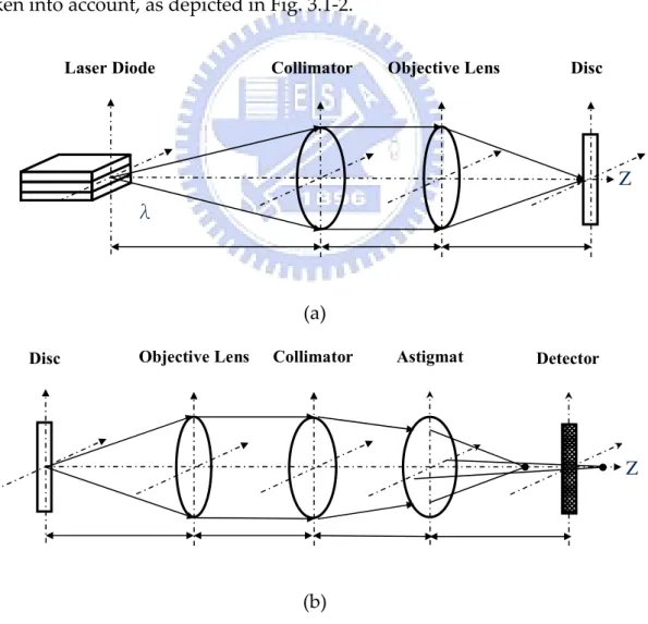
3.1 Simulation Description ‐‐‐‐‐‐‐‐‐‐‐‐‐‐‐‐‐‐‐‐‐‐‐‐‐‐‐‐‐‐‐‐‐‐‐‐‐‐‐‐‐‐‐‐‐‐‐‐‐‐‐‐‐‐‐‐‐‐‐‐‐‐‐‐‐‐‐‐ 35 3.1.1 Readout Model ‐‐‐‐‐‐‐‐‐‐‐‐‐‐‐‐‐‐‐‐‐‐‐‐‐‐‐‐‐‐‐‐‐‐‐‐‐‐‐‐‐‐‐‐‐‐‐‐‐‐‐‐‐‐‐‐‐‐‐‐‐‐‐‐‐‐‐‐‐‐‐‐‐ 38 3.1.2 Parameters ‐‐‐‐‐‐‐‐‐‐‐‐‐‐‐‐‐‐‐‐‐‐‐‐‐‐‐‐‐‐‐‐‐‐‐‐‐‐‐‐‐‐‐‐‐‐‐‐‐‐‐‐‐‐‐‐‐‐‐‐‐‐‐‐‐‐‐‐‐‐‐‐‐‐‐‐‐‐ 39 3.1.3 Simulation Tool ‐‐‐‐‐‐‐‐‐‐‐‐‐‐‐‐‐‐‐‐‐‐‐‐‐‐‐‐‐‐‐‐‐‐‐‐‐‐‐‐‐‐‐‐‐‐‐‐‐‐‐‐‐‐‐‐‐‐‐‐‐‐‐‐‐‐‐‐‐‐‐‐ 40 3.2 System Construction ‐‐‐‐‐‐‐‐‐‐‐‐‐‐‐‐‐‐‐‐‐‐‐‐‐‐‐‐‐‐‐‐‐‐‐‐‐‐‐‐‐‐‐‐‐‐‐‐‐‐‐‐‐‐‐‐‐‐‐‐‐‐‐‐‐‐‐‐‐‐‐ 41

(8)

3.3 Tolerance Issues ‐‐‐‐‐‐‐‐‐‐‐‐‐‐‐‐‐‐‐‐‐‐‐‐‐‐‐‐‐‐‐‐‐‐‐‐‐‐‐‐‐‐‐‐‐‐‐‐‐‐‐‐‐‐‐‐‐‐‐‐‐‐‐‐‐‐‐‐‐‐‐‐‐‐‐‐‐ 45 3.3.1 Tilt Effects ‐‐‐‐‐‐‐‐‐‐‐‐‐‐‐‐‐‐‐‐‐‐‐‐‐‐‐‐‐‐‐‐‐‐‐‐‐‐‐‐‐‐‐‐‐‐‐‐‐‐‐‐‐‐‐‐‐‐‐‐‐‐‐‐‐‐‐‐‐‐‐‐‐‐‐‐‐‐‐ 45 3.3.2 Defocus Effects ‐‐‐‐‐‐‐‐‐‐‐‐‐‐‐‐‐‐‐‐‐‐‐‐‐‐‐‐‐‐‐‐‐‐‐‐‐‐‐‐‐‐‐‐‐‐‐‐‐‐‐‐‐‐‐‐‐‐‐‐‐‐‐‐‐‐‐‐‐‐‐‐‐ 47 3.4 Jitter Analysis ‐‐‐‐‐‐‐‐‐‐‐‐‐‐‐‐‐‐‐‐‐‐‐‐‐‐‐‐‐‐‐‐‐‐‐‐‐‐‐‐‐‐‐‐‐‐‐‐‐‐‐‐‐‐‐‐‐‐‐‐‐‐‐‐‐‐‐‐‐‐‐‐‐‐‐‐‐‐‐‐ 49 3.5 Summary ‐‐‐‐‐‐‐‐‐‐‐‐‐‐‐‐‐‐‐‐‐‐‐‐‐‐‐‐‐‐‐‐‐‐‐‐‐‐‐‐‐‐‐‐‐‐‐‐‐‐‐‐‐‐‐‐‐‐‐‐‐‐‐‐‐‐‐‐‐‐‐‐‐‐‐‐‐‐‐‐‐‐‐‐‐‐ 51

Chapter 4 Simulation Results ‐‐‐‐‐‐‐‐‐‐‐‐‐‐‐‐‐‐‐‐‐‐‐‐‐‐‐‐‐‐‐‐‐‐‐‐‐‐‐‐‐‐‐‐‐‐‐ 52

4.1 Results 1 – Readout Waveforms ‐‐‐‐‐‐‐‐‐‐‐‐‐‐‐‐‐‐‐‐‐‐‐‐‐‐‐‐‐‐‐‐‐‐‐‐‐‐‐‐‐‐‐‐‐‐‐‐‐‐‐‐‐‐‐‐ 52 4.2 Results 2 – Servo Signals: FES & TES ‐‐‐‐‐‐‐‐‐‐‐‐‐‐‐‐‐‐‐‐‐‐‐‐‐‐‐‐‐‐‐‐‐‐‐‐‐‐‐‐‐‐‐‐‐‐‐‐‐‐ 58 4.3 Results 3 – Tolerance Analysis ‐‐‐‐‐‐‐‐‐‐‐‐‐‐‐‐‐‐‐‐‐‐‐‐‐‐‐‐‐‐‐‐‐‐‐‐‐‐‐‐‐‐‐‐‐‐‐‐‐‐‐‐‐‐‐‐‐‐ 64 4.2.1 Tilt ‐‐‐‐‐‐‐‐‐‐‐‐‐‐‐‐‐‐‐‐‐‐‐‐‐‐‐‐‐‐‐‐‐‐‐‐‐‐‐‐‐‐‐‐‐‐‐‐‐‐‐‐‐‐‐‐‐‐‐‐‐‐‐‐‐‐‐‐‐‐‐‐‐‐‐‐‐‐‐‐‐‐‐‐‐‐‐‐‐ 64 4.2.2 Defocus ‐‐‐‐‐‐‐‐‐‐‐‐‐‐‐‐‐‐‐‐‐‐‐‐‐‐‐‐‐‐‐‐‐‐‐‐‐‐‐‐‐‐‐‐‐‐‐‐‐‐‐‐‐‐‐‐‐‐‐‐‐‐‐‐‐‐‐‐‐‐‐‐‐‐‐‐‐‐‐‐‐‐‐ 68 4.3 Results 4 – Feedthrough: the crosstalk between TES & FES ‐‐‐‐‐‐‐‐‐‐‐‐‐‐‐‐‐‐‐‐‐‐ 71 4.4 Summary ‐‐‐‐‐‐‐‐‐‐‐‐‐‐‐‐‐‐‐‐‐‐‐‐‐‐‐‐‐‐‐‐‐‐‐‐‐‐‐‐‐‐‐‐‐‐‐‐‐‐‐‐‐‐‐‐‐‐‐‐‐‐‐‐‐‐‐‐‐‐‐‐‐‐‐‐‐‐‐‐‐‐‐‐‐‐ 79

Chapter 5 Conclusion and Future Works ‐‐‐‐‐‐‐‐‐‐‐‐‐‐‐‐‐‐‐‐‐‐‐‐‐‐‐‐‐‐‐‐‐ 80

6.1 Conclusion ‐‐‐‐‐‐‐‐‐‐‐‐‐‐‐‐‐‐‐‐‐‐‐‐‐‐‐‐‐‐‐‐‐‐‐‐‐‐‐‐‐‐‐‐‐‐‐‐‐‐‐‐‐‐‐‐‐‐‐‐‐‐‐‐‐‐‐‐‐‐‐‐‐‐‐‐‐‐‐‐‐‐‐‐ 80 6.2 Future Works ‐‐‐‐‐‐‐‐‐‐‐‐‐‐‐‐‐‐‐‐‐‐‐‐‐‐‐‐‐‐‐‐‐‐‐‐‐‐‐‐‐‐‐‐‐‐‐‐‐‐‐‐‐‐‐‐‐‐‐‐‐‐‐‐‐‐‐‐‐‐‐‐‐‐‐‐‐‐‐‐ 82

Reference ‐‐‐‐‐‐‐‐‐‐‐‐‐‐‐‐‐‐‐‐‐‐‐‐‐‐‐‐‐‐‐‐‐‐‐‐‐‐‐‐‐‐‐‐‐‐‐‐‐‐‐‐‐‐‐‐‐‐‐‐‐‐‐‐‐‐‐‐‐‐‐‐‐‐ 84

(9)

Figure Captions

Chapter 1 Introduction

1.1 Motivation Fig. 1.1‐1 A diagram of the light paths for the CD, DVD and DVR system and electron microscope photographs of the information pits of the three systems ‐‐‐‐‐‐‐‐‐‐‐‐‐‐‐‐‐‐‐‐‐‐‐‐‐‐‐‐‐‐‐‐‐‐‐‐‐‐‐‐‐‐‐‐‐‐‐‐‐‐‐‐‐‐‐‐‐‐‐‐‐‐‐‐‐‐‐‐‐‐‐‐‐‐‐‐‐‐‐‐ 1

Chapter 2 Principles and Literature Review

2.1 Scalar and Vector Diffraction Theory Fig. 2.1‐1 Diffraction geometry ‐‐‐‐‐‐‐‐‐‐‐‐‐‐‐‐‐‐‐‐‐‐‐‐‐‐‐‐‐‐‐‐‐‐‐‐‐‐‐‐‐‐‐‐‐‐‐‐‐‐‐‐‐‐‐‐‐‐‐‐‐‐‐ 7 Fig. 2.1‐2 A linearly polarized beam is brought to focus by a lens ‐‐‐‐‐‐‐‐‐‐‐‐‐‐‐‐‐‐ 13 Fig. 2.1‐3 An x‐polarized Gaussian beam is focused by a lens with NA=0.45, and observe the intensity distribution of X‐, Y‐, and Z‐polarization (from the left to the right) on the focal plane. The calculation method is (a) vector diffraction theory, and (b) scalar diffraction theory ‐‐‐‐‐‐‐‐‐‐‐‐‐‐‐‐‐‐‐‐‐‐‐‐‐‐‐‐‐‐‐‐‐‐‐‐‐‐‐‐‐‐‐‐‐‐‐‐‐‐‐‐‐‐‐‐‐‐‐‐‐‐‐‐‐‐‐‐‐‐‐‐‐‐‐‐‐‐‐‐‐‐‐‐‐‐‐‐‐‐ 16 Fig. 2.1‐4 An x‐polarized Gaussian beam is focused by a lens with NA=0.85, and observe the intensity distribution of X‐, Y‐, and Z‐polarization (from the left to the right) on the focal plane. The calculation method is (a) vector diffraction theory, and (b) scalar diffraction theory. --- 17 2.2 The Babinet Principle Fig. 2.2‐1 Light is focused on the disc and formed a reflected field . The reflected field diffracts to form a field at the pupil of the ( , ) T U x y ~ ( ', ') T U x y objective lens ‐‐‐‐‐‐‐‐‐‐‐‐‐‐‐‐‐‐‐‐‐‐‐‐‐‐‐‐‐‐‐‐‐‐‐‐‐‐‐‐‐‐‐‐‐‐‐‐‐‐‐‐‐‐‐‐‐‐‐‐‐‐‐‐‐‐‐‐‐‐‐‐ 19 Fig. 2.2‐2 Track layout of the disc ‐‐‐‐‐‐‐‐‐‐‐‐‐‐‐‐‐‐‐‐‐‐‐‐‐‐‐‐‐‐‐‐‐‐‐‐‐‐‐‐‐‐‐‐‐‐‐‐‐‐‐‐‐‐‐‐‐‐‐ 21

(10)

Fig. 2.2‐3 The Babinet principle used to decompose the signal reflected by the optical disc ‐‐‐‐‐‐‐‐‐‐‐‐‐‐‐‐‐‐‐‐‐‐‐‐‐‐‐‐‐‐‐‐‐‐‐‐‐‐‐‐‐‐‐‐‐‐‐‐‐‐‐‐‐‐‐‐‐‐‐‐‐‐‐‐‐‐‐‐‐‐‐‐‐‐ 22 Fig. 2.2‐4 Different combinations of the reflection terms generate the servo signal, and two types of crosstalk ‐‐‐‐‐‐‐‐‐‐‐‐‐‐‐‐‐‐‐‐‐‐‐‐‐‐‐‐‐‐‐‐‐‐‐‐‐‐‐‐‐‐‐‐‐‐‐‐‐‐‐‐‐‐‐ 23 2.3 Servo mechanisms Fig. 2.3‐1 Schematic diagram of pick‐up head with focus servo and tracking servo ‐‐‐‐‐‐‐‐‐‐‐‐‐‐‐‐‐‐‐‐‐‐‐‐‐‐‐‐‐‐‐‐‐‐‐‐‐‐‐‐‐‐‐‐‐‐‐‐‐‐‐‐‐‐‐‐‐‐‐‐‐‐‐‐‐‐‐‐‐‐‐‐‐‐‐‐‐‐‐‐‐‐‐‐‐‐‐‐‐‐ 28

Fig. 2.3-2 Astigmatism focus error method --- 29

Fig. 2.3‐3 The push‐pull tracking method ‐‐‐‐‐‐‐‐‐‐‐‐‐‐‐‐‐‐‐‐‐‐‐‐‐‐‐‐‐‐‐‐‐‐‐‐‐‐‐‐‐‐‐‐‐‐‐‐‐ 31

Chapter 3 Simulation Model

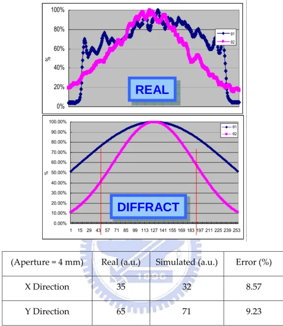
3.1 Simulation Description Fig. 3.1‐1 The configuration of the simulated DVD system ‐‐‐‐‐‐‐‐‐‐‐‐‐‐‐‐‐‐‐‐‐‐‐‐‐‐‐ 36 Fig. 3.1‐2 The unfolded optical path of the simulation model ‐‐‐‐‐‐‐‐‐‐‐‐‐‐‐‐‐‐‐‐‐‐‐ 37 (a) The incident optical path (b) the reflected optical path. Fig. 3.1‐3 Schematic diagram of the superposition of the sequential marks ‐‐‐‐‐ 38 3.2 System Construction Fig. 3.2‐1 Transformation from distance to angle ‐‐‐‐‐‐‐‐‐‐‐‐‐‐‐‐‐‐‐‐‐‐‐‐‐‐‐‐‐‐‐‐‐‐‐‐‐‐‐ 41 Fig. 3.2‐2 The comparison of simulated results and the specifications of the laser diode ‐‐‐‐‐‐‐‐‐‐‐‐‐‐‐‐‐‐‐‐‐‐‐‐‐‐‐‐‐‐‐‐‐‐‐‐‐‐‐‐‐‐‐‐‐‐‐‐‐‐‐‐‐‐‐‐‐‐‐‐‐‐‐‐‐‐‐‐‐‐‐‐‐‐‐‐‐‐‐‐‐‐ 42

Fig. 3.2-3 The comparisons of the rim intensities between the simulation and the real case

--- 43

(11)

3.3 Tolerance Issues Fig. 3.3‐1 The focused spot with coma aberration of ‐1λ ‐‐‐‐‐‐‐‐‐‐‐‐‐‐‐‐‐‐‐‐‐‐‐‐‐‐‐‐‐‐ 45 Fig. 3.3‐2 The focused spot with (a) spherical, and (b) defocus aberration ‐‐‐‐‐‐‐‐‐‐‐‐‐‐‐‐‐‐‐‐‐‐‐‐‐‐‐‐‐‐‐‐‐‐‐‐‐‐‐‐‐‐‐‐‐‐‐‐‐‐‐‐‐‐‐‐‐‐‐‐‐‐‐‐‐‐‐‐‐‐‐‐‐‐‐‐‐‐‐‐‐‐‐‐‐‐‐‐‐‐‐ 47 Fig. 3.3‐3 The relationship between the FES and the plot of Jitter vs. Defocus ‐‐ 48 3.4 Jitter Analysis Fig. 3.4‐1 Time interval analysis and the definition of jitter ‐‐‐‐‐‐‐‐‐‐‐‐‐‐‐‐‐‐‐‐‐‐‐‐‐‐ 49 Fig. 3.4‐2 Window occupation method ‐‐‐‐‐‐‐‐‐‐‐‐‐‐‐‐‐‐‐‐‐‐‐‐‐‐‐‐‐‐‐‐‐‐‐‐‐‐‐‐‐‐‐‐‐‐‐‐‐‐‐‐ 50

Chapter 4 Simulation Results

4.1 Results 1 – Readout Waveforms Fig. 4.1‐1 The readout signals of the isolated marks from 3T to 14T (without 12T & 13T) ‐‐‐‐‐‐‐‐‐‐‐‐‐‐‐‐‐‐‐‐‐‐‐‐‐‐‐‐‐‐‐‐‐‐‐‐‐‐‐‐‐‐‐‐‐‐‐‐‐‐‐‐‐‐‐‐‐‐‐‐‐‐‐‐‐‐‐‐‐‐‐‐‐‐‐‐‐‐‐‐‐ 53 Fig. 4.1‐2 The simulation result of the readout signal (eyepattern) ‐‐‐‐‐‐‐‐‐‐‐‐‐‐‐‐‐ 54 Fig. 4.1‐3 The real case of the readout signal (eyepattern) ‐‐‐‐‐‐‐‐‐‐‐‐‐‐‐‐‐‐‐‐‐‐‐‐‐‐‐‐ 55 Fig. 4.1‐4 Readout signals from spaces and marks ‐‐‐‐‐‐‐‐‐‐‐‐‐‐‐‐‐‐‐‐‐‐‐‐‐‐‐‐‐‐‐‐‐‐‐‐‐‐ 55 4.2 Results 2 – Servo Signals: FES & TES Fig. 4.2‐1 The astigmatism method and the intensity distributions at position ‐‐ 59 (a) M (too‐near) (b) P (in‐focus) (c) N (too‐far) Fig. 4.2‐2 The comparison of the FES between the simulation result and the real case ‐‐‐‐‐‐‐‐‐‐‐‐‐‐‐‐‐‐‐‐‐‐‐‐‐‐‐‐‐‐‐‐‐‐‐‐‐‐‐‐‐‐‐‐‐‐‐‐‐‐‐‐‐‐‐‐‐‐‐‐‐‐‐‐‐‐‐‐‐‐‐‐‐‐‐‐‐‐‐‐‐‐‐‐‐ 60 Fig. 4.2‐3 The relationship between the FES and the sum signal on the photo‐detector ‐‐‐‐‐‐‐‐‐‐‐‐‐‐‐‐‐‐‐‐‐‐‐‐‐‐‐‐‐‐‐‐‐‐‐‐‐‐‐‐‐‐‐‐‐‐‐‐‐‐‐‐‐‐‐‐‐‐‐‐‐‐‐‐‐‐‐‐‐‐ 62 (a) the simulation result (b) the signals from oscillator

(12)

4.3 Results 3 – Tolerance Analysis Fig. 4.3‐1 The RF signal with radial tilt of 1.5° --- 64 Fig. 4.3‐2 The tilt effect upon the RF signal with different tilt angles ‐‐‐‐‐‐‐‐‐‐‐‐‐‐ 65 (a) 0° (b) 10’ (c) 20’ (d) 30’ Fig. 4.3‐3 The relationship between the radial tilt and the jitter value and the RF amplitude ‐‐‐‐‐‐‐‐‐‐‐‐‐‐‐‐‐‐‐‐‐‐‐‐‐‐‐‐‐‐‐‐‐‐‐‐‐‐‐‐‐‐‐‐‐‐‐‐‐‐‐‐‐‐‐‐‐‐‐‐‐‐‐‐‐‐‐‐‐‐‐‐‐‐‐‐ 66 Fig. 4.3‐4 The influence of the radial and tangential tilt on the jitter (DVD+R disc) ‐‐‐‐‐‐‐‐‐‐‐‐‐‐‐‐‐‐‐‐‐‐‐‐‐‐‐‐‐‐‐‐‐‐‐‐‐‐‐‐‐‐‐‐‐‐‐‐‐‐‐‐‐‐‐‐‐‐‐‐‐‐‐‐‐‐‐‐‐‐‐‐‐‐‐‐‐‐‐‐‐‐‐‐‐‐‐‐‐‐ 67 Fig. 4.3‐5 The linear range of the FES and the three cross‐sections of the intensity distributions at A. too‐near, B. in‐focus, and C. too‐far positions ‐‐‐‐‐‐‐‐‐‐‐‐‐‐‐‐‐‐‐ 68 Fig. 4.3‐6 The simulated jitter value as a function of the defocus distance ‐‐‐‐‐‐‐‐ 70 Fig. 4.3‐7 The experimental jitter value as a function of the defocus distance ‐‐‐ 70 4.4 Results 4 – The Crosstalk between FES & TES: Feedthrough

Fig. 4.4‐1 The astigmatism focus servo method and the layout of the track

direction and photo‐detector ‐‐‐‐‐‐‐‐‐‐‐‐‐‐‐‐‐‐‐‐‐‐‐‐‐‐‐‐‐‐‐‐‐‐‐‐‐‐‐‐‐‐‐‐‐‐‐‐‐‐ 71 Fig. 4.4‐2 The diffraction of the incident wave by the groove structure on the disc ‐‐‐‐‐‐‐‐‐‐‐‐‐‐‐‐‐‐‐‐‐‐‐‐‐‐‐‐‐‐‐‐‐‐‐‐‐‐‐‐‐‐‐‐‐‐‐‐‐‐‐‐‐‐‐‐‐‐‐‐‐‐‐‐‐‐‐‐‐‐‐‐‐‐‐‐‐‐‐‐‐‐‐‐‐‐‐‐‐‐ 72 Fig. 4.4‐3 The FES and TES of the ideal ODS system with an aberration‐free objective lens ‐‐‐‐‐‐‐‐‐‐‐‐‐‐‐‐‐‐‐‐‐‐‐‐‐‐‐‐‐‐‐‐‐‐‐‐‐‐‐‐‐‐‐‐‐‐‐‐‐‐‐‐‐‐‐‐‐‐‐‐‐‐‐‐‐‐‐‐‐‐‐ 73 Fig. 4.4‐4 The FES and TES of the ODS system with an objective lens of 0.25λ coma aberration ‐‐‐‐‐‐‐‐‐‐‐‐‐‐‐‐‐‐‐‐‐‐‐‐‐‐‐‐‐‐‐‐‐‐‐‐‐‐‐‐‐‐‐‐‐‐‐‐‐‐‐‐‐‐‐‐‐‐‐‐‐‐‐‐‐‐‐‐ 75 Fig. 4.4‐5 The FES and TES of the ODS system with an objective lens of 0.25λ astigmatism aberration ‐‐‐‐‐‐‐‐‐‐‐‐‐‐‐‐‐‐‐‐‐‐‐‐‐‐‐‐‐‐‐‐‐‐‐‐‐‐‐‐‐‐‐‐‐‐‐‐‐‐‐‐‐‐‐‐‐‐‐ 76 Fig. 4.4‐6 The comparison of the false FES (feedthrough) with different conditions ‐‐‐‐‐‐‐‐‐‐‐‐‐‐‐‐‐‐‐‐‐‐‐‐‐‐‐‐‐‐‐‐‐‐‐‐‐‐‐‐‐‐‐‐‐‐‐‐‐‐‐‐‐‐‐‐‐‐‐‐‐‐‐‐‐‐‐‐‐‐‐‐‐‐‐‐ 76 Fig. 4.4‐7 The simulated intensity distributions and the contour plots on the photo‐detector ‐‐‐‐‐‐‐‐‐‐‐‐‐‐‐‐‐‐‐‐‐‐‐‐‐‐‐‐‐‐‐‐‐‐‐‐‐‐‐‐‐‐‐‐‐‐‐‐‐‐‐‐‐‐‐‐‐‐‐‐‐‐‐‐‐‐‐‐‐‐ 77 (a) the ideal case (b) at the land center (c) at the groove center

(13)

Chapter 5 Conclusion and Future Works

5.2 Future Works Fig. 5.2‐1 Blu‐ray disc technology ‐‐‐‐‐‐‐‐‐‐‐‐‐‐‐‐‐‐‐‐‐‐‐‐‐‐‐‐‐‐‐‐‐‐‐‐‐‐‐‐‐‐‐‐‐‐‐‐‐‐‐‐‐‐‐‐‐‐‐ 82

(14)

List of Tables

Chapter 2

Table 2.1 The polarization of the emergent beam is E1, and the original

polarization is E0 under the assumption of lossless refraction

‐‐‐‐‐‐‐‐‐‐‐‐‐‐‐‐‐‐‐‐‐‐‐‐‐‐‐‐‐‐‐‐‐‐‐‐‐‐‐‐‐‐‐‐‐‐‐‐‐‐‐‐‐‐‐‐‐‐‐‐‐‐‐‐‐‐‐‐‐‐‐‐‐‐‐‐‐‐‐‐‐‐‐‐‐‐‐‐ 14

Table 2.2 Maximum intensities along x‐, y‐, and z‐direction and their compare

sons ‐‐‐‐‐‐‐‐‐‐‐‐‐‐‐‐‐‐‐‐‐‐‐‐‐‐‐‐‐‐‐‐‐‐‐‐‐‐‐‐‐‐‐‐‐‐‐‐‐‐‐‐‐‐‐‐‐‐‐‐‐‐‐‐‐‐‐‐‐‐‐‐‐‐‐‐‐‐‐‐‐‐‐ 18

Table 2.3 The diffraction terms resulting from the Babinet decomposition ‐‐‐‐‐‐ 25 Table 2.4 The relationships between the different disc formats and the tracking

schemes ‐‐‐‐‐‐‐‐‐‐‐‐‐‐‐‐‐‐‐‐‐‐‐‐‐‐‐‐‐‐‐‐‐‐‐‐‐‐‐‐‐‐‐‐‐‐‐‐‐‐‐‐‐‐‐‐‐‐‐‐‐‐‐‐‐‐‐‐‐‐‐‐‐‐‐‐‐‐ 32

Chapter 3

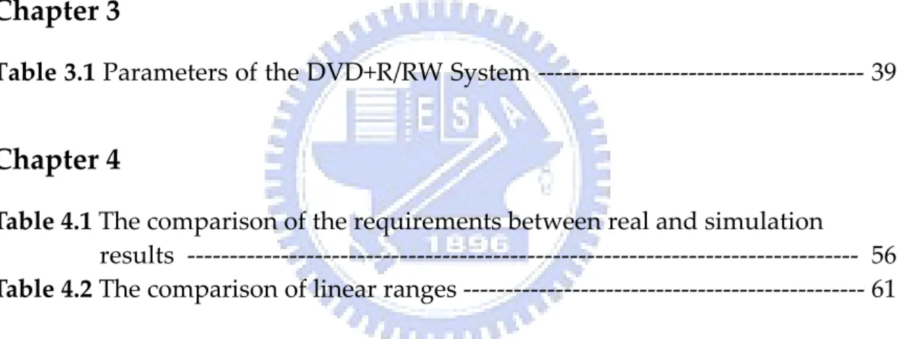
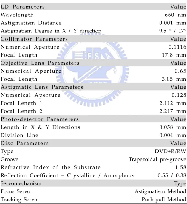
Table 3.1 Parameters of the DVD+R/RW System ‐‐‐‐‐‐‐‐‐‐‐‐‐‐‐‐‐‐‐‐‐‐‐‐‐‐‐‐‐‐‐‐‐‐‐‐‐‐‐ 39

Chapter 4

Table 4.1 The comparison of the requirements between real and simulation results ‐‐‐‐‐‐‐‐‐‐‐‐‐‐‐‐‐‐‐‐‐‐‐‐‐‐‐‐‐‐‐‐‐‐‐‐‐‐‐‐‐‐‐‐‐‐‐‐‐‐‐‐‐‐‐‐‐‐‐‐‐‐‐‐‐‐‐‐‐‐‐‐‐‐‐‐‐‐‐ 56 Table 4.2 The comparison of linear ranges ‐‐‐‐‐‐‐‐‐‐‐‐‐‐‐‐‐‐‐‐‐‐‐‐‐‐‐‐‐‐‐‐‐‐‐‐‐‐‐‐‐‐‐‐‐‐‐‐ 61

(15)

Chapter 1 Introduction

1.1 Motivation

As the coming of the tera‐era, the demand of the recording capacity is increasing. The areal density is governed by the numerical aperture (NA) and the wavelength (λ) of the optical pick‐up head (PUH). An optical data storage (ODS) system is developed toward a shorter wavelength laser diode and a higher numerical aperture objective lens, where the focused spot diameter is proportional to λ/NA, to achieve a higher areal density, as shown in Fig. 1.1‐1.

Fig. 1.1‐1 A diagram of the light paths for the CD, DVD and DVR system and

electron microscope photographs of the information pits of the three systems[1]

The optics of the ODS system including the fundamental principles of each optical component, disk recording are introduced in many literatures.

(16)

[2][3][4]_{These theories describe the propagation of the light in the optical}

pick‐up head, the interaction between the light and the media and the extraction of the readout and servo signals from the photo‐detectors. The literatures in this field primarily based on the geometry optics and the scalar diffraction theory proven to successfully characterize most of the observed phenomena.

When NA of the objective lens is higher than 0.6, the vector nature of the light field plays an important role in the optical readout process. The vector diffraction is needed to accurately model the interaction between the polarized light and the storage media. Because the calculation of the model based on vector diffraction theory is concerning with the interaction between the polarization of the light and the optical components, the cost of such model is extensive computation resources, such as the long computing time and the large memory capacity. Notwithstanding, to attaining acceptable levels of performance and reliability in the oncoming high‐NA optical data storage system, the simulation model based on the vector diffraction theory is indispensable and has been proposed by many research groups.[5]

The compromising method is combining the ray‐tracing and the vector diffraction model. The beam is traced through the entrance pupil of the ODS system, the objective lens, working distance and the disc substrate to the focal point. Near the focus the rays are transformed to the diffraction calculation. After reflected from the disc, the beam propagates a distance to a region where the ray‐tracing is valid once again.

A typical method to model the diffraction effect from the optical disc is to use a mark structure described by the Fourier series expansion in two

(17)

dimensions or by the fast Fourier transform algorithm. These methods can accurately estimate the optical phenomena in the optical data storage system, but have a less insight into the physics of the signal generation.

A different method called the Babinet principle which is based on the decomposition of the returning beam from a simplified disc structure is introduced to provide a physical insight into the diffraction mechanism of the optical readout system.[6]_{The Babinet principle is adopted in the proposed}

model to decompose the reflected light from the information layer of the disc into separate components that compose of the data signal, servo signals, and crosstalk so that the insight into the origin and the characteristics of various signals can be comprehended.

(18)

1.2 Objectives

Based on the Babinet principle and the vector diffraction theory, the objectives of this thesis are to simulate the readout signal and the servo signals including focus‐error signal (FES) and tracking‐error signal (TES) in the first stage. These signals are quantitatively compared with the specification requirements to verify the validity of the results.

In the following stage, the tolerance analysis including tilt and defocus of the key components are analyzed. Furthermore, tolerance experiments based on the DVD‐system will be implemented to verify the proposed model and demonstrate the feasibility.

In the final stage, the effect of feedthrough, the interaction between the two servo signals, are introduced and the discussion of the causes and the influence on the servo signals are presented.

(19)

1.3 Organization of This Dissertation

This thesis is organized as following: the basic principles and the prior studies utilized for constructing the model is reviewed in Chapter 2. In

Chapter 3, the simulation model and system configuration are proposed and

described. The simulation results including the readout signal, the servo signals, the tolerance analysis, and the effect of feedthrough is demonstrated and discussed in Chapter 4. The conclusion and the future works are given in

(20)

Chapter 2 Principles and Literature Review

In Chapter 2, the theories of the scalar and vector diffraction in the optical date storage system and the preliminary principles of decomposing the light reflected from the disc structure are reviewed; moreover, the fundamentals of the servo mechanism is described at the end of Chapter 2.

2.1 Scalar and Vector Diffraction Theory

Scalar diffraction theory is employed in the analysis, when the following two conditions are satisfied: (1) the NA is lower than 0.6; (2) the size of details on the disc are larger than the magnitude of the light wavelength (λ) employed. Because the bending of the rays by the focusing element is fairly small, the electromagnetic fields before and after the element to have a more or less the same orientations. However, when the optical system with a severe bending of the light rays, such as a high‐NA system, is adopted, the polarization effects of the light should be significant. The applicability of the scalar diffraction theory is based on the easy evaluation by the method of stationary phase approximation. In the stationary phase approximation, the plane wave spectrum of the convergent beam at the exit pupil is equivalent to the light amplitude distribution at that pupil; therefore, each geometric ray represents one plane wave of the spectrum.

(21)

2.1.1 Scalar Diffraction Theory [7] The Huygens‐Fesnel principle can be written ξ η ξ λ =

∫ ∫

₂01 ( , ) ( , ) jkr z e U x y U d d j _Σ r₀₁ η (2.1-1)

y

x

z

r

01

P

0

P

1

ξ

λ

z = Z

z = 0

η

Fig. 2.1‐1 Diffraction geometry

where the distance r01 is given by r₀₁ = (x−ξ)2+(y−η)2+z . As shown in 2

Fig. 2.2‐1, the diffraction aperture lies in the (ξ,η) plane, and is illuminated in the positive z direction. By the paraxial assumptions, (2.1‐1) becomes π _ξ _η λ ξ η λ ∞ _⎡ ₋ ₊ ₋ _⎤ ⎣ ⎦ −∞ =

∫ ∫

( ) (2 ) 2 ( , ) ( , ) jkz _j _x _y z e U x y U e d d j z ξ η (2.1‐1) and another form of (2.1‐1) is π π _ξ _η π _ξ _η λ ξ η λ λ ξ λ ∞ + + − −∞ ⎡ ⎤ = _⎢ _⎥ ⎣ ⎦

∫ ∫

2 2 2 2 2 ( ) ( ) ( ) ( , ) ( , ) jkz _j _x _y _j _j _x _y z z z e U x y e U e e d d j z η + (2.1‐2)

(22)

which is the Fourier transform of the product of the complex field and a quadratic phase term. (2.1‐1) and (2.1‐2) is the Fresnel diffraction (Near field) integral. If the phase term in the brackets of (2.1‐1) approaches unity, i.e. π _ξ _η λ

π ξ η

λ

+ ≈ ⇒ + << >> 2 2 2 ( ) ₂ ₂ max 1 ( ) 1 z j z D e o z r where the D represents the maximum dimension of the aperture, the observed field is the Fourier transform of the aperture. π π _{ξ η} λ _{ξ η} λ λ ∞ + − + −∞ = ( 2 2 )

∫ ∫

2 ( ) ( , ) ( , ) jkz _j _x _y _j _x _y z z e U x y e U e d d j z ξ η (2.1‐3) This is the Fraunhofer (Far field) diffraction integral where λ = x u z, v= yλz.

Except the phase factor preceding the integral, this expression is simply the Fourier transform of the aperture.

{

}

λ λ ξ η = = = ∗ , ( , ) ( , ) | _x _y u v z z U x y C F U (2.1‐4) where π λ λ + = ( 2 2) jkz _j _x _y z e C e j z and F represents the Fourier transform operation. There is an analogue method to determine the diffraction patterns after propagating through a distance called the angular spectrum of plane waves. Any complex amplitude distribution of the light can be decomposed into a spectrum of plane waves. The plane waves travel in different directions across the system, and then are superimposed to form a diffraction pattern at the destination plane.

(23)

In the ODS system, the light source is the laser diode which has a Gaussian complex amplitude distribution. The following of this section try to use this amplitude distribution to derive the diffraction formulas and compare this to the aforementioned theory. Generally, the Gaussian beam propagates along the z‐axis has the following complex amplitude distribution:

(

α β = − 2− 0 ( , ) exp U x y U x y2

)

_(2.1‐5)

In (2.1‐5), α and β are complex numbers. Consider the Fourier transform and corresponding inverse Fourier transform of such amplitude distribution at the z = 0 plane:

{

}

∞ π

(

)

−∞ ⎡ =

∫ ∫

_⎣− + ( , ,0) ( , ,0) exp 2 F U x y U x y j xu yv dxdy⎤⎦ ⎤ + _⎦ ＊ (2.1‐6)

{

}

π

(

)

∞ −∞ ⎡ =

_{∫ ∫}

_⎣ ( , ,0) ( , ,0) exp 2 U x y F U x y j xu yv dudv (2.1‐7) The right side of (2.1‐7) is the superposition of plane waves propagating long the unit vector σ , where σ = _ˆ+ _ˆ+ − 2− 2 1 u x v y u v zˆ (2.1‐8) ＊ The evaluation of the integral: ( ) π π π α β αβ ∞ −∞ ⎡ ⎛ ⎞⎤ ⎡− + ⎤ = _⎢− _⎜ + _⎟_⎥ ⎣ ⎦ _⎣ _⎝ _⎠_⎦

(24)

The amplitude of the propagating plane wave are the Fourier transform of the with the frequency (u,v). The plane waves propagate along the z‐axis from the origin to the z=Z plane, and the resulting distribution at the z=Z plane is obtained by the superposition of these plane waves after traveling a Z distance. ( , ) U x y

{

}

{

π

(

)

}

∞ −∞ ⎡ ⎤ = _⎢ + + − _⎥ ⎣ ⎦

∫ ∫

2 2 ( , , ) ( , ,0) exp 2 1 U x y Z F U x y j xu yv Z u −v dudv (2.1‐9)

A method called stationary‐phase approximation can be utilized to evaluate the integral value of (2.1‐9). [7][8]_{Consider a two‐dimensional integral}

[

]

ξ η κφ ξ =

∫∫

( , )exp ( , ) I f j x y d dη (2.1-10)

where f( , )ξ η is a complex function, and φ ξ η

(

,

)

is a real function, and κ is a large real number, and the domain of the integration .is a subset of the ξη‐plane. The small variation of the function φ ξ η

(

,

)

will be amplify by the large real number , and result in the rapid oscillation of the phase term. On the other hand, the complex function

κ

ξ η ( , )

f is a slow variation function which has a negligible effect on the integral. The main contribution of this integral is from the regions in the neighborhood of the stationary point of

(

)

φ ξ η, which is defined as (2.1‐11)

(25)

(

)

(

)

φ ξ η φ ξ η ∂ ₌ ∂ ∂ 0, 0 ∂ 0, 0 x y = 0 (2.1‐11) The integral in (2.1‐10) can be approximated as

[

]

[

]

ξ η κφ ξ η ξ η πν _{ξ η} _{κφ ξ η} κ αβ γ = ≅ −

∫∫

0 0 0 0 2 ( , )exp ( , ) 2 ( , )exp ( , ) I f j d d j f j (2.1‐12) where αβ γ α φ φ φ α β γ ν αβ γ α ξ η ξ η αβ γ ⎧ ∂ ∂ ∂ ⎪ = = = = −_⎨ ∂ ∂ ∂ ∂ _⎪− ⎩ 2 2 2 2 2 2 2 2 1, > , >0 1, > , <0 , < j (2.1‐13) When the real function φ ξ η

(

,

)

has the form

(

)

φ ξ η −ξ2 −η2 + ξ+ η , = 1 A B (2.1‐14) where A and B are real numbers. The integral in (2.1‐10) can be approximated as follow:

ξ η

κ

ξ

η

ξ

η

ξ

π

κ

⎡

⎤

=

_⎣

−

+

_⎦

−

_⎡

_⎤

≅

_⎣

−

_⎦

∫∫

2 2 2 2

( , ) exp

( 1

)

2 ( , ) exp

1

s

I

f

j

A

B

d d

j

f A B

j

A

B

η

(2.1‐15) ⎛ ⎞ ⎜ ⎟ + + + + ⎝ = + + 2 2 2 2 2 2 , 1 1 ( , ) 1 s A B f ⎠ A B A B f A B A B (2.1‐16)

(26)

where f A B_s( , ) is a stretch version of f( , )ξ η . Comparison of (2.1‐9) with (2.1‐15) shows that the two integrals are identical supposed that one makes the following associations:

{

}

κ π ξ η → = = = ( , ) ( , , 0) ; 2 ; ; f u v F U x y z z A B Z = Z

Consequently, the integral in (2.1‐9) is an approximated form by the stationary‐phase method as (2.1‐16):

{

}

ξ η π = = − _⎡ _⎤ ≅ _⎣ 2+ 2+ 2_⎦ ( , , ) exp 2 ( , , 0) A Z B Z s = j U x y Z j x y Z F U x y z Z (2.1‐17)

This is the fundamental equation of the scalar diffraction theory in the far‐field regime. The exponential term in (2.1‐17) is the curvature phase representing a radius of curvature Z. The stretching operation must be put on the function before Fourier transformation. Comparison of the approximated result (2.1‐17) with the far‐field integral (2.1‐3) demonstrates the consistency.

2.1.2 Vector Diffraction Theory [3][4]

The simple treatment of the effects concerning the polarization will be introduced in this section. Replacing the rigorous solution of the Maxwell’s equations with the physical phenomenon of bending of the plane wave by high‐NA lens is an intuitive approach about the propagation of the electromagnetic waves.

(27)

Incident Beam

E

Focus

E

X

Y

Z

Fig. 2.1‐2 A linearly polarized beam is brought to focus by a lens. The E‐field is the electric field indicating the direction of the polarization.

Consider a linearly polarized beam propagates along the z direction, as shown in Fig. 2.1‐2. The incident direction of propagation is σ0 =(0, 0,1), and

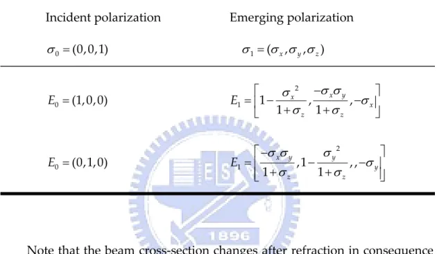
the corresponding direction of propagation after the lens is σ₁ =(σ σ σ_x, _y, _z). The incident polarization electric E₀ =(1,0,0) can be decomposed into two components, s‐polarization and p‐polarization. The s‐polarization is in the plane of the σ₀ and σ₁, and remains in the same direction of incidence after passing through the lens. In the meanwhile, the p‐polarization reorients to the perpendicular direction of the emergent rays. If the refraction process is lossless, the simple geometry is used to determine the new emerging polarization. Given the direction of incident beam σ₀ and the direction of the emergent beam σ₁, the polarization of the emergent beam can be resolved with the arbitrary polarization state of the incident beam, as listed in Table 2.1.

(28)

A similar calculation can be derived in the same procedure from an incident beam with polarization along y‐axis.

Table 2.1 The polarization of the emergent beam is E1, and the original polarization is E0 under the assumption of lossless refraction. Incident polarization Emerging polarization σ₀ =(0,0,1) σ₁ =(σ σ σ_x, _y, _z) = 0 (1,0,0) E σ σ σ σ σ σ − ⎡ ⎤ =_⎢ − − _⎥ + + ⎣ ⎦ 2 1 1 , , 1 1 x y x x z z E = 0 (0,1,0) E σ σ σ σ σ σ ⎡− ⎤ =_⎢ − − _⎥ + + ⎢ ⎥ ⎣ ⎦ 2 1 ,1 , , 1 1 x y y y z z E Note that the beam cross‐section changes after refraction in consequence of plane wave refraction. The cross‐section propagate along σ₁ is reduced by a factor σ_z, and therefore, its amplitude is increased by a factor 1_σ

z . The

correct emerging polarization amplitude is 1_σ

z

E _.

According to (2.1‐17), the amplitude distribution is Fourier‐analyzed across any plane, and the various spatial Fourier components can be identified as plane waves traveling in different directions. The amplitude at any point can be determined by superposing the constituent plane waves to join the phase shift obtained during propagation. Incorporating the polarization state of Table 2.1 with (2.1‐17) to get the formula for vector diffraction:

(29)

{

}

{

}

(

)

σ σ σ σ σ σ σ σ σ σ σ σ σ π σ σ σ σ σ ⎛ ⎞ − − ⎜ ₊ ⎟ + ⎜ ⎟ ⎛ ⎞ _⎜ _⎟ ⎜ ⎟₌ _⎜ ₋ ₋ _⎟ ⎜ ⎟ _⎜ ₊ ₊ _⎟ ⎜ ⎟ ⎝ ⎠ ⎜ ⎟ ⎜ ₋ ₋ ⎟ ⎜ ⎟ ⎝ ⎠ ⎛ = ⎞ ⎡ ⎤ ⎜ ⎟ × _⎣ + _⎦ ⎜ = ⎟ ⎝ ⎠

∫∫

2 2 1 1 1 ( , , ) 1 ( , , ) 1 1 1 ( , , ) ( , , 0) exp 2 ( , , 0) x y x z z x x y y y z z z z x y x x y z x y U x y z U x y z U x y z F U x y z + _y j x y z d d F U x y z (2.1‐18) and (2.1‐18) is the vector version of (2.1‐17) 2.1.3 Comparison The simplest focusing theorem is based on the scalar diffraction and the paraxial approximation. This simplest theorem is applicable only when the numerical aperture of the lens is low/moderate. When the NA of the lens up to the scale of which the polarization effect can not be neglect, the focusing problem should be dealt with the vector diffraction theory.

In this section, the author try to demonstrate the objective lens with different NA (NA=0.45, 0.85) to observe the intensity distributions in different polarization directions on its focal plane. The light is an x‐polarized Gaussian beam, and is incident to the lens with NA of 0.45 (CD) or 0.85 (DVR). The aforementioned vector and scalar diffraction theory are employed.

(30)

(a)

(b)

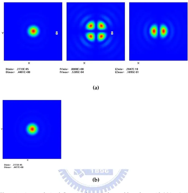
Fig. 2.1‐3 An x‐polarized Gaussian beam is focused by a lens with NA = 0.45, and observe the intensity distribution of X‐, Y‐, and Z‐polarization (from the left to the right) on the focal plane. The calculation method is (a) vector diffraction theory, and (b) scalar diffraction theory.

The x‐ and y‐axis in Fig. 2.1‐3 and Fig. 2.1‐4 are the coordinates in the focal plane and range from ‐5λ to 5λ. The intensity distributions in Fig. 2.1‐3(a) and Fig. 2.1‐4(s) are X‐, Y‐, and Z polarizations. There is only one plot in Fig. 2.1‐3(b) and Fig. 2.1‐4(b) because the scalar diffraction theory does not take polarizations into consideration.

(31)

(a) (b) Fig. 2.1‐4 An x‐polarized Gaussian beam is focused by a lens with NA = 0.85, and observe the intensity distribution of X‐, Y‐, and Z‐polarization (from the left to the right) on the focal plane. The calculation method is (a) vector diffraction theory, and (b) scalar diffraction theory.

As shown in Fig. 2.1‐3(a) and 2.1‐4(a), in y‐polarization four peaks occur near the focus, and in the z‐direction two peaks appear under the vector diffraction calculation. The summary of the maximum intensities along each direction and their comparisons are shown in Table 2.2.

(32)

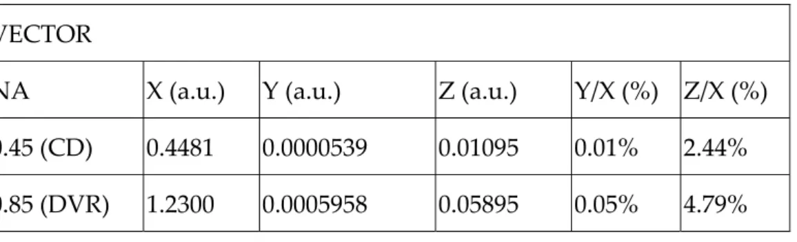
Table 2.2 Maximum intensities along x‐, y‐, and z‐direction and their comparisons

VECTOR

NA X (a.u.) Y (a.u.) Z (a.u.) Y/X (%) Z/X (%) 0.45 (CD) 0.4481 0.0000539 0.01095 0.01% 2.44% 0.85 (DVR) 1.2300 0.0005958 0.05895 0.05% 4.79%

In the case of NA = 0.45, the ratio of the peak intensity between Y and X‐direction is 0.01% which can be neglected and so does that of NA = 0.85. For the case of NA = 0.85, the ratio of the peak intensity between Z and X‐direction is 1.96 times larger than that in the case of NA=0.45 and is 95.8 times larger than that in the Y‐direction of the NA = 0.85. For this reason, the diffraction component in the Z‐direction can not be omitted any more while the NA of the objective lens is large enough.

(33)

2.2 The Babinet Principle [5][9]

The traditional way to model the propagation and interaction of the light in the ODS system is use a Hopkins‐type method in which the mark structure is expressed by the Fourier series expansion.[2]_{This model has a good estimate}

of the light, but has a less comprehension about the physics of the signal generation. The Babinet principle can provide quantitative results of the diffraction mechanism by decomposing the reflected field from the recording layer of the disc into ingredient components; these components with different combination form the readout signal, servo signals, and the crosstalk, respectively.

Objective Lens

Disc

Objective Lens

~ T

U

T

U

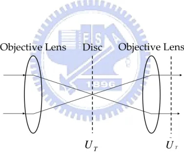
Fig. 2.2‐1 Light is focused on the disc and formed a reflected field .

The reflected field diffracts to form a field at the pupil of the objective lens. ( , ) T U x y ~ ( ', ') T U x y 2.2.1 Mathematical Formulations and Physical Description Consider a model which the objective lens focus the incident light onto the

(34)

recording layer of the optical disc and the light is recollimated by the objective lens, accordingly, as shown in Fig. 2.2‐1. The total light field reflected from the disk is , where the x and y represent the coordinates in the plane of the recording layer. The reflected beam is collimated by the objective lens and form a light field at the exit pupil of the objective lens, where the x’ and y’ represent the coordinates at the pupil. ( , ) T U x y ~ ( ', ') T U x y

The Babinet principle assumes that the total field reflected from the recording layer is the summation of the fields reflected from the separate regions. = = =

∑

1 i N T i

U

i i i (2.2‐1) i

U are the non‐overlapping composing regions on the optical disc. The summation of N components cover entire domain of . Linear operations performed on is a summation of the linear operation of each component . ( , ) T U x y ( , ) T U x y U = = =

∑

~ ~ 1 i N T i

U

(2.2‐2) The tilde refers to the linear operation of the propagation from the disc plane to the exit pupil of the objective lens.

(35)

different marks of two adjacent tracks, T1 and T2, as depicted in Fig. 2.2‐2. The laser spot focused on the recording layer scans over track T1 with an offset yΔ . The marks on T1 and T2 are denoted as M1 and M2, respectively. The track pitch is indicated by P.

T1

T2

Δy

Laser Spot

_{On-track Marks}

Off-track Marks

Fig. 2.2‐2 Track layout of the disc

Each component of include the three parts: (1) the electric field reflected from mark M1 of track T1, i U 1 M U ; (2) the electric field reflected from mark M2 of track T2, U_M₂; (3) the electric field reflected from the land, . The Babinet principle declare the total reflection from the recording layer as i U T U

=

+

(

−

)(

₁

+

T L F M L M M

U

r U

r

U

2

)

(2.2‐3)

where the rL and rM are the complex reflectance of the land and the mark,

respectively, and is the reflection form the flat surface of the disc, as illustrated in Fig. 2.2‐3.

F

U

(36)

=r_L* + r_M* UM = UM1 + UM2 U_L r_M r_L =r_L-* U_M =r+ r_L_M** U_M U_M= U_M1+ U_M2 = r_L* U_F U_F = r_L* = r_L* + (r_M-r_L)* U_T Fig. 2.2‐3 The Babinet principle used to decompose the signal reflected by the optical disc

The ingredients UM1 and UM2 are binary value with a maximum of one and

a minimum of zero. Take the groove structure into account, the flat reflection term, U_F transform to the form U_F = exp[ ( , )]i xφ y , where the φ( , )x y represents the phase imported by the grooves as a function of the position on the recording layer.

2.2.2 Generating the Readout, Servo, and Crosstalk

The total field at the exit pupil of the objective lens, , propagate to the detector that generate the date signal and the servo signals. The data signal reveals the mark distribution beneath the scanning laser spot; the servo signal

~

T

(37)

is sensible to the offset . The crosstalk between the data channels is caused by the interaction between the rim of the focused laser spot and the adjacent tracks. The reflection from the on‐track mark,

Δy

~ 1

M

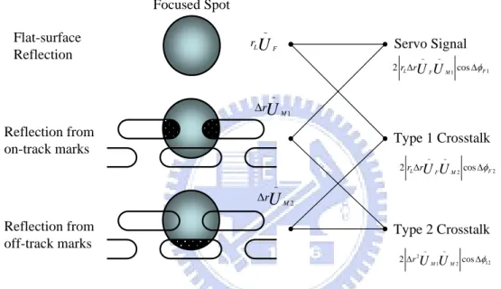
U , are important factor for analysis. U~ _M₁ shows the symmetry in the amplitude and the phase along the track direction when the laser spot scans over the mark M1. Focused Spot Flat-surface Reflection Reflection from on-track marks Reflection from off-track marks ~ 1 M r_U Δ ~ 2 M r_U Δ ~ L F r_U ~ ~ 2 2 2r rLΔU UF M cosΔφF ~ ~ 2 12 1 2 2Δr_{U U}_M _M cosΔφ ~ ~ 1 1 2rLΔrU UF M cosΔφF Type 1 Crosstalk Servo Signal Type 2 Crosstalk

Fig. 2.2‐4 Different combinations of the reflection terms generate the servo signal, and two types of crosstalks

The amplitude diffraction pattern splits and the phase of the amplitude diffraction pattern rotates when the laser spot scans over an on‐track mark. The rotation of the phase is due to the linear phase term has been introduced into the reflection field during scanning the off‐track marks. The component fields, , , and with different combinations form the data signal, servo signals, and crosstalks, as illustrated in Fig. 2.2‐4.

~ ~ ~

F

U UM1 UM2

(38)

from the flat reflection, , combines with the diffraction from the on‐track marck, , to form the servo signal: ~ F L r U ΔrU~F φ Δ ~ ~ ₁ ₁ 2r rL

U U

F M cosΔ F (2.2‐4)

where Δ =r rM −rL and ΔφF1 is the phase difference between the two constructed components. Secondly, the type one crosstalk: φ Δ ~ ~ ₂ ₂ 2 r rL

U U

F M cosΔ F (2.2‐5) , is formed by the flat reflection and the diffraction from the off‐track marks. Lastly, the diffraction from the on‐track and the off‐track mark lead to a type two crosstalk: φ Δ 2 ~ ~ 12 1 2 2 r

_{U U}

_M _M cosΔ (2.2‐6)

A summary of the terms generated by the different combinations of the diffraction terms and its physical explanation is listed in Table 2.3. The detector responds to the irradiance of the light field, ∝

2

~ ~

T T

I U . The servo current is formed by integrating the irradiance of the resulting diffraction term: φ Ω =

_∫

2 Δ ~ ~ ₁ cosΔ ₁ ʹ SERVO L F M F I r r

_{U U}

dx dyʹ (2.2‐7) where is the area of the pupil aperture. The data signal is determined by the same way: Ω

(39)

2 ~ 1 ' DATA M ' I r

_U

dx dy Ω = Δ

∫

(2.2‐8) Table 2.3 The diffraction terms resulting from the Babinet decomposition [5] Diffraction Terms Formula Physical Description

Background 2 ~ L F r

_U

Background reflection Data Signal Δ 2 ~ 1 M r

_U

Interference of the M1 with itself Type 0 crosstalk Δ 2 ~ 2 M r

_U

Interference of the M2 with itself Servo Signal _Δ ~ ~ _φ 1 1 2r rL

U U

F M cosΔ F Interference of the M1 with background Type 1 crosstalk _Δ ~ ~ _φ 2 2 2r rL U UF M cosΔ F Interference of the M2 with background Type 2 crosstalk Δ 2 ~ ~ _φ 12 1 2 2 r

_{U U}

_M _M cosΔ Interference of the M1 and the M2 2.2.3 Applications of the Babinet principle In this section, the two applications of the Babinet principle is introduced. The first application is the explanation of the origin of the differential phase detection (DPD) method, which is used as a tracking method to maintain the laser spot on the target track. The DPD tracking signal originates from the rotation of the diffraction pattern which been detected by the quadrants of the detector.

Case I : r_L≠ 0,r_M = 0, without grooves and one isolated mark,M1

應用於高密度光儲存系統讀取信號之模擬

國

立

交

通

大

學

光電工程研究所

碩士論文