打光與霧特效的轉移

國

立

交

通

大

學

多媒體工程研究所

碩

士

論

文

打

光

與

霧

特

效

的

轉

移

Lighting and Foggy Effect Transfer

研 究 生：黃富熙

指導教授：莊榮宏 教授

林文杰 教授

打光與霧特效的轉移

Lighting and Foggy Effect Transfer

研 究 生：黃富熙 Student：Fu-Hsi Huang

指導教授：莊榮宏 Advisor：Jung-Hong Chuang

林文杰 Wen-Chieh Lin

國 立 交 通 大 學

多 媒 體 工 程 研 究 所

碩 士 論 文

Submitted to Institute of MultimediaEngineering College of Computer Science

National Chiao Tung University in partial Fulfillment of the Requirements

for the Degree of Master

in

Computer Science

September 2014

Hsinchu, Taiwan, Republic of China

Lighting and Foggy Effect Transfer

Student: Fu-Hsi Huang

Advisor: Dr. Jung-Hong Chuang

Dr. Wen-Chieh Lin

Institute of Multimedia Engineering

College of Computer Science

National Chiao Tung University

ABSTRACT

Rendering participating media plays an important role in animation or games, since it can influ-ence the atmosphere of scenes and generate some special lighting effects such as the glow and god rays. To design a scene with participating media such as fog and glow effects, it usually require user to fine tune some parameters of lighting and fog to achieve their goal. We propose a method that aims to transfer the desired lighting and foggy effect on a photo to the 3D scene by solving an inverse problem. We can generate a 3D scene with similar specified effects and atmosphere on the target image. Computation time depends on the complexity of the input scene.

Acknowledgments

I would like to thank my advisors, Professor Jung-Hong Chuang, and Professor Wen-Chieh Lin for their guidance. I also want to thank Tsung-Shian Huang for his comments. Lastly, I am grateful to the support from my family in these years.

Contents

1 Introduction 1 2 Related Work 3

2.1 Lighting Design . . . 3

2.2 Participating Media Design . . . 7

3 Volume Rendering 9 4 Lighting and Foggy Effect Transfer 12 4.1 System Overview . . . 12

4.2 User control . . . 15

4.3 Optimization . . . 17

4.3.1 Problem Formulation . . . 18

4.3.2 Compute Optimal Configuration . . . 19

4.4 Rendering System . . . 20

4.4.1 Rendering Equation . . . 21

4.4.2 Ray-Casting Implementation . . . 21 5 Results 23 6 Conclusion and Future Work 33

Bibliography 34

List of Figures

2.1 Galleries system [7]. The upper half is configuration generated by the system. The lower right is configuration selected by the user. The lower left is the optimal result. . . 4 2.2 Illuminaiton brush [9]. (a) User paint on the object directly. (b) Compute the

environment light and store in an environment map. . . 4 2.3 Lighting with paint [10]. (a) User paint on the object directly. (b) Compute the

setting configuration. . . 5 2.4 Interactive lighting design [6]. (a) The user draws shadow strokes. (b) Compute

the lighting setting based on the shadow strokes. (c)(d) The user adjusts details including shadow, color and intensity of lights. . . 6 2.5 Modeling clouds using photographs [2]. . . 7 2.6 Rendering clouds using photographs. Upper left image: photograph. Main

image: synthesized clouds [3]. . . 8 2.7 Volume stylizer [4]. . . 8 3.1 Single scattering and multiple scattering cases [1]. . . 9 3.2 Light transport going into eyes of the observer along the direction ω. It includes

the radiance scattered by air and the radiance reflected by the surface of objects. 10 4.1 Flowchart of our method. . . 14

4.2 Steps of drawing glow lines. Place a start point and and end point (a) to deter-mine the scope of the glow line. (b) and (c) are examples of a pair of patterns in the form of concentric circles for the scene image and target image, respectively. 15 4.3 Steps of drawing fog lines. Place a start point and an end point (a) to determine

the scope of the fog line. (b) and (c) are examples of a pair of fog lines for the

scene image and target image, respectively. . . 16

4.4 Steps of drawing ray lines. Place a start point and an end point to determine the scope of the ray line on brighter part of god rays for the scene image (a) and target image (c). Draw another pair of ray lines on the darker part of god rays for the scene image (b) and target image (d). . . 17

4.5 Step one: store the entry points of the volumetric data in the coordinate texture. Step two: compute directions of rays with the coordinate texture and start ray traversal. . . 22

5.1 The flowchart of our system when designing a scene. . . 24

5.2 Transfer the glow of the spotlight. . . 25

5.3 Transfer different parts of glow effect from the target image. . . 26

5.4 Transfer the glow effect from the same target image. . . 27

5.5 Transfer the fog effect. . . 28

5.6 Top row: design the scene by using only the glow line. Bottom row: design the scene by using the fog line and the glow line. . . 29

5.7 Design the scene with god rays. . . 30

5.8 Extract the atmosphere from the target image. . . 31

List of Tables

3.1 Symbols summary. . . 11 5.1 Optimization time of results. . . 32

C H A P T E R

1

Introduction

Participating media includes many natural effects, such as fog, mist and haze. Scattering in participating media can cause amazing phenomenon including god rays and glow. The scenes with participating media in animation and game usually have lighting effects, such as the glow lighting up the foggy street or god rays shining through trees in forest. To design a scene with these effects in participating media by using 3D animation software, users usually need to know the meaning of many parameters about lights and the participating media and then design in trial-and-error basis. It is a complicated process for the novices to adjust the parameters to obtain desirable results.

We propose an approach that is able to transfer the desired foggy and lighting effects on a target image to a 3D scene by solving an inverse problem, aiming to find a set of parameters with which the scene would have similar foggy and lighting effects as the target image. On the target image and the rendered scene image, users draw some control patterns that are used to constrain the sampling. The inverse problems tries to minimize the error metric between the target image and rendered scene image on samples drawn from the control patterns. As a result, a set of optimal parameters about lighting and fog is obtained.

The contributions of this thesis can be summarized as:

2 • The glow effect, god rays and foggy effect on the target image can be identified and

transferred to a 3D scene by solving an inverse problem.

• The required user interaction is very limited and intuitive. Only a few lines or patterns need to be specified by the user. User need not to know the parameters for lighting and foggy effects.

The rest of the thesis is organized as follows: Related work is reviewed in Chapter 2. Volume rendering equation is introduced in Chapter 3. The proposed method is illustrated in Chapter 4. The experiment results of the method are displayed in Chapter 5. Finally, conclusion and future work are discussed in Chapter 6.

C H A P T E R

2

Related Work

In this chapter, we review the literatures related to our study, including lighting design and participating media design.

2.1

Lighting Design

Several lighting design by painting have been proposed [12][7][6][9][10]. Schoeneman et al. first described a method to set lighting configuration with known light positions by solving an inverse problem [12]. The user paints on the 3D scene, and the intensities of lights can be derived automatically. Marks et al. proposed a design galleries system [7] providing an intuitive interface. The user chooses desired galleries rendered by configurations suggested by the system as targets, and then the optimal result similar to those targets is computed; see Figure 2.1.

2.1 Lighting Design 4

Figure 2.1: Galleries system [7]. The upper half is configuration generated by the system. The lower right is configuration selected by the user. The lower left is the optimal result.

The method proposed by Okabe et al. [9] generates the environment light automatically by solving an inverse shading problem to meet the painted illumination effects specified by the user; see Figure 2.2. It is an interactive lighting design due to the use of pre-computed radiance transfer. Although it can handle environment lighting design well, it cannot handle point lights.

(a) Painting (b) Setting configuration

Figure 2.2: Illuminaiton brush [9]. (a) User paint on the object directly. (b) Compute the environment light and store in an environment map.

2.1 Lighting Design 5 In the method presented by Pellacini et al. [10], the user paints color, light shape, shadows, highlights and reflections on the 2D image, and the optimal parameters of lights for meeting the desired illumination effects can be found; see Figure 2.3. Nevertheless, the method can only adjust one light at a time which is not well suited for scenes with many lights. The required painting is also inconvenient to the user who is unfamiliar with the knowledge of lighting.

(a) Painting (b) Setting configuration

Figure 2.3: Lighting with paint [10]. (a) User paint on the object directly. (b) Compute the setting configuration.

Lin et al. proposed an guiding system to specify lighting and shadow [6]. In the first step, positions and numbers of lights are determined based on shadow strokes drawn by the user. Some initial lighting conditions are precomputed, and an appropriate lighting configuration are computed by least square. Then they use Nelder-Mead simplex to solve better light positions with a light tree. Other details including color, intensity and shadow can be adjusted based on the result of the first step; see Figure 2.4. The method can handle multiple lights at once.

2.1 Lighting Design 6

(a) Assigning shadow (b) Computing lighting

(c) Erasing shadow (d) Adjusting details

Figure 2.4: Interactive lighting design [6]. (a) The user draws shadow strokes. (b) Compute the lighting setting based on the shadow strokes. (c)(d) The user adjusts details including shadow, color and intensity of lights.

2.2 Participating Media Design 7

2.2

Participating Media Design

Zhou et al. proposed an interactive design system for smoke or fog by incorporating their an-alytic method for handling isotropic, single-scattering media illuminated by point light sources [14]. The user paint on the 3D scene directly, and Gaussians are placed along the strokes painted by the user to model the distribution of media. Dobashi et al. proposed a method to synthesize clouds by analyzing the density distribution of clouds from an input photograph [2]; as shown in Figure 2.5. These two methods aim to design the distribution and the shape of the participating media, but do not control the lighting parameters.

(a) Input photograph (b) Result

Figure 2.5: Modeling clouds using photographs [2].

Dobashi et al. proposed a method that finds parameters for rendering clouds by using a reference photographs [3]; as shown in Figure 2.6. Giving a cloud density data and a photograph of real clouds, the rendering parameters are generated by using a genetic algorithm to minimize the difference between the color histogram of the synthesized image and the photograph. The final image rendered by the optimal parameters is visually similar to the input photograph. The problem is related to ours, but it is for clouds in the sky. The backgrounds of cloud and fog are quite different. For example, there are only clouds in the sky, but there are many things such as trees and buildings on the ground. The influence of the background must be considered. They do not handle the case of lights inside clouds because they just consider one light source, namely sun. In addition, god rays effect is not included in their method too.

2.2 Participating Media Design 8

(a) (b) (c)

Figure 2.6: Rendering clouds using photographs. Upper left image: photograph. Main image: synthesized clouds [3].

Klehm et al. proposed a method for stylizing volumetric data [4]. The user needs to paint on the images for different views of the volumetric data. Emission, albedo and extinction co-efficient of the volumetric data are derived to allow the rendered image close to those images drawn by the user. They reconstruct the rendering equation such that the emission, albedo and extinction are the solution of a linear system and then solve the linear system by least square. Their method is for solving a specific volume appearance like Figure 2.7(b), and lighting effects such as the glow and god rays in the volume data are not considered.

(a) Original volumetric data (b) Stylized result

C H A P T E R

3

Volume Rendering

We review the necessary knowledge about volume rendering used in our approach. Volume rendering consists of some physical processes including absorption, which is the loss light being converted to other energy, emission, which is additional energy from the luminous media, and scattering which is composed of in-scattering and out-scattering. In-scattering includes single scattering coming from light sources and multiple scattering reflected from other directions; as shown in Fig 3.1. Out-scattering is the light changing direction due to the collision with some particles. In the following paragraph, we introduce radiance transfer equation that represents how light interacts with the participating media.

Figure 3.1: Single scattering and multiple scattering cases [1].

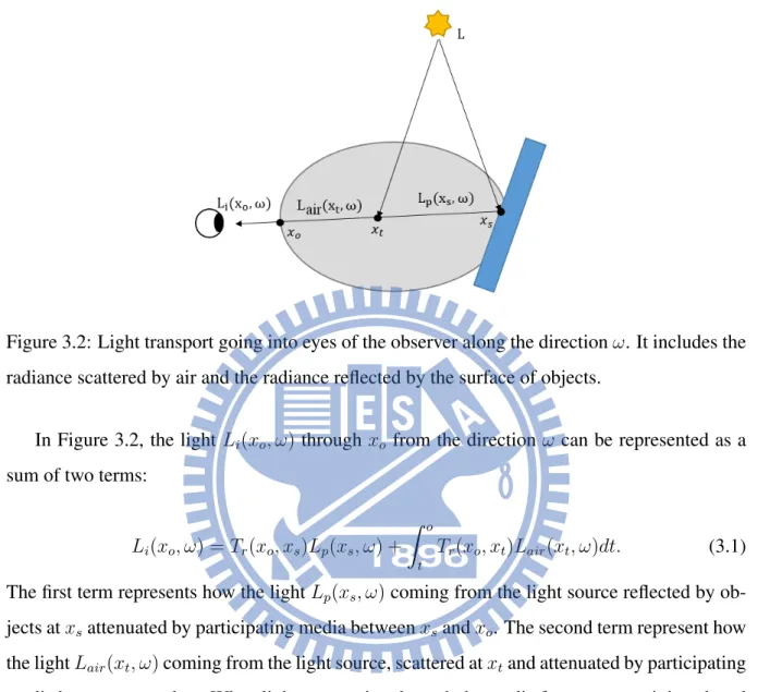
10

Figure 3.2: Light transport going into eyes of the observer along the direction ω. It includes the radiance scattered by air and the radiance reflected by the surface of objects.

In Figure 3.2, the light Li(xo, ω) through xo from the direction ω can be represented as a

sum of two terms:

Li(xo, ω) = Tr(xo, xs)Lp(xs, ω) +

Z o

t

Tr(xo, xt)Lair(xt, ω)dt. (3.1)

The first term represents how the light Lp(xs, ω) coming from the light source reflected by

ob-jects at xsattenuated by participating media between xsand xo. The second term represent how

the light Lair(xt, ω) coming from the light source, scattered at xtand attenuated by participating

media between xtand xo. When light penetrating through the media from xsto xo, it is reduced

due to the absorption and out-scattering. The transmittance Tr(xo, xs) is the ratio of the rest

light leaving the media between xoand xs:

Tr(xo, xs) = e− Rs

o σt(xu)du, (3.2)

where σt(x) = σa(x) + σs(x) is the extinction coefficient composed of absorption coefficient

σa(x) and scattering coefficient σs(x). The radiance Lair(xt, ω) in direction ω at point xt

11

Lair(xt, ω) = Lemit(xt, ω) + Lscat(xt, ω). (3.3)

Emission Lemit(xt, ω) increases the radiance at point xt, but it only happens when the medium

is luminous, such as fire and lightning within clouds. In-scattering Lscat(xt, ω) is the sum of the

radiance coming from other directions; i.e, Lscat(xt, ω) = σs(xt)

Z

Ω

f (xt, ω, ωl)Li(xt, ωl)dωl, (3.4)

where Li(xt, ωl) is incoming radiance at xtin direction ωland the outgoing radiance Li(xt, ωl)

in direction ω determined by the phase function f (xt, ω, ωl) that defines how much light in

direction ωlwill scatter to the direction ω after penetrating through xt. Integrating over the unit

sphere surrounding the point xt by applying Equation 3.1 recursively to gather in-scattering

results in Lscat(xt, ω). σs(xt) is the scattering coefficient for control the strength of scattering

effect at xt.

We summarize the symbols of volume rendering equation in Table 3.1. Symbol Description

σt(x) Extinction coefficient at x. σt(x) = σa(x) + σs(x).

σs(x) Scattering coefficient at x.

σa(x) Absorption coefficient at x.

f (x, ω, ωl) Phase function at x.

Tr(xo, xs) Transmittance between xo and xs.

Lp(xs, ω) Radiance reflected by the surface of the object.

Lair(x, ω) Radiance scattered by air.

C H A P T E R

4

Lighting and Foggy Effect

Transfer

In this chapter, we describe the algorithm of our system. Section 4.1 give an overview of our algorithm. Then we describe each part of our algorithm: user control (Section 4.2), optimization (Section 4.3), and rendering system (Section 4.4).

4.1

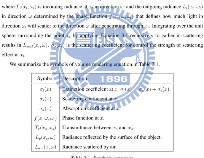
System Overview

This study aims to simplify the process of designing lighting and foggy effects in 3D scenes. In the forward methods, parameters of lighting and participating media are adjusted manually in trial-and-error basis until the desired result is reached, which is not an easy task for normal users since they may not know how the parameters related to the desired effects. In the backward or inverse methods, the desired effects or some references are provided, and then the optimized solution is found through an optimization algorithm which minimizes the difference between the desired effect and the synthesized result. In this study, we take the backward approach and use some lighting and foggy effect on a target image as the reference. The input of our system

4.1 System Overview 13 is a 3D scene and a target image It. Some control lines or patterns for sampling are drawn in

correspondence on the target image and the rendered image I(X0) of the 3D scene with default

setting X0 of the lighting and fog parameters. The control lines or patterns are denoted as St

and Ss, respectively for the target image and rendered image. Comparing correspondences on

Stwith Ss, the rendering parameter Xiis modified automatically until an appropriate parameter

X∗ is found. The 3D scene with the optimal lighting and fog parameters X∗ is the final output of our system.

Figure 4.1 illustrates the flowchart of the algorithm with the following major components: 1. User control

For effect transfer, we use an image such as a real photo that contains the desired lighting and foggy effects as the target image. Instead of sampling the whole image, the parts of the image that reveals the expected effects are sampled during the optimization. It is difficult to recognize the desired effects automatically, so the ones that reveal image having the desired effects are identified manually. On the target image and the rendered image of the input 3D scene, we draw control lines or patterns for the sampling used in the optimization process. The control lines or patterns include the glow line for extracting the glow effect, the fog line for extracting the foggy effect and the ray line for controlling the god rays. These control lines or patterns are used for sampling pixels on the target image and the rendered image.

2. Optimization

Our goal is to transfer the desired effects on the target image to the 3D scene. Thus the problem is to find a set of parameters X∗ with which the rendered image is as similar as possible to the target image on the selected effects. We regard this derivation as an optimization problem that can be solved by using Nelder-Mead simplex algorithm [8]. 3. Rendering system

We use volume rendering to render scenes with the participating media. Since the opti-mization is an iterative process and the 3D scene is rendered for each iteration. The

ren-4.1 System Overview 14 dering takes part of the optimization cost. To ensure an interactive design performance, we currently consider only homogeneous media with single scattering. In addition, we achieve real-time rendering for each iteration by using the GPU-based technique [5].

4.2 User control 15

4.2

User control

There are three types of controlling patterns used for representing how the desired effects are sampled. These controlling patterns are placed in pair on both of the target image and the rendered image of the input scene.

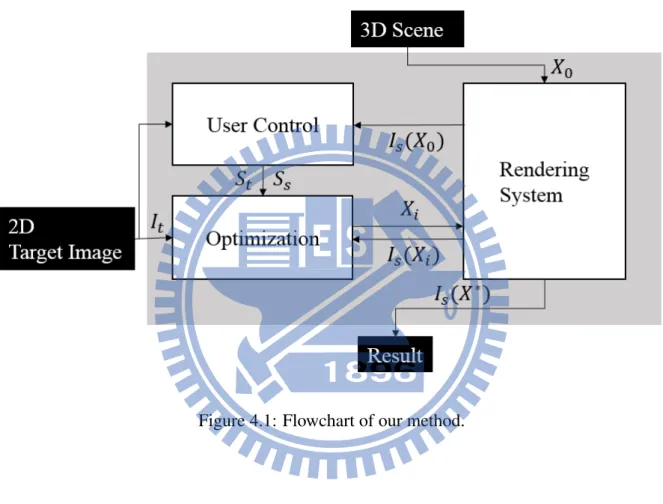
The first one is the glow lines for transferring the glow effect on the target image. Since the shape of glow for a point light source is almost a circle, we allocate sample points in a circular pattern to sample the variation of glow. That is, glow lines consist of sample points distributed in the pattern of concentric circles. Figure 4.2 depicts how the glow lines are placed on the scene and target image. In Figure 4.2 (a), a start point as the center of a circle and an end point representing the expected scope of the glow effect are placed first. Then sample points which distributed in a way of concentric circles are generated; see Figure 4.2 (b). Similar glow lines are placed on the target image; see Figure 4.2 (c).

(a) (b) (c)

Figure 4.2: Steps of drawing glow lines. Place a start point and and end point (a) to determine the scope of the glow line. (b) and (c) are examples of a pair of patterns in the form of concentric circles for the scene image and target image, respectively.

The second one is the fog lines for transferring the fog effect on the target image. The appearance of fog varies from far to near, so we draw a line that is able to depict the depth variation of the scene to sample this information. The example of using the fog line is shown in Figure 4.3. A start point and an end point are set to draw the fog line; shown in Figure 4.3(a)

4.2 User control 16 for the input scene image. Then sample points are generated within the line; see Figure 4.3(b). Similarly, a fog line is drawn on the target image; shown in Figure 4.3(c).

(a) (b)

(c)

Figure 4.3: Steps of drawing fog lines. Place a start point and an end point (a) to determine the scope of the fog line. (b) and (c) are examples of a pair of fog lines for the scene image and target image, respectively.

The third one is the ray line for transferring god ray effects on the target image. The god rays have different brightness because light rays are occluded by objects. Thus ray lines need to be drawn both on the darker part and the brighter part. Figure 4.4 show the example for the ray lines. A ray line is also generated by a start and a end point. When drawing ray lines on the scene image, the end point is placed by the user as shown in Figure 4.4(a). The start point is determined by the position of the light source. The line between the start and end points may extend to outside of the view, but only sample points in the view are considered. The ray line for the brighter part of god rays are drawn; see Figure 4.4 (a) and (c). The corresponding ray

4.3 Optimization 17 lines for darker part are placed on the scene and target image in similar way; see Figure 4.4 (b) and (d), respectively.

(a) (b)

(c) (d)

Figure 4.4: Steps of drawing ray lines. Place a start point and an end point to determine the scope of the ray line on brighter part of god rays for the scene image (a) and target image (c). Draw another pair of ray lines on the darker part of god rays for the scene image (b) and target image (d).

4.3

Optimization

The solution of this optimization problem is a set of optimal parameters including lighting and fog parameters. Lighting parameters include intensity and color of each light source. Fog pa-rameters consist of extinction σt, albedo ρ and a variable for approximating multiple scattering

4.3 Optimization 18 the scene can be seen clearly. Otherwise, the scene is sheltered by the fog. Albedo controls the scattering effect. When albedo is high, the scene is bright because of strong scattering. Extinction and albedo influence the amount of radiance through fog, and therefore they can be regard as the density of fog. Lm can prevent the scene form being too dark due to leaking of

multiple scattering. Because we assume that the media is homogeneous, the fog parameters are global variables.Lighting parameters of each light consist of color and intensity which control the appearance of glow and the brightness of the scene. Because the channel of color is three, each light has four dimensions. If the number of lights is Lnum, the total dimension of X is

(3 + 4 × Lnum).

4.3.1

Problem Formulation

The inputs of our system is a 3D scene with the default setting X0 for lighting and foggy

effects. A target image is selected, and controlling patterns for sampling on both target image and rendered scene image of the input scene are drawn. Our problem is to search for the optimal configuration X∗ with which the effect on the rendered image can be close to that on the target image as much as possible. We compute X∗by minimizing the objective function O defined as follows:

arg min

X

O(It, Is(X)), (4.1)

where X is a vector consisting of lighting and fog parameters, It is the target image for the

expected result and Is(X) is the scene image with parameter X. The objective function O

consists of Ef ogfor the foggy effect and Elightfor the glow effect and god rays defined as:

O(It, Is(X)) = αEf og(It, Is(X)) + βElight(It, Is(X)), (4.2)

where α and β are scalar weights.

When the distance to eyes is farther, light reaching eyes are less because of absorption and out-scattering of fog, and therefore the fog looks deeper. The scene becomes whiter because of

4.3 Optimization 19 deep fog. The variation of fog from near to far is close to the variation of saturation of HSV color space from 1.0 to 0.0. Thus we use saturation of HSV color space to display the fog variation. Saturation is independent of hue, so the influence from color with different hue of the background can be decreased. Thus Ef ogis used for sampling the difference of saturation along

the fog lines. That is,

Ef og(It, Is) = 1 Nf Nf−1 X i=0 kPs,i(It) − Ps,i(Is)k2, (4.3)

where Ps,i is saturation of the sample point i on the fog line and Nf is the number of sample

points.

Because the glow effect includes color and intensity of light, we use the color of pixel to display glow. God rays belong to the lighting effect, so it is defined by the same way as glow effect. Elightis the difference of color for samples on the glow lines or ray lines. That is,

Elight(It, Is) = 1 Ng Ng−1 X i=0 kPhsv,i(It) − Phsv,i(Is)k2, (4.4)

where Phsv,iis HSV for the sample point i on the glow line or ray line, and Ngis the number of

sample points.

4.3.2

Compute Optimal Configuration

We use Nelder-Mead simplex algorithm [8] to minimize Equation 4.1. Simplex is an optimiza-tion algorithm for minimizing the funcoptimiza-tion of n dimension. (n + 1) initial points X0, X1,...Xn

construct the initial simplex, where point has n dimension. Simplex adapt itself iteratively to find the local minimum X∗by replacing the point with a better one.

In the first step , the (n + 1) initial points need to be generated. Each point has the same dimension with X in Equation 4.1. The first point is the initial condition X0 which means the

setting of input. The rest of n initial points are generated by shifted each dimension of X0. The

color of light in initial points is determined based on the color of sample points in the glow line or the ray line.

4.4 Rendering System 20 The simplex is built according to the initial points. Then use these points to rendering scene images, and compute the error for each points by Equation 4.2. The point with highest error, Xh, will be replaced. There are three operations, namely reflection, expansion and contraction

involved in the replacement. The centroid of the points is defined as ¯X, and the reflection of Xh

is denoted by X_hr.

X_hr = (1 + α) ¯X − αXh, (4.5)

where α is reflection coefficient. If O(X_hr) < O(Xh) and O(Xhr) > O(Xl), where Xl is the

point with lowest error, then Xh is replaced by Xhr. If O(X r

h) < O(Xh) and O(Xhr) < O(Xl),

then expansion operation is used to compute Xeby

Xe= γXhr+ (1 − γ) ¯X, (4.6)

where γ is expansion coefficient. If O(Xe) < O(Xhr), then Xhis replaced by Xe. Otherwise, Xh

is still replaced by X_hr. When reflection failed, which means O(X_hr) > O(Xh), then contraction

operation is performed as follows:

Xc= βXh+ (1 − β) ¯X, (4.7)

where β is contraction coefficient and Xh is replaced by Xc. The algorithm repeats this step

until the point with the local minimum is found. The local minimum means that the scene image is close to the target image, so the parameters of the point is optimal configuration X∗.

4.4

Rendering System

The common technique for rendering participating media is ray marching which is time con-suming due to the complicated calculation of multiple scattering. Since the proposed optimiza-tion algorithm involves the scene rendering at each iteraoptimiza-tion, the rendering must be in real time. Thus we employ only single scattering and use the method proposed by Kr¨uger et al. [5] to accelerate the ray casting process.

4.4 Rendering System 21

4.4.1

Rendering Equation

The parameter Lprepresenting the light reflected by objects is modeled by Phong model:

Lp(xs, ω) = kaLa+

1

kd2(kdLd(l · n) + ksLs(r · ω)

ns_{)), (4.8)}

where n, r, l and ns are the normal of the surface, reflected light, light direction and surface

roughness, respectively. kaLa, kdLdand ksLsare ambient light, diffuse light and specular light,

respectively. k is attenuation factor which simulates the light attenuation due to the distance d. We consider only single scattering effect, and use a constant Lm to approximate the effect

of the multiple scattering. In addition, we assume that the media is non-luminous such as fog, so Lemitfor luminous media can be ignored. Therefore, in the Equation 3.3 Lair(xt, ω) is

Lair(xt, ω) = Lss(xt, ω) + Lm. (4.9)

The single scattering that directly comes from the light and goes through point xt in the

direction ω is

Lss(xt, ω) = σs(xt)f (xt, ω, ωl)L, (4.10)

where f (xt, ω, ωl)), a phase function, is assumed to be isotropic in our study, and ωl is the

direction from the light to xtand L is the intensity of the light source.

4.4.2

Ray-Casting Implementation

There are many ways of implementing the volume rendering. The method we choose is ray casting. Ray casting is the method that casts a ray along the view direction through each pixel, and integrates lighting of voxels along the ray. The rendering process is composed of many fragment operations that include lighting computation, so reducing cost of per-fragment op-erations can also accelerate the rendering process. Kr¨uger et al. [5] proposed a GPU-based technique to accelerate fragment operation. Two steps are involved. In step one, they render

4.4 Rendering System 22 front face of the volumetric data for obtaining the entry points, and store the entry points in a coordinate texture as shown in Figure 4.5(a). In the step two, they render the back face of the volumetric data for obtaining exit points as shown in Figure 4.5(b). Then the ray directions for ray traversal is computed by using exit points and entry points stored in the coordinate texture. After the direction is computed, each fragment starts ray traversal. The computation of each ray can be performed simultaneously because GPU is a parallel processing. We adopt their method to implement ray casting and compute lighting within participating media by using Equation 4.9 when executing ray traversal.

(a) Step one (b) Step two

Figure 4.5: Step one: store the entry points of the volumetric data in the coordinate texture. Step two: compute directions of rays with the coordinate texture and start ray traversal.

C H A P T E R

5

Results

The process of designing a scene is shown in Figure 5.1. A bridge scene with the default setting and a target image are inputted. In the user control state, two pairs of glow lines are drawn separately around the lamps of target image and the scene image. The parameters Xi are

derived until the optimal parameter X∗ is found in the optimization state. The resultant image with glow effects similar to the target image is the output of the system.

24

Figure 5.1: The flowchart of our system when designing a scene.

In the following, we use some cases for testing. Figure 5.2 shows the example when the light source in the target image Figure 5.2(b) is not isotropic. We use spotlight to model this effect. Furthermore, the examples display how to use different size of the glow line to control the size of glow effect.

25

(a) Initial condition (b) Target (c) Optimized result

Figure 5.2: Transfer the glow of the spotlight.

Figure 5.3 depicts the result generated by using the same initial condition and target image but with glow line placed on different location. It starts from an initial condition with fixed point lights, and parameters of the participating media are zero. Then user draws glow lines around the lights of the scene image and around the lights of the target image; as shown in Figure 5.3(a) and Figure 5.3(b). Based on the glow lines, optimization process adjusts and finds the parameters which can generate closest result; as shown in Figure 5.3(c). Figure 5.4 is the results generated by using other target image. Their foggy effects in whole scene looks different, because the scope outside the sample points around lights is not considered in the optimization process.

26

(a) Initial condition (b) Target (c) Optimized result

27

(a) Initial condition (b) Target (c) Optimized result

28 Figure 5.5 shows how to design the fog effect in two different scenes. Because these are outdoor scenes, the environment light must be considered. Our rendering system just supports point lights, so we use few point lights to model the environment light. There are two light sources in these scenes. After the scene is inputted, two pair of fog lines are drawn along the road on the scene image Figure 5.5(a) and the target image as shown in Figure 5.5(b). Figure 5.5(c) are the results of applying the fog effect of Figure 5.5(b) to the scenes.

(a) Initial condition (b) Target (c) Optimized result

29 Figure 5.3 represents the result of transferring glow effects in the target image. The area out of the glow line such as the ground is not considered in the optimization process. If the user wants that the ground is lit by the lights, this problem same as the bottom result of Figure 5.4 can be solved by using fog lines placed on the ground to make it be considered in the optimization process. The bottom of Figure 5.6 is the result generated by the glow lines and the fog lines at the same time. Comparing to the top result of Figure 5.6, the fog in the bottom result is thicker. The top result has higher extinction, so the ground cannot be seen clearly. The bottom result reduces extinction and in the meanwhile increases the intensity of lights or albedo for keeping glow effects the same.

(a) Initial condition (b) Target (c) Optimized result

Figure 5.6: Top row: design the scene by using only the glow line. Bottom row: design the scene by using the fog line and the glow line.

30 The case of transferring god rays is shown in Figure 5.7. The light source is placed at the upper left corner of the scene, so the rays are cast from the upper left corner to the lower right corner. The ray lines are drawn along the ray direction on the scene image like Figure 5.7(a) and the target image Figure 5.7(b). Yellow, red and blue ray lines are drawn on the brighter of god rays. Orange and green ray lines are drawn on the darker part of god rays. After the optimization, the intensity of god rays on the scene image is close to the target image as shown in Figure 5.7(c).

(a) Initial condition (b) Target (c) Optimized result

31 When coloured participating media permeate the air, the atmosphere is influenced by the color of the participating media. For example, green fog in forest or brown haze in the city. We can adjust the color of lights to achieving this cases. Figure 5.8 show how to extract the atmosphere from the target image.

(a) Initial condition (b) Target (c) Optimized result

Figure 5.8: Extract the atmosphere from the target image.

We use an Intel Xeon E3-1230 with NVIDIA GTX 670 for testing. In our rendering sys-tem, because we just consider homogeneous media with single scattering, the major factor of execution time is rendering time relating to number of lights and complexity of the input scene. Number of lights influences not only rendering time but also the dimension of X. Each ray in ray marching is divided into 400 sample points, and the screen size is 600 × 600. The optimiza-tion time of above examples are shown in Table 5.1. Optimizing the upper example of Figure 5.5 takes more time because the complicated scene needs more time to render it. The upper

32 example of Figure 5.5 and Figure 5.7 use the same scene, but optimizing Figure 5.7 takes less time because of fewer light sources. Optimizing examples of Figure 5.6 takes almost the same time because the number of sample points has few relations with the optimization process.

figure light number time(sec) 5.2 1 2.33 5.3 (top) 2 6.69 5.3 (middle) 2 6.66 5.3 (bottom) 2 5.34 5.4 (top) 2 6.57 5.4 (bottom) 4 14.72 5.5 (top) 2 46.23 5.5 (bottom) 2 11.24 5.6 (top) 4 13.81 5.6 (bottom) 4 13.4 5.7 1 22.595 5.8 (top) 2 13.13 5.8 (bottom) 2 11.10 Table 5.1: Optimization time of results.

C H A P T E R

6

Conclusion and Future Work

We proposed an algorithm that aims to avoid too many manual operations for designing the scenes within fog by transferring desired effects from the target image. Using a target image and simple sample patterns as the reference, through the way of solving inverse problems, the result close to the target image can be generated automatically. Our method can handle the glow effect of the light, god rays, and homogeneous fog effect. The set of optimal parameters of fog and lighting is obtained simultaneously by an optimization process based on Nelder-Mead simplex algorithm . The user operations are simple and the execution time of optimized process depends on the complexity of the input scene.

In the future, we want to improve our rendering system, so that more effects can be rendered, for example inhomogeneous media, multiple scattering and environment lighting. Therefore our algorithm needs to increase other functions for transferring inhomogeneous media. The function of designing the scene with inhomogeneous media can match more conditions in reality. In addition, the ability of adjusting the position of lights automatically can make this system more convenient when using some point lights to model environment light.

Bibliography

[1] E. Cerezo, F. P´erez, X. Pueyo, F. J. Seron, and F. X. Sillion. A survey on participating media rendering techniques. The Visual Computer, 21(5):303–328, 2005.

[2] Y. Dobashi, Y. Shinzo, and T. Yamamoto. Modeling of clouds from a single photograph. In Computer Graphics Forum, volume 29, pages 2083–2090. Wiley Online Library, 2010. [3] Y. Dobashi, W. Iwasaki, A. Ono, T. Yamamoto, Y. Yue, and T. Nishita. An inverse prob-lem approach for automatically adjusting the parameters for rendering clouds using pho-tographs. ACM Trans. Graph., 31(6):145, 2012.

[4] O. Klehm, I. Ihrke, H.-P. Seidel, and E. Eisemann. Volume stylizer: tomography-based volume painting. In Proceedings of the ACM SIGGRAPH Symposium on Interactive 3D Graphics and Games, pages 161–168. ACM, 2013.

[5] J. Kr¨uger and R. Westermann. Acceleration techniques for gpu-based volume rendering. In Proceedings of the 14th IEEE Visualization 2003 (VIS’03).

[6] W.-C. Lin, T.-S. Huang, T.-C. Ho, Y.-T. Chen, and J.-H. Chuang. Interactive lighting design with hierarchical light representation. In Computer Graphics Forum, volume 32, pages 133–142. Wiley Online Library, 2013.

[7] J. Marks, B. Andalman, P. A. Beardsley, W. Freeman, S. Gibson, J. Hodgins, T. Kang, B. Mirtich, H. Pfister, W. Ruml, et al. Design galleries: A general approach to

Bibliography 35 ting parameters for computer graphics and animation. In Proceedings of the 24th an-nual conference on Computer graphics and interactive techniques, pages 389–400. ACM Press/Addison-Wesley Publishing Co., 1997.

[8] J. A. Nelder and R. Mead. A simplex method for function minimization. The computer journal, 7(4):308–313, 1965.

[9] M. Okabe, Y. Matsushita, L. Shen, and T. Igarashi. Illumination brush: Interactive design of all-frequency lighting. In Computer Graphics and Applications, 2007. PG’07. 15th Pacific Conference on, pages 171–180. IEEE, 2007.

[10] F. Pellacini, F. Battaglia, R. K. Morley, and A. Finkelstein. Lighting with paint. ACM Transactions on Graphics (TOG), 26(2):9, 2007.

[11] E. Reinhard, M. Ashikhmin, B. Gooch, and P. Shirley. Color transfer between images. IEEE Computer graphics and applications, 21(5):34–41, 2001.

[12] C. Schoeneman, J. Dorsey, B. Smits, J. Arvo, and D. Greenberg. Painting with light. In Proceedings of the 20th annual conference on Computer graphics and interactive tech-niques, pages 143–146. ACM, 1993.

[13] R. T. Tan. Visibility in bad weather from a single image. In Computer Vision and Pattern Recognition, 2008. CVPR 2008. IEEE Conference on, pages 1–8. IEEE, 2008.

[14] K. Zhou, Q. Hou, M. Gong, J. Snyder, B. Guo, and H.-Y. Shum. Fogshop: Real-time design and rendering of inhomogeneous, single-scattering media. In Computer Graphics and Applications, 2007. PG’07. 15th Pacific Conference on, pages 116–125. IEEE, 2007.