國 立 交 通 大 學
電 子 工 程 學 系 電 子 研 究 所
碩 士 論 文
應 用 於 H.264/AVC 的 高 產 量 M 串 聯 多
重 符 號 背 景 適 應 性 二 元 算 術 解 碼 器
H i g h T h ro u g h p u t M - c a s c a d e
M u l t i - S y m b o l C A B A D f o r H . 2 6 4 / AV C
應 用 於 H.264/AVC 的 高 產 量 M 串 聯 多
重 符 號 背 景 適 應 性 二 元 算 術 解 碼 器
H i g h T h ro u g h p u t M - c a s c a d e
M u l t i - S y m b o l C A B A D f o r H . 2 6 4 / AV C
研 究 生 : 吳錦木 Student : Jin-Mu Wu
指導教授 : 張添烜 博士 Advisor : Dr. Tian-Sheuan Chang
國 立 交 通 大 學 電子工程學系 電子研究所
碩士論文
A Thesis
Submitted to Department of Electronics Engineering & Institute of Electronics College of Electrical & Computer Engineering
National Chiao Tung University in partial Fulfillment of the Requirements
for the Degree of Master
in
Electronics Engineering & Institute of Electronics January 2008
Hsinchu, Taiwan, Republic of China 中 華 民 國 九 十 七 年 一 月
應 用 於 H.264/AVC 的 高 產 量 M 串 聯 多
重 符 號 背 景 適 應 性 二 元 算 術 解 碼 器
研究生 : 吳 錦 木 指導教授 : 張 添 烜 博士
國 立 交 通 大 學
電 子 工 程 學 系 電 子 研 究 所
摘 要
背景適應性二元算術解碼器(CABAD)的多重符號運算程序有著極大的資 料相依性以及適應性的機率估計,因此在硬體設計上這是很難直接運用平行 化和管線化來加速。在本論文中,我們基於統計的資料分布特性提出兩個主 要的方法來實現多重符號的 CABAD。1)首先我們提出 M 串聯的架構可以有 效率地提高算術編碼的產率。2)其次我們重新排列背景存儲器和使用一套小 的快速緩衝貯存器來改善管線化的危害物。我們的解碼器在 QP24 下平均解 一個巨方塊花費 219 個單位時間。這足以滿足層次 4.0 對 1080HD 格式每秒High Throughput M-Cascade
Multi-Symbol CABAD for H.264/AVC
Student : Jin-Mu Wu Advisor : Dr. Tian-Sheuan Chang
Department of Electronics Engineering & Institute of Electronics
National Chiao Tung University
Abstract
The multi-symbol procedure of CABAD has strong data dependencies and adaptive probability estimation, so that it is difficult to speedup the hardware design by directly applying parallelism and pipeline schemes. In this thesis, based on the result of data statistic we proposed two main methods to realize a high throughput multi-symbol CABAD. 1) First we propose the M-cascade structure efficiently increasing the throughput of arithmetic coding. 2) Secondly we rearrange the context memory and use small cache registers improve pipeline hazards. Our decoder averagely takes 219 cycles to decode a macro block in QP24. It is sufficient for level 4.0 to support 1080HD real-time decoding at 30fps. Based on 0.13μm UMC CMOS process, our multi-symbol CABAD design needs 11,937 gates without context memory and operates at 115 MHz. And our context memory only needs 481 bytes of single-port SRAM.
誌 謝
首先,我要感謝我的指導教授 張添烜博士,研究生這幾年來給我的支持與 鼓勵,在老師指導下習得了研究的方法、觀念以及對於視訊壓縮這領域的瞭解, 並且提供了優良的設計環境。張教授在研究上的支援使這本論文得以順利的產 生,對此致上深深的感謝。 同時也要謝謝我的口試委員們,交大電子李鎮宜教授和清華電機陳永昌教 授,感謝教授們百忙之中抽空來指導我,各位的寶貴意見讓本論文更加完備。 感謝實驗室的夥伴們,在艱難的時候有大家的陪伴及建議;特別謝謝林佑 昆,張彥中和鄭朝鐘學長,給予課程及研究上的建議指導及訓練,讓研究能順利 完成。感謝余國亘、王欲仁同學,與我交流軟硬體及視訊處理上的經驗和技巧; 感謝蔡旻奇、古君偉同學,在課業研究上一同學習成長。感謝海珊學長、郭子筠、 林嘉俊、吳秈璟,李得瑋學弟們,一同渡過實驗室的生活。這些,都是我珍貴的 回憶。希望大家將來都有一片美好未來。 感謝我的父母及姐姐,家人給我的溫暖是生活的支柱。感謝猴子包子餅乾以 及陪伴我的同學朋友們,你們是我研究所的回憶。C
ONTENTS
CONTENTS ...І LIST OF TABLES ...Ш LIST OF FIGURES...IV CHAPTER 1 INTRODUCTION...1 1.1 Motivation ... 1 1.2 Thesis Organization ... 2CHAPTER 2 OVERVIEW OF CABAD FOR H.264/AVC ...3
2.1 Overview of H.264/AVC standard... 4
2.2 Algorithm of binary arithmetic coding ... 6
2.2.1 Arithmetic coding... 6
2.2.2 Binary arithmetic coding... 10
2.3 Algorithm of CABAD for H.264/AVC ... 14
2.3.1 System level of CABAD... 14
2.3.2 Three modes of decoding process in CABAD ... 16
2.4 Binarization decoding flow... 19
2.4.1 Unary (U) binarization process ... 20
2.4.2 Truncated unary (TU) binarization process... 21
2.4.3 Unary/k-th order Exp-Golomb (UEGk) binarization process ... 21
2.4.4 Fixed-length binarization (FL) process... 23
2.4.5 Special binarization process... 23
2.5 Context model organization... 26
2.5.1 Assignment process of context index... 28
2.6 Paper survey for CABAD designs ... 31
CHAPTER 3 MULTI-SYMBOL OF BINARY ARITHMETIC DECODER ENGINE...34
3.1 Overview of CABAD system ... 34
3.2 Statistics and analysis ... 38
3.3 Proposed multi-symbol architecture ... 41
3.3.1 One-symbol structure of BAD ... 41
3.3.2 Cascaded structure of multi-symbol BAD ... 43
3.3.3 Extending structure of multi-symbol BAD ... 45
3.3.4 M-cascade of multi-symbol architecture... 47
CHAPTER 4 STRUCTURE OF CONTEXT MODEL ...55
4.1 Overview of the context model... 55
4.2 Context memory ... 58
4.2.1 Memory rearrangement... 59
CHAPTER 5 SIMULATION AND IMPLEMENTATION RESULT...64
5.1 Simulation result... 64
5.1.1 Performance in each syntax element... 64
5.1.2 Performance of our proposed design... 65
5.2 Implement result ... 69
CHAPTER 6 Conclusion and Future Work ...72
6.1 Conclusion ... 72
6.2 Future work... 73
L
IST OF
T
ABLES
TABLE 2-1.RESULTS OF ENCODING PROCESS... 11
TABLE 2-2.RESULTS OF DECODING PROCESS AND ITS COMPARATOR... 13
TABLE 2-3.BIN STRING OF THE UNARY BINARIZATION... 20
TABLE 2-4.EXAMPLE FOR BINARIZATION COEFF_ABS_LEVEL_MINUS1 ... 22
TABLE 2-5.BIN STRING OF THE FL CODE... 23
TABLE 2-6.BINARIZATION IN I SLICE... 24
TABLE 2-7.BINARIZATION IN P/SP AND B SLICE... 24
TABLE 2-8.BINARIZATION TABLE FOR SUB-MACROBLOCK TYPE IN P/SP AND B SLICE... 25
TABLE 2-9.SYNTAX ELEMENT AND ASSOCIATED DEFINITION OF CTXIDXOFFSET... 29
TABLE 2-10.DEFINITION OF THE CTXIDXINC VALUE FOR CONTEXT MODEL INDEX... 29
TABLE 2-11.SPECIFICATION OF CTXIDXINC FOR SPECIFIC VALUES OF CTXIDXOFFSET AND BINIDX... 30
TABLE 2-12.ASSIGNMENT OF CTXBLOCKCATOFFSET... 30
TABLE 2-13.SPECIFICATION OF CTXBLOCKCAT... 30
TABLE 3-1.PERCENTAGE OF THE BINS AT EACH SYNTAX ELEMENT... 39
TABLE 3-2.PERCENTAGE OF THE CYCLE COUNTS AT EACH SYNTAX ELEMENT... 39
TABLE 3-3.PERCENTAGE OF EACH CONCATENATE SYMBOL... 40
TABLE 3-4.RESULTS FOR RANGE, OFFSET AND BINVAL AT EACH MODE... 42
TABLE 3-5.DEPENDENCY OF SYMBOL,BIN_FLAG, VALMPS AND BIN VALUE... 42
TABLE 3-6.LATENCY OF THE ADDERS IN THREE-SYMBOL EXTENDING BAD... 47
TABLE 3-7.CASE OF MULTI-SYMBOL WHICH OUR ARCHITECTURE CAN DECODE... 48
TABLE 3-8.TRUTH TABLE OF BINVALID?_BAD RELATED TO OUR BAD ARCHITECTURE... 49
TABLE 3-9.PARAMETERS OF THE DECISION MODE CHANGING TO THE BYPASS MODE... 52
TABLE 5-1.PERFORMANCE OF BIN/CYCLE IN EACH SYNTAX ELEMENT BY DIFFERENT QP... 64
TABLE 5-2.IMPROVEMENT OF DECODING PERFORMANCE (A)IN QP36(B)IN QP30(C)IN QP24(D)IN QP18 ... 66
TABLE 5-3.SUMMARIZATION OF AVERAGE THREE-SYMBOL PERFORMANCE IN DIFFERENT QP... 68
TABLE 5-4.SYNTHESIS RESULT OF OUR DESIGN... 69
TABLE 5-5.COMPARISON WITH OTHER DESIGNS USING 1080HD SEQUENCE... 70
L
IST OF
F
IGURES
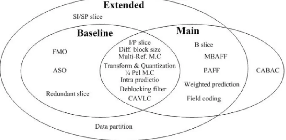
FIG.2-1.SPECIFIC CODING PARTS OF THE THREE PROFILES IN H.264/AVC... 4
FIG.2-2.BLOCK DIAGRAM OF H.264/AVC CODING STRUCTURE... 5
FIG.2-3.BIT-RATE SAVINGS PROVIDED BY CABAC RELATIVE TO CAVLC ... 6
FIG.2-4.EXAMPLE OF THE PROBABILITY MODEL... 7
FIG.2-5.ENCODING PROCEDURE FOR SYMBOL SEQUENCE (C B C E)... 8
FIG.2-6.EXAMPLE OF ARITHMETIC DECODING PROCESS... 9
FIG.2-7.DEFINITION OF MPS AND LPS... 10
FIG.2-8.ENCODING PROCESS OF SUB-DIVIDED INTERVAL MPS AND LPS ... 11
FIG.2-9.EXAMPLE OF ENCODING BINARY ARITHMETIC CODING WITH ADAPTIVE PROBABILITY... 12
FIG.2-10.DECODING OF SUBDIVISION OF MPS AND LPS ... 13
FIG.2-11.CABAD BLOCK DIAGRAM... 14
FIG.2-12.DECODING FLOW OF THE DECISION MODE... 16
FIG.2-13.DECODING FLOW OF THE BYPASS MODE... 17
FIG.2-14.DECODING FLOW OF THE TERMINAL MODE... 18
FIG.2-15.FLOWCHART OF RENORMALIZATION... 19
FIG.2-16.PSEUDO CODE OF THE SUFFIX PART ALGORITHM... 22
FIG.2-17.ILLUSTRATION OF THE NEIGHBOR LOCATION IN MACROBLOCK LEVEL... 27
FIG.2-18.ILLUSTRATION OF THE NEIGHBOR LOCATION IN SUB-MACROBLOCK LEVEL... 27
FIG.2-19.(A) ZIG-ZAG SCAN AND (B) FIELD SCAN... 31
FIG.3-1.BLOCK DIAGRAM OF CABAD ... 34
FIG.3-2.ELEMENTARY OPERATIONS OF CABAD... 35
FIG.3-3.OVERVIEW OF OUR ARCHITECTURE... 36
FIG.3-4.DECODING FLOW AT SYNTAX ELEMENT LEVEL... 38
FIG.3-5.BAD FOR ONE-SYMBOL ARCHITECTURE... 41
FIG.3-6.SIMPLIFY ONE-SYMBOL BAD ARCHITECTURE AND ITS SIMPLY DRAWING... 43
FIG.3-7.CASCADE ARCHITECTURE OF THREE-SYMBOL BAD ... 44
FIG.3-8.EXAMPLE OF TWO-SYMBOL EXPANDING BAD ARCHITECTURE... 45
FIG.3-9.ORGANIZATION OF THE MULTI-SYMBOL BAD ... 48
FIG.4-6.FLOW DIAGRAM OF THE SIGNIFICANCE MAP... 60
FIG.4-7.DECODING ORDER OF SIG._COEFF_FLAG AND LAST_SIG._COEFF_FLAG... 60
FIG.4-8.TIMING DIAGRAM FOR THE ORIGINAL ORGANIZATION OF CONTEXT MEMORY... 61
FIG.4-9.(A)ORIGINAL MODIFIED ORGANIZATION.(B)OUR PROPOSED ORGANIZATION... 61
FIG.4-10.FORMULA OF INTRA PREDICTION MODES... 62
FIG.4-11.MEMORY REARRANGE FOR INTRA CONTEXT MEMORY... 62
FIG.4-12.FULL-VIEW ORGANIZATION OF OUR PROPOSED CONTEXT MEMORY... 63
Chapter 1
Introduction
1.1 Motivation
H.264/AVC is a new international video coding standard developed by the Joint Video Team of ISO/IEC Moving Picture Experts Group and ITU-T Video Coding Experts Group. The new standard can save the bit-rate up to 50% compared to the previous video standard under the same video quality. It employs various advanced coding tools such as multiple reference frame, variable block size, in-loop de-blocking filter, quarter-sample interpolation, and context-based adaptive binary arithmetic coding. Because of its outstanding performance in quality and compression gain, the more and more consumer application products adopt H.264/AVC as its video standard, such as portable video device, video telephony, digital camera …etc.
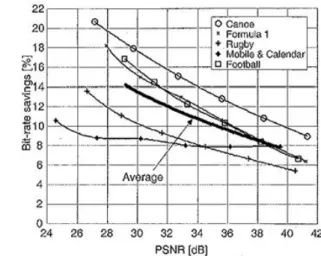
H.264/AVC contains two entropy coding schemes which are context-based adaptive variable length coding (CAVLC) and context-based adaptive binary arithmetic coding (CABAC). Compared to CAVLC, CABAC averagely can save 9%-14% of bit-rate at the expense of higher computation complexity. Therefore, the acceleration of the CABAC
structure efficiently increases the throughput of arithmetic coding. 2) Rearrangement of the context table and using small cache registers improve pipeline hazards.
1.2 Thesis organization
This thesis is organized as follows. In Chapter 2, we present the overview of CABAD for H.264/AVC. We will describe several parts in the chapter such as H.264/AVC standard, arithmetic coding, binary arithmetic coding, binarization decoding flow and context model organization. Chapter 3 shows the proposed architecture of our multi-symbol CABAD design. We focus on M-cascade structure of binary arithmetic decoding engine to promote the throughput. Chapter 4 presents our context memory model and the rearrangement of memory table. The simulation result and implementation is shown in Chapter 5. And we make a brief conclusion and future work in Chapter 6.
Chapter 2
Overview of CABAD for H.264/AVC
H.264 has been developed jointly by ITU-T VCEG and ISO/IEC MPEG. Its data compression efficiency is four and two times better than earlier video standards, MPEG-2 and MPEG-4 respectively. This is due to that H.264/AVC adopts many complicated and computational video coding tools, so it can maintain the video quality as well enhance the coding efficiency. In this chapter, we show the algorithm of CABAD. The CABAD is composed of the arithmetic decoding process, the binarization and the context model. The arithmetic decoding process reads the bit-streams and computes the bin to offer the binarization process for decoding the suitable syntax elements. The context model records the historical probability.
This chapter is organized as follows. In section 2.1, we roughly describe H.264/AVC standard [1]. In section 2.2, the more detail of the binary arithmetic coding algorithm will be shown. In section 2.3, we introduce the algorithm CABAD in H.264/AVC. It contains three modes of decoding process and the renormalization process. In section 2.4, we introduce all kinds of the binarization process. Last we show how to get the neighbor syntax element to index the suitable context model allocation and present the context model related with each syntax element in section 2.5.
2.1 Overview of H.264/AVC standard
H.264/AVC has following advanced features to improve the coding efficiency and video quality, variable block-size motion compensation, quarter-sample-accurate motion compensation, multiple reference picture motion compensation, in-loop de-blocking filter, small block-size transform, arithmetic entropy coding, and context-adaptive entropy coding. Figure 2-1 shows the three profiles of H.264/AVC standard. These three profiles are basic profiles of H.264/AVC. Baseline profile targets applications of low bit rates such as video telephony, video conferencing and multimedia communication because of its low computation complexity; main profile supports the mainstream consumer for applications of broadcast system and storage devices; extended profile is intended as the streaming video profile with error resilient tools for data loss robustness and server stream switching. However, in those profiles small size of blocks and fixed quantization matrix can’t totally hold the image information in high frequency, so H.264/AVC adds Fidelity Range Extensions which contains high profile, high 10 profile, high 4:2:2 profile and high 4:4:4 profile based on main profile for high definition multimedia applications.
Figure 2-2 Block diagram of H.264/AVC coding structure
Figure 2-2 shows the block diagram of the basic coding flow. When doing encoder one frame is inputted, the encoder will do prediction and choose intra or inter prediction according to the input frame type. After the prediction, the original input will subtract the predicted result to get the residual data. Then the residual data will experience discrete-time cosine transform (DCT) and quantization. Finally, entropy coding will encode the DCT coefficients to bit-stream and send it out. In H.264/AVC decoder, the input bit-stream is firstly decoded by entropy decoder and the outputs of the entropy decoder is DCT coefficients, Through de-quantization and inverse DCT, we can fetch the
exp-Golomb codeword tables for all syntax elements except the quantized transform coefficients. For transmitting the quantized transform coefficients, a more efficient method CAVLC is employed. Another method of entropy coding is context-adaptive binary arithmetic coding (CABAC) which can be used in place of UVLC and CAVLC. Compared to CAVLC, CABAC averagely can save 9% to 14% of bit rate at the similar quality from [3], as shown in Figure 2-3. Therefore, we will further discuss CABAC in the following sections.
Figure 2-3 Bit-rate savings provided by CABAC relative to CAVLC
2.2 Algorithm of binary arithmetic coding
2.2.1 Arithmetic coding
Arithmetic coding is a variable-length coding technique. It provides a practical alternative to Huffman coding that can more closely approach theoretical maximum compression ratios. Arithmetic encoder converts a sequence of data symbols into a single fractional number and can approach the optimal fractional number of bits required to
represent each symbol. A scheme using an integral number of bits for each data symbol is unlikely to come so close to the optimum bits. In general, arithmetic coding offers superior efficiency and more flexibility compared to the Huffman coding.
With arithmetic coding, an entire word or message is coded as one single number in the range of [0, 1). This range is divided into sub ranges and assigned to every symbol a range in this line based on its probability, the higher the probability, the higher range which assigns to it. Once we have defined the ranges and the probability line, start to encode symbols, and every symbol defines where the output floating point number lands. We will describe it with an example as follows. First, we consider a 5-symbol alphabet S= {a, b, c, d, e} and their probabilities as shown in Figure 2-4. Each symbol is assigned a sub-range within the range 0.0 to 1.0, depending on its probability of occurrence. In this example, “a” has a probability of 0.1 and is given the range 0~0.1. “b” has a probability of 0.2 and is given the next 20% of the total range, i.e. the range 0.1~0.3. After assigning a sub-range to each symbol, the total range 0~1.0 has been divided amongst the data symbol according to their probabilities.
We would like to encode a message of symbol sequence (c b c e) using the above fixed model of probability estimates. As each symbol in the message is processed, the range is narrowed down by the encoder as explained in the algorithm. Since the first symbol of the message is “c”, the range is first narrowed down to [0.3, 0.7). Then the range is survived to [0.34, 0.42), because it belongs to symbol “b”. According to arithmetic encoding algorithm the last symbol is “c” and hence we could send any number in the range 0.3928 to 0.396. The decoding processing is using the same probability model and will get the same result.
As shown in Figure 2-5, arithmetic encoding calls for generation of a number that falls within the range [Low, High). The below algorithm will ensure that the shortest binary codeword is found. Then we know the number 0.394 is transmitted. 0.394 can be represented as a fixed-point fractional number using nine bits, so our message of symbol sequence (c b c e) is compressed to a nine-bit quantity.
When doing decoding procedure, we find the sub-range in which the received number falls. We can immediately decode that the first symbol is “c” because the number 0.394 belongs to the range [0.3, 0.7). Then the range is narrowed down to [0.3, 0.7) and decoder subdivides this range. We see that the value of 0.394 now falls in the range [0.34, 0.42), so the second letter must be “b”. This kind of process is repeated until the entire sequence (c b c e) is decoded. Following is the algorithm of the arithmetic decoding procedure.
2.2.2 Binary arithmetic coding
This section introduces the basic arithmetic algorithm to understand the binary arithmetic coding algorithm and know how to encode and decode the bit-stream. Arithmetic coding is quite slow in general because we need a series of decision and multiplications. The complexity is greatly reduced if we have only two symbols. According to the probability, the binary arithmetic coding defines two sub-intervals in the current range. The two sub-intervals are named as MPS (Most Probable Symbol) and LPS (Least Probable Symbol). Figure 2-7 shows the definition of the sub-intervals. The lower part is MPS and the upper one is LPS. The range value of MPS is defined as rMPS and the range value of LPS is defined as rLPS, and they are defined as follows. The summation of ρMPS andρLPS is equal to one because the probability of the current interval is one.
Figure 2-7 Definition of MPS and LPS
Depending on the bin decision, it identifies as either MPS or LPS. Assume the bin value of MPS is 1 and the bin value of LPS is 0. If bin is equal to “1”, the next interval belongs to MPS. Figure 2-8(a) shows the MPS sub-interval condition and the lower part of the current interval is the next one. The range of the next interval is re-defined as rMPS. By the way, if we want to achieve the adaptive binary arithmetic coding, the ρMPS is increased to update the probability. On the contrary, the next current interval belongs to
LPS when bin is equal to “0”. Figure 2-8(b) shows the LPS sub-interval condition and the upper part of the current interval is the next one. The range of the next interval is re-defined as rLPS and ρMPS is decreased. The codIOffset is allocated at the intersection between the current MPS and LPS range. Depending on the codIOffset, the arithmetic encoder produces the bit-stream in order to achieve the compression effect.
Table 2-1 Results of encoding process
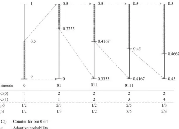
Figure 2-9 Example of encoding binary arithmetic coding with adaptive probability
An example of encoding a binary sequence: 01111, as shown above. Initially the counter is set 1, so the probability is half-and-half. After encoding the bin “0”, the counter of bin “0” increase one so that the probability is adaptively changed. The probability for bin “0” and bin “1” is 2/3 and 1/3 respectively. The procedure is continuous as the pattern. Finally we encode 0.4667 to binary output.
In the binary arithmetic decoder, it decompresses the bit-stream to the bin value which offers the binarization to restore the syntax elements. The decoding process is similar to the encoding one. Both of them are executed by means of the recursive interval subdivision. Something different is described as follows.
It is needed to define the initial range and the MPS probability when starting the binary arithmetic decode. The value of codIOffset is composed of the bit-stream con compared with rMPS. Figure 2-10 illustrates the decoding subdivision of MPS and LPS
condition. If codIOffset is less than rMPS, the condition belongs to MPS. The range of the next interval is equal to rMPS and the probability of MPS is increased. The bin value outputs “1”. The next value of codIOffset remains the current one. If codIOffset is greater than or equal to rMPS, the next interval turns into LPS. The range of the next interval is defined as rLPS and the probability of MPS is decreased. The bin value outputs “0”. The next value of codIOffset is to subtract the rMPS from the current codIOffset.
Table 2-2 Results of decoding process and its comparator
2.3 Algorithm of CABAD for H.264/AVC
2.3.1 System level of CABAD
The main profile uses a more complex entropy coding scheme CABAC which is based on arithmetic coding. In section 2.2.3, we introduce the basic algorithm of the binary arithmetic coding. Although it can achieve the high compression gain, the hardware complexity becomes the problem. In Figure 2-7, it has to compute the value of rMPS and rLPS with two multipliers and processes the next value of codIOffset, range, and the probability by means of the floating adders and comparators. It consumes the lots of hardware cost. According to H.264/AVC standard, it adopts table-base method to decrease the complexity hardware cost. And we will describe that later.
Figure 2-11 CABAD block diagram
First, Figure 2-11 shows the CABAD block diagram consisted of three blocks. 1. Binarization
2. Context Model
3. Binary Arithmetic Decoder
and the BAD has three different modes. In encoder, a given non-binary valued syntax element (e.g. a transform coefficient or motion vector or any symbol with more than 2 values) is uniquely mapped to a binary sequence (called bin-string) by the binarization. On the contrary, in decoder, the binarization process reads the bin string and decodes to the syntax element (SE) by five kinds of decoding ways which will be shown in section 2.4. Last the context model is about the table-based probability.
2.3.2 Three modes of decoding process in CABAD
CABAD offers a far more efficient form of run-length coding by exploiting correlation between symbols. In order to improve the coding efficiency, there are three modes of the binary arithmetic decoders in H.264/AVC system such as the decision mode, bypass mode, and terminal mode. The decision mode includes the utilization of adaptive probability models and interval maintainer, the bypass mode codes for a fast encoding of symbols which are approximately uniform probability, and the last mode of terminal mode is a special fixed executing before end of coding with non-adapting probability state. We will show whole algorithms as follows.
The first algorithm is the decision mode which is shown in Figure 2-12. There are two main factors to dominate the hardware efficiency. One is the multiplier of (range)x(ρMPS )
and the other is the probability calculation. According to H.264/AVC standard, the table-based method is used in place of the multiplication operation. In the decoding flow of the decision mode, codIRangeLPS looks up the table depending on two indexes such as pStateIdx and qCodIRangeIdx. pStateIdx is defined as the probability of MPS which gets from the context model. qCodIRangeIdx is the quantized value of the current range (codIRange). The second factor of the improved method is about the probability calculation to estimate the value of ρMPS. In section 2.2.3, we know that the value of ρMPS
is increased when MPS condition happened and is decreased when LPS condition happened. In Figure 2-12, it shows the table-based method to process the probability estimation. It divides into two parts such as MPS and LPS conditions. It computes the next probability by the transIdxLPS table when the LPS condition happened and by the transIdxMPS table when the MPS condition happened. The two probability tables are approximated by sixty-four quantized values indexed by the probability of the current interval.
The second algorithm is the bypass mode which is applied by the specified syntax element such as mvd and coeff_abs_level_minus1. Figure 2-13 shows the flowchart of the bypass decoding mode. This mode is unnecessary to refer to the context model, and it doesn’t do the probability computation to estimate the probability of the next interval. The computed codIRange doesn’t change which means that it doesn’t do renormalization in the bypass mode.
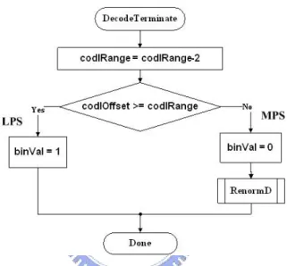
Figure 2-14 Decoding flow of the terminal mode
The third algorithm is the terminal mode. Figure 2-14 shows the decoding flowchart of the terminal mode. The terminal decoding mode is quite simple, and it also doesn’t need the context model to refer to the probability. The value of the next codIRange is always to subtract two from the current codIRange depending on whether the condition belongs to MPS or LPS. The final values of codIRange and codIOffset are required to renormalize when MPS condition happened. The process of the terminal mode is used to trace if the current slice is ended. It occurs one time per macroblock process which is seldom used during all decoding processes.
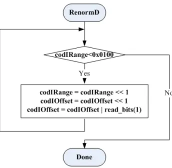
Figure 2-15 Flowchart of renormalization
In the basic binary arithmetic decoder described in section 2.2.3, the floating-point operation is used. That will increase the complexity of the circuit in practical implementation. In H.264/AVC, CABAD adopts the integer operation to improve. We do the renormalization to keep the scales of codIRange and codIOffset. Figure 2-15 shows the flowchart of renormalization. The MSB of codIRange always keeps logic one in order to realize the integer operation. If the MSB of codIRange is equal to logic zero, the value of codIRange has to be shifted left until the MSB of codIRange is equal to one. Depending on the shifted number of codIRange, codIOffset fills the bit-stream in LSB.
Fixed-length binarization (FL) process Special binarization process
This section is organized as follows. In section 2.4.1, the decoding flow of the unary code is shown first. The unary code is the basic coding method. Section 2.4.2 shows the truncated unary code which is the advanced unary coding. It is applied in order to save the unary bit to express the current value. Section 2.4.3 is the Exp-Golomb binarization process. The UEGk is only used for the residual data and the motion vector difference (mvd). In section 2.4.4, we describe the fixed-length decoding flow. It is the typical binary integer method. And section 2.4.5 is the special definition by means of the table-base method.
2.4.1 Unary (U) binarization process
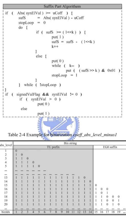
Table 2-3 is the unary code of binarization process. The bin string of a syntax element having (unsigned integer) value synElVal which is a bin string of length synElVal + 1. The bin string index is defined as binIdx. The bins for binIdx less than synElVal are equal to logic one. The bin with binIdx equal to synElVal is equal to logic 0. So the number of logic one is equal to synElVal.
2.4.2 Truncated unary (TU) binarization process
The truncated unary binarization is based on the unary binarization and has an additional factor of cMax which is defined as the maximum length of the current bin string. When the value of syntax element (synElVal) is less than cMax, the U binarization process is invoked. If synElVal is equal to cMax, the bin string is a bit string of length cMax with all bins being equal to logic one. For example, it is assumed that synElVal equals to 4. If the value of cMax is “5”, the result of bin string is equal to “11110”. If the value of cMax is “4”, the result of bin string is equal to “1111” where the end bit of “0” is truncated in this case.
2.4.3 Unary/k-th order Exp-Golomb (UEGk)
binarization process
The UEGk code is composed of two parts which are the prefix and suffix bit string. The prefix part of UEGk is specified by using the TU binarization process for the prefix part min( uCoff, Abs(synElVal) ) of a syntax element value synElVal with cMax equals to uCoff, where uCoff > 0. So the prefix part is dominated by cMax. Figure 2-16 shows the suffix part algorithm by means of the pseudo code. In the CABAD binarization engine, it
Figure 2-16 Pseudo code of the suffix part algorithm
2.4.4 Fixed-length binarization (FL) process
Table 2-5 Bin string of the FL code
The fixed-length code is represented by means of the typical unsigned integer. For example, the value of “610” is equal to “1102”. The value of decimal type changes to the
binary format, which requires fixed-length code. FL binarization is constructed by using a fixedLength-bit unsigned integer bin string of the syntax element value, where fixedLength = Ceil( Log2 (cMax + 1) ), ( Cei(x) means the smallest integer greater than
or equal to x.). Table 2-5 shows the fixed-length code definition. In this table, the cMax equals seven and the fixedLength will be three. All syntax elements which are decoded by the FL binarization are always represented with three binary bits.
coding flows. In H.264/AVC [1], it adopts the table-based method to define mb_type and sub_mb_type. The binarization engine reads the bin string and checks if the bin string is mapped the specified location in these tables. If the bin string is found in these tables, it can look up the current macroblock type.
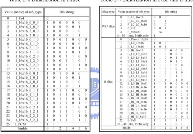
Table 2-6 Binarization in I slice Table 2-7 Binarization in P/SP and B slice
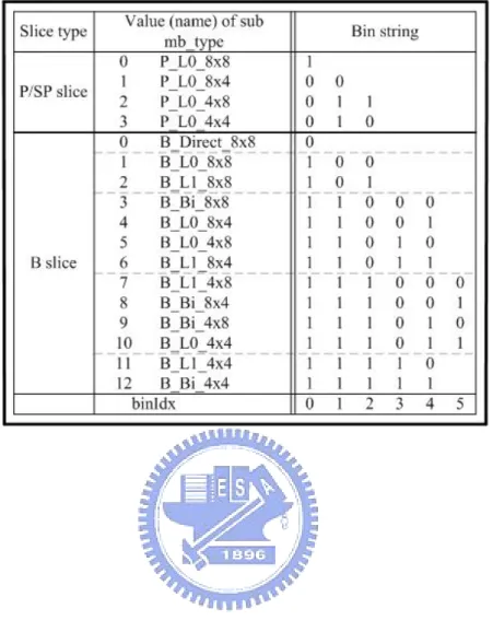
The binarization scheme for coding macroblock type in I slice is specified in Table 2-6. The binarization scheme for P macroblock type in P/SP slice and B macroblock in B slice are specified in Table 2-7. For P/SP and B slices, the specification of the binarization for sub_mb_type is given in Table 2-8.
2.5 Context model organization
The values of the context model offer the probability value of MPS (pStateIdx) and the historical value of bin (valMPS) in order to achieve the adaptive performance. Context provides estimates of conditional probabilities of the coding symbols, and it has to prepare 399 locations of the context model to record all encoding/decoding results. Utilizing suitable context models, given inter-symbol redundancy can be exploited by switching between different probabilities according to coded symbol in the neighborhood of the current symbol.
The context model index is dominated by two factors such as ctxIdxOffset and ctxIdxInc. ctxIdxInc is the only one factor related with the syntax element of the neighbor blocks. The variable syntax elements refer to the left and top block to define the ctxIdxInc of the first binIdx such as mb_type, mb_skip_flag, ref_idx, mb_qp_delta, …, etc. The generic form of the equation is given as follows. The conditional term condTermFlag (A, B) describes the functional relationship between the spatially neighbor block A and B.
In CABAC system, the referred position is based on the current block which can treat as not only the macroblock but also the sub-macroblock. So we have two methods to allocate the required blocks.
Figure 2-17 Illustration of the neighbor location in macroblock level
Figure 2-18 Illustration of the neighbor location in sub-macroblock level
The first method is to get neighbor in macroblock level. Figure 2-17 shows the left (A) and top (B) macroblocks of the current one. And the second method is in sub-macroblock level, as shown in Figure 2-18. The coordinate of the current sub-macroblock is defined as (sub_mb_x, sub_mb_y). If sub_mb_x is not equal to “0”, the left sub_macroblock is in the left side of the current macroblock. If sub_mb_x is equal to “0”, the left
syntax elements of the sub-macroblock 12, 13, 14, 15 also have to be stored in order to record the top sub-macroblock.
2.5.1 Assignment process of context index
H.264/AVC uses the above two rules to allocate the context model. The first rule is used except residual data of syntax element (coded_block_flag, significant_coeff_flag, last_significant_coeff_flag, and coeff_abs_level_minus1). The context model index is equal to the sum of ctxIdxOffset and ctxIdxInc. Depending on the syntax element and the slice type, we can find the value of ctxIdxOffset in Table 2-9. The value of ctxIdxInc is looked up in Table 2-10 by referring to the syntax element and binIdx. In Table 2-10, the word of “Terminal” means that the encoding/decoding flow enters the terminal process. If the generated bin is equal to “1”, the slice has to be stopped and encodes/decodes the next slice.
Table 2-9 Syntax element and associated definition of ctxIdxOffset
Table 2-11 Specification of ctxIdxInc for specific values of ctxIdxOffset and binIdx
For special ctxIdxInc, that is derived by using the value of prior decoded bin value. Table 2-11 shows the value of ctxIdxInc in special binIdx.
The second rule is the context index method for the residual data such as coded_block, significant_coeff_flag, last_significant_coeff_flag, and coeff_abs_level_minus1. The value of the context model index is the sum of ctxIdxOffset, ctxIdxBlockCatOffset, and ctxIdxInc. The assignment of ctxIdxOffset is shown in Table 2-9. The value of ctxIdxBlockCatOffset is defined as Table 2-12 which is dominated by the parameters of syntax element and ctxBlockCat. The ctxBlockCat is the block categories for the different coefficient presentations. ctxBlockCat sorts five block categories in Table2-13. maxNumCoeff means the required coefficient number of the current ctxBlockCat.
For the syntax elements significant_coeff_flag and last_significant_coeff_flag, the value of ctxIdxInc is defined as the scanning position that ranges from 0 to “maxNumCoeff - 2” in Table 2-13. The scanning position of the residual data process has two scanning orders. One is scanned for frame coded blocks with zig-zag scan and the other is scanned for field coded blocks with field scan, as shown in figure 2-19.
Figure 2-19 (a) zig-zag scan and (b) field scan
2.6 Paper survey for CABAD designs
In this section, we will introduce some of CABAD decoding designs which have been published recently (2005 ~ 2007). The main differences of all of these are almost in arithmetic design due to that the arithmetic coder is the main dominator of throughput for the whole CABAD system. The CABAD decoder designs are introduced as follows.
1. For the CABAD design of [4] proposed by Yongseok Yi, In-Cheol Park, the initial design without optimization takes 7.43 clock cycles per bin. The optimization
per bin. But the throughput of this design is not high-product because it is one-symbol architecture and its context memory needs great hardware cost.
2. The high-performance CABAD design is proposed by J. W. Chen, Y. L. Lin [5]. It proposes three parallel processing techniques. The initial design without optimization decodes 0.44 bins per cycle. Three parallel processing techniques are shown as follows.
(1) Parallelizing the tasks of decoding coefficients and getting neighboring data. (2) The two-bin-per-cycle decoding method.
(3) Context table rearrangement method.
After adopting these methods, the throughput is up to 0.99 bins per cycle.
3. The CABAD decoder design of [8] is proposed by Y. C. Yang, C. C. Lin, H. C. Chang et al. They adopt four techniques to improve the performance of CABAD. They are adopting 1) two-symbol architecture pipeline scheduling, 2) using segmented context tables, 3) adding cache registers to store the value of context memory, and 4) doing look-ahead codeword parsing.
4. We also reference the multi-symbol architecture design for arithmetic encoder [6] which is proposed by Y. J. Chen, C. H. Tsai, L. G. Chen. The one-symbol arithmetic coder was partitioned into four stage: Update State, Update Range, Update Low and Output. And then they extend the architecture of one-symbol arithmetic encoder to arbitrary m-symbol.
5. A novel configurable architecture of CABAC encoder [7] is proposed by Y. J. Chen, C. H. Tsai, L. G. Chen. The traditional processing unit is divided into two parts, MPS encoder and LPS encoder. With different arrangements of these two basic components, they develop two types of ML-decomposed structures, such as 1) ML cascade architecture and 2) throughput-selection architecture. ML cascade architecture exploits the complementary critical path of MPS and LPS coder, and
throughput-selection architecture offers more choices of ML cascades to select the highest throughput one.
Chapter 3
Multi-Symbol of Binary Arithmetic
Decoder Engine
3.1 Overview of CABAD system
Figure 3-1 Block diagram of CABAD
Arithmetic coding is a recursive subdivision procedure. It contains two data dependency which results in intensive computation. Firstly, the interval is specified by
range and offset. Depending on symbol is the Most Significant Symbol (MPS) or Least
Significant Symbol (LPS), the next interval is updated as one of two sub-intervals. The second is the adaptive probability state of the context of symbol. The probability table will be updated according to the current symbol. Figure 3-1 is the system architecture of
CABAD which consists of three main modules called the binary arithmetic decoder, the binarization engine, and the context model. The entire decoding procedure is described as follows. When starting to decode, it has to initialize the context model by looking up the initial table. BAD reads bit-stream to get the bin value. At the same time, it refers to the current probability from the context model to find the sub-range of MPS or LPS and updates the probability of the location of the current context model index (ctxIdx). The bin string from several bin values is fed to the binarization engine. Then the binarization engine will send out the value of syntax element. Address Generator generates the address of the context model which has been described in section 2-5. Due to these strict data dependencies, the elementary operations can hardly be processed in parallel.
Figure 3-2 Elementary operations of CABAD
context selection to BAD stage.
Figure 3-3 Overview of our architecture
Figure 3-3 is overview of our architecture. γbase(s) is a base context index generated
from the AG stage as the ctxIdxOffset definition from standard [1]. The set of context memory data Cj(s) in the same syntax element is gotten from context memory according to γbase(s) and stored in a small storage called the context state register (CSR). After the
context memory is obtained, the BAD stage takes place. In our BAD stage, it contains three parts such as context selection, binary arithmetic decoding core, and binarization engine. We select needed context data (c1,c2,…) from Cj(s) according to binIdx
(ctxIdxInc) and feed them to BAD core. At the same time, we should update each of the context data. For example, if ctx1 and ctx2 are the same, the pState and valMPS of ctx2
should be replaced by the updated ones of ctx1. When working BAD core, the symbol is
decided by comparing the coding offset and the coding range. Then the renormalization follows to keep the coding range and the coding offset to a fixed precision. Then, we send
the bin string (b1, b2, b3) to do the binarization and resolve the value of syntax element.
Besides, only the updated values of context data ci corresponding to those valid bins
should be written back to CSR. Finally, the data Cj(s) of CSR will write back to context memory. The part of BAD core is described in next section, and the detail of context model in next chapter.
3.2 Statistics and analysis of syntax elements
Figure 3-4 Decoding flow at syntax element level
Figure 3-4 is the state transition at the syntax element level. H.264/AVC defines twenty-five syntax elements. Many syntax elements only need one bin to decode (like significant_coeff_flag, last_significant_coeff_flag, end_of_slice_flag, coded_block_flag, and intra_pre_mode_flag …. First two of them have around 40% of bins). And others need multiple bins to get its information (like coeff_abs, rem_intra_pre_mode, mb_type, sub_mb_type, ref_idx, mvd …, etc.).
Table 3-1 Percentage of the bins at each syntax element
bin%
syntax element QP36 QP30 QP24 QP18 avg Intra_pred_flag, intra_rem 1.68 3.34 4.01 2.85 2.97 sig. & last_sig. 40.51 40.83 39.05 37.46 39.46 coeff_abs 25.98 31.87 38.12 44.08 35.01 MVD 4.87 5.00 5.23 6.67 5.44 Ref_frame 0.52 0.38 0.29 0.24 0.36 other 26.43 18.57 13.30 8.69 16.75
Table 3-2 Percentage of the cycle counts at each syntax element
cycle%
syntax element QP36 QP30 QP24 QP18 avg Intra_pred_flag, intra_rem 1.86 3.72 4.51 3.26 3.34 sig. & last_sig. 44.78 45.35 43.84 42.77 44.19 coeff_abs 21.12 26.67 32.62 38.47 29.72 MVD 3.91 3.99 4.22 5.52 4.41 Ref_frame 0.58 0.43 0.32 0.28 0.40 other 27.75 19.84 14.49 9.70 17.95
Table 3-1 and Table 3-2 are shown the percentage of decoded bins and cycle counts of different syntax elements. "sig.& last_sig.” and “coeff_abs” have most of decoding bins. Therefore, how to enhance the throughput would be divided into two parts. The first is our multi-symbol architecture that can decode multiple bins per cycle. It is shown in next section. But the multi-symbol architecture will not enhance the performance of the one-bin syntax elements such as sig.& last_sig. Then secondly, we rearrange our context
Table 3-3 Percentage of each concatenate symbol
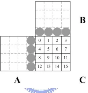
Table 3-3 is the statistics of the average percentage of each symbol alignment. It simulates under executing four CIF sequences (stefan, foreman, news and mobile) by JM8.2. The number of frame is 200 and we set QP16, QP28, and QP40. We find the percentage of concatenate M-symbol is obviously higher than others, especially MMM in 3-symbol and MM in 2-symbol. Take 3-symbol an example, we divide four orders of the happening probability (from most probability to least probability). First group is MMM and it contains 44%. Second group are MML, MLM, and LMM, and they contain 13% respectively. Last group is LLL and it contains 3%. It is efficient that the concatenate symbols (MMM) will be improved firstly.
1. MMM
2. MML, MLM, LMM 3. MLL, LML, LLM 4. LLL
3.3 Proposed multi-symbol architecture
In this section, we extend the architecture of one-symbol arithmetic decoder to three-symbol. It has data dependencies in range and offset. Depending on symbol is the Most Significant Symbol (MPS) or the Least Significant Symbol (LPS), next interval is updated as one of two sub-intervals. The range and offset equations are as follows,
MPS: Rangen = Rangen-1 – rLPSn
Offsetn = Offset n-1
LPS: Rangen = rLPSn
Offsetn = Offset n-1 – Range n-1 + rLPSn
where n represents current symbol and rLPS is the estimated range when coding LPS.
Table 3-4 Results for range, offset and binVal at each mode
The basic Binary Arithmetic Decoding core is as shown in Figure 3-5 [11]. For hardware sharing, it combines three modes (decision, bypass, and terminal) into the architecture, and Table 3-4 shows the results of range, offset, and bin value in each mode. The shaded adder is also the comparator which calculates the temporal variables OffsetX and RangeX, and it will decide the symbol is MPS or LPS resulting in the binVal. The table of rangeLPS has 256 entries. The large table is unfortunately located in the critical path when decoding multi-symbol. To speed up, we divide the table into two parts, 64:1 and 4:1 as like [6]. Then, we can pre-compute the greater parts (64:1) when doing other operations. Table 3-5 shows the dependency of Bin_flag, valMPS, and Bin_value. The result of bin value is Bin_flag depending on valMPS. And the signal Bin_flag is the msb of the result from the subtractor of Offset and RangX. When Offset is less than RangX, the signal of Bin_flag will be set 1. It means that the decoding symbol is MPS, and the decoding Bin value is the function XOR of the two signals Bin_flag and valMPS.
Table 3-5Dependency of symbol, Bin_flag, valMPS and bin value comparator Bin_flag Symbol Bin_flag valMPS Bin value Offset >= RangX 0 LPS 0 0 1
Offset < RangX 1 MPS 1 0 0 0 1 0 1 1 1
3.3.2 Cascaded structure of multi-symbol BAD
The intuitive method for multi-symbol BAD is to cascade one-symbol architecture as shown in Figure 3-6. It doesn’t decode next bin until the result of the comparator of current bin, so that the critical path of the one-symbol architecture will have two adders and the rangeLPS table. If we extend to three-symbol, the critical path is too long that will be six adders and three rangeLPS tables. The hardware cost is three times than one-symbol architecture. Figure 3-7 is simply drawing of the cascade architecture of three-symbol BAD [5].
3.3.3 Extending structure of multi-symbol BAD
Figure 3-8 Example of 2-symbol expanding BAD architecture
As shown in Figure 3-8, if we expand the range and offset equation of two-symbol BAD, the architecture can reduce the long critical path. The following equations are the results of Range and Offset. LPS1 represents that the first decoding symbol is LPS, and
LPS2 represents that the second decoding symbol is LPS, and so forth to MPS1 and MPS2.
LL_R represents the result of range which decodes concatenate symbols of both LPS. The same as to LL_O, and the last letter O represents the result of Offset. And LM_R
When doing the first symbol’s comparator, it also does the second symbol’s operation. In addition, the rangeLPS table can be computed in advance because we already know the next decoded symbol is MPS or LPS. As a result, it can reduce one adder time and one rangeLPS table time if every adding one-symbol extending architecture. So the critical path of the two-symbol extending architecture is three adders and one rangeLPS table.
It is easy to expand to three-symbol architecture, and its critical path is four adders and one rangeLPS table. We reduce the critical path of two adders and two rangeLPS tables compared to the cascade three-symbol BAD architecture. But the hardware cost of extending three-symbol architecture is seven times larger than one-symbol architecture. The hardware cost is too great. Next we propose an efficient method to reduce the critical path and let cost down.
3.3.4 M-cascade of multi-symbol architecture
Table 3-6 Critical path of the adders in three-symbol extending BAD MMM MML MLM MLL Num. of adders time 3 4 3 4
LLL LLM LMM LML Num. of adders time 4 3 2 3
Table 3-6 is shown the critical path of the needed adders of decoding each concatenate symbol case.
The critical path of cascade three-symbol architecture is too long and the hardware cost of extending three-symbol architecture is too large. Case control study with Table 3-6, Table 3-3 and hardware design, in concatenate three symbols we finally choose the decoding process of MMM and MML to make sure hardware sharing (cost down) and efficiently enhance the throughput. We can speed up 57% decoding bin and minimize the hardware cost and the critical path.
Figure 3-9 Organization of the multi-symbol BAD
Table 3-7 Case of multi-symbol which our architecture can decode case
1-symbol L, M 2-symbol ML,MM 3-symbol MML,MMM
We propose our M-cascade of multi-symbol BAD architecture in Figure 3-9 The architecture can decode three concatenate symbol whether it is decision mode or bypass mode, and it only executes the case of symbol alignment(L, M, ML, MM, MML, MMM) as shown in Table 3-7. The architecture decodes next symbol when the prior symbol is
M-symbol, so we call it M-cascade architecture. For an example, if we want to decode the symbol streams MLLMMM, our architecture will decode ML firstly and L at next cycle, and decode MMM finally. So it doesn’t always execute up to three symbols. First problem is that the architecture of other symbol alignment (MLM, MLL, LMM, LML, LLM, and LLL) doesn’t parallel processing in our design. These symbol alignments should be separated to one-symbol and two-symbol or three one-symbols. Because we focus on the improvement of the most percentage, we choose the case of MMM and the case of MML to decoding. Secondly, the binarization engine judges the three bin string if the bin values are the valid symbols. The signal binvalidx_BAD is to discriminate the correctness of the decoded bin value by our confining architecture (only decoding L, M, ML, MM, MML, MMM). Table 3-8 is shown their relation. Then we sent those needed signal to execute the binarization. If the first n bins are valid, the n-th results of codIOffset and codIRange have to be selected by the binarization engine to offer the next BAD.
In Figure 3.9, bit stream buffer is fed to ○1 , ○2 , ○3 , ○4 , ○5 and Renormalization
unit. ○1 , ○3 and ○5 is about bypass decoding process. ○2 is the operation of the
renormalization after decoding “M”, and ○4 is after decoding “MM”.
Table 3-8 Truth table of binvalid?_BAD related to our BAD architecture INPUT OUTPUT
MSB_1 MSB_2 MSB_3 binvalid1_BAD binvalid2_BAD binvalid3_BAD
3.4 Pipeline organization
The most effective way to enhance the performance is to exploit the pipelining scheme. In decision mode, it takes 4 cycles to complete one bin coding in conventional processing without pipelining. The bypass mode and the terminal mode doesn’t need the probability data, so it will not execute the part of context memory and takes one cycle to complete one bin coding, as shown in Figure 3-3. We show these stages to schedule the pipeline organization in this section. And we also show some restricts in our design.
Figure 3-10 Timing diagram of the pipeline comparison
Figure 3-10 shows the timing diagram of the pipeline comparison for decision mode, and it is almost the same as [4]. But we move the CS operation to BAD stage.
In conventional scheme, it must compute context address every symbol processing and load context data (pState and valMPS) to next stage without CSR. In our design, we load a series set of context data to CSR in syntax element beginning and write back to
context memory in syntax element end. We only read and write context memory one time in every syntax element (except the two syntax element of significant_coeff_flag and last_significant_coeff_flag), but in conventional scheme it will read and write context memory more times depending on how many the decoded bins in that syntax element. It can be found that the conventional scheme produces one bin every 4 cycles in average, and the other one with pipelining and CSR produces 1~3 bins every cycle. Compared with the conventional organization, the proposed design with the pipeline can save large the process cycles. Next we show the timing diagram of some restricts and situation resulted from our multi-symbol BAD unit.
Our architecture doesn’t support the concatenate symbol MLM, but support ML. It will judge the symbol M of binIdx = 5 is invalid, and forward the value of binIdx = 4. Although the comparator decide the decoding symbol of binIdx = 5 is M, and it is indeed, but the output of codIRange and codIOffset will be wrong. That will result in the wrong following process. So we put some logic to estimate.
Figure 3-11(b) is the timing diagram happening when syntax element change. When a new syntax element is to be decoded, the pipeline is stalled for two cycles to update and load the series set of context data. The CSR (Figure 3-3) will write back the context data of prior syntax element to context memory and then load the new one of current syntax element. When the correct output of ML is decoded and sent to the binarization engine, the binarization judges it’s the end of syntax element. Then we write back the CSR to context memory, and at next cycle we will load context data of new syntax element to CSR. It wastes two cycles and it is also the bottleneck of our architecture.
When decoding the syntax element of MVD and coeff_abs, it may decode the bin using bypass mode or decision mode. This part is shown the schedule of the decision mode changing to the bypass mode in our architecture. When the decoding bins in these two syntax elements are more than the value boundary (£), the following bins will use bypass mode to decode. The value boundary (£) of MVD and coeff_abs is set 8 and 13 respectively as shown in Table 3-9.
Table 3-9 The parameters of the decision mode changing to the bypass mode Syntax element Value boundary Should decode more bins using bypass mode
MVD 8 n+2
coeff_abs 13 N
is 0, it should decode n+2 bins using bypass mode in following process. The situation is also the same in syntax element coeff_abs. If the decoding bins are more n than 13 until the decoding bin value is 0 in syntax element coeff_abs, it should decode n bins using bypass mode in following process. And both of them, the last decoding bypass bin is also the sign bin. If decoding bins in the two syntax element are less than the value 8 and 13 respectively until the decoding bin value is 0, it should decode more one bin by bypass mode as sign bin. And the changing to bypass mode, it always happens at next cycle whether the concatenate symbols which our architecture can support or not. Figure 3-12 is an example of syntax element MVD.
syntax element MVD. When binIdx = 6 decoding the result of bin value = 0, it decodes more one bin at binIdx = 7 as sign bin at next cycle. Then this syntax element process finish. Figure 3-12(b) is the situation of the decoded bins more than 8 until bin value = 0. When binIdx = 10 decoding the result of bin value = 0, we will know the result of binIdx = 11 is wrong although the concatenate symbols MML our architecture can support. Besides we should decode more 5 bins using bypass mode at next follows cycles.
Chapter 4
Structure of Context Model
4.1 Overview of the context model
The values of the context model depending on the context index (ctxIdx) offer the probability value (pStateIdx) and the historical value of bin (valMPS) in order to achieve the adaptive performance. We have to prepare the 399 locations of the context model to record all decoding results. And two kinds of context model index methods allocate the context model.
ctxIdx = ctxIdxOffset + ctxIdxInc
Figure 4-1 is the traditional organization of context memory, it is dependent on syntax element and the slice type as shown in Table 2-9. The context memory in traditional organization needs 399x7 bits.
In our multi-symbol design, context model must provide multiple context values and set these values to corresponding BAD operations. In context memory load stage, we load a series set of context data (Cj(s)) to CSR according to the context base γbase(s) [4]. Theγbase(s) is the ctxIdxOffset or the sum of ctxIdxOffset and ctxIdxBlockCatOffset respectively to the two equations, as follows.
Figure 4-2 Structure of CSR
CSR architecture is shown in Figure 4-2. The difference from [4] is that the structure of CSR has ten registers to hold the context data from the read subset Cj(s). Since the
range of context index increments lies in [0, 9] for the syntax element coeff_abs_level, we set the register file to 10.
After loading the subset of context elements to CSR, we must choose the correct three set of context data (pState and valMPS) to the BAD unit. The problem is that some ctxIdxInc of syntax element need look for bin value (as shown in Table 2-11) and use the adaptive probability table. Context selection calculates the index to achieve by using the lookup logic and exploiting the current valMPS, so that the problem of ctxIdxInc can be resolved. Because of our multi-symbol M-cascade archticture, we use the characteristic to combine the data dependency of valMPS and lookup logic to get each ctxIdxInc, so that we can get the correct context data (pState and valMPS). Then if ctx1 equals to ctx2, the pState of ctx2 should be replaced by the updated one of ctx1. Finally the updated values of context data should be written back to CSR. Figure 4-5 is the part of our context selection.
4.2 Context memory
To load the ten context elements at once, we need a 70-bit-wide memory configuration. Figure 4-3 [4] shows the context memory organization that is optimal in the sense of memory size required when using our architecture, and that needs 400x7 bits. But in this arrangement, some syntax elements will take more cycles to complete read/write the full context data of the decoding bins iteratively. We modify the optimal organization to read all the elements of each subset in one cycle, as shown in Figure 4-4 [4]. But the modified organization lets memory increase to 670x7 bits. In next section, we propose the new modified context memory. It will decrease the memory size to 550x7 bits and simultaneously enhance the throughput.
Figure 4-5 Modified data arrangement of context memory
4.2.1 Memory rearrangement
In this section, we proposed a new context memory. It not only decreases the memory size but also enhance the throughput of CABAD. According to analysis shown in Table
parts. Figure 4-6 is the flow diagram of the significant map and Figure 4-7 shows an example of the decoding order of significant_coeff_flag and Last_significant_coeff_flag. For each coefficient in scanning order, a one-bit symbol significant_coeff_flag is transmitted. If the bin value of the significant_coeff_flag symbol is 1 at this scanning position, a further one-bit symbol last_significant_coeff_flag is processing. This symbol indicates if the current significant coefficient is the last one inside the block or if the further coefficients follow.
Figure 4-6 Flow diagram of the significance map
Figure 4-7 Decoding order of sig._coeff_flag and last_sig._coeff_flag
As the decoding order, the change of the syntax element is too frequent (sig._coeff_flag → last_sig._coeff_flag or last_sig._coeff_flag → sig._coeff_flag). It will decrease the performance of multi-symbol CABAD because our architecture with the context memory organization (as shown in Figure 4-8) stall two cycles to change the
syntax element. Our design can concurrently read a series subset of two context data of sig._coeff_falg and last_sig._coeff_flag pair from context memory. Figure 4-9(a) is the original part organization of context memory of sig._coeff_flag and last_sig._coeff_flag, and Figure 4-8 its timing diagram. Figure 4-9(b) is our proposed organization which can read/write five pairs in one memory access to decrease the frequency of memory access and promote the decoding bins of this syntax element per cycle to two bins, originally decoding one bin. We can decrease the size of memory about significance map from 360x7 bits to 260x7 bits. Besides, we can save the two stalls.
Decoding the iteration of prev_intra4x4_pre_mode_flag and rem_intra4x4_pre_mode, we finally decode the syntax element intra_chroma_pred_mode, as shown the formula in Figure 4-10. And Figure 4-11 is the part of memory rearrange of intra memory. We can decrease the size of memory about intra syntax from 30x7 bits to 10x7 bits.
Figure 4-10 The formula of intra prediction modes
Figure 4-12 Full-view organization of our proposed context memory
Figure 4-12 is our last context memory organization which is combined above technique. Its location at memory address corresponding to the syntax element and the ctxIdxOffset defined by standard.
Chapter 5
Simulation and Implement Result
5.1 Simulation result
5.1.1 Performance in each syntax element
Table 5-1 Performance of bin/cycle in each syntax element by different QP bin/cycle
syntax element QP36 QP30 QP24 QP18 avg Intra_pred_flag, intra_rem 1.78 1.60 1.44 1.38 1.55 sig. & last_sig. 1.07 1.08 1.08 1.09 1.08 coeff_abs 0.90 1.01 1.12 1.27 1.08 MVD 1.02 1.16 1.22 1.22 1.16 Ref_frame 1.06 1.06 1.06 1.06 1.06 other 0.63 0.62 0.64 0.68 0.64
Table 5-1 is the performance of bin per cycle in each syntax element. Our multi-symbol architecture can enhance more than one bin per cycle in the syntax elements which need concatenate symbol, i.e. coeff_abs, MVD, and Ref_frame etc. And intra related syntax element and significance map also can up to one bin per cycle because of our context memory rearrangement. We successfully achieve decoding multiple symbols per cycle to enhance the performance of the throughput.
5.1.2 Performance of our proposed design
In this section, first we compare the performance of our architecture with a conventional implementation which does not exploit the proposed schemes, that is, one symbol architecture and the elementary operations as shown in Figure 3-2 are not pipelined and the memory organization of Figure 4-1 is used. Table 5-2 summarizes the decoding performance of our architecture and the column of Test sequence I, P, B means I slice, P slice and B slice respectively. The column of Decoded Bins and Total cycles show the number of symbols and the number of decoding cycles. Test sequences adopt 1080HD (1920x1088) which are sunflower, station and riverbed. All the sequences are encoded by reference software JM8.2 in Main Profile at Level 4.0. Sequence type is IBBP and IntraPeriod is set 10. Total encoded frames are 240 and the frame rate is 30fps.
As shown in Table 5-2, in different QP(36, 30, 24, 18) the uses of our architecture result in almost 3.5 times speedup throughput on the average compared to the conventional architecture. The number of Total cycles exclude the time for the RISC to process parameter set and slice headers, the context memory initialization time for each slices, and the macroblock initialization time. So the Total cycles means processing arithmetic coding and read/write context memory.
Table 5-2(a) Improvement of decoding performance in QP36
IBBP - QP36 Conventional Scheme Proposed Design
PSNR
Bit-Rate (Mbps)
Test Sequence Decoded Bins Total cycles cycle/MB cycle/bin Total cycles cycle/MB cycle/bin
Total 159753127 580824325 299.07 3.636 176556185 90.91 1.105 I 5336516 19208945 294.25 3.600 6038969 92.51 1.132 P 53991759 193977177 330.16 3.593 59013412 100.44 1.093 35.93 10.814 sunflower B 100424852 367638203 285.15 3.661 111503804 86.49 1.110 Total 98680596 357874098 184.27 3.627 120002067 61.79 1.216 I 3856447 13922923 213.28 3.610 4605947 70.56 1.194 P 35125766 126904661 216.00 3.613 42158820 71.76 1.200 35.46 6.869 station B 59698383 217046514 168.35 3.636 73237300 56.80 1.227 Total 187244878 672465916 346.26 3.591 206312056 106.23 1.102 I 5529299 20013020 306.57 3.619 6445327 98.73 1.166 P 56066623 201661669 343.24 3.597 62587331 106.53 1.116 1080p 34.26 13.896 riverbed B 125648956 450791227 349.65 3.588 137279398 106.48 1.093 Average 35.22 10.526 148559533.7 537054779.7 276.54 3.618 167623436 86.31 1.141
Table 5-2(b) Improvement of decoding performance in QP30
IBBP - QP30 Conventional Scheme Proposed Design
PSNR
Bit-Rate (Mbps)
Test Sequence Decoded Bins Total cycles cycle/MB cycle/bin Total cycles cycle/MB cycle/bin
Total 262367865 948899829 488.60 3.617 265943740 136.94 1.014 I 9362625 33804366 517.84 3.611 10113758 154.93 1.080 P 92034331 329060572 560.08 3.575 93605849 159.32 1.017 39.25 19.736 sunflower B 160970909 586034891 454.54 3.641 162224133 125.83 1.008 Total 194248697 701241503 361.08 3.610 213932462 110.16 1.101 I 7771132 28040647 429.54 3.608 8742360 133.92 1.125 P 67533891 242356782 412.51 3.589 74942632 127.56 1.110 38.27 15.407 station B 118943674 430844074 334.17 3.622 130247470 101.02 1.095 Total 325432948 1163550682 599.13 3.575 339055561 174.58 1.042 I 10294589 37282526 571.12 3.622 11480410 175.86 1.115 P 93733898 336605180 572.93 3.591 100792285 171.56 1.075 1080p 37.3 27.399 riverbed B 221404461 789662976 612.48 3.567 226782866 175.90 1.024 Average 38.27 20.847 260683170 937897338 482.93 3.601 272977254.3 140.56 1.052