模糊細胞神經網路整合系統

全文

(1)國立交通大學電機與控制工程學系博士論文. 模糊細胞神經網路整合系統 A Fuzzy Cellular Neural Network Integrated System. 研究生：張俊隆指導教授：林進燈. 中華民國九十五年一月. i.

(2) 模糊細胞神經網路整合系統 A Fuzzy Cellular Neural Network Integrated System 研究生：張俊隆. Student：Chun-Lung Chang. 指導教授：林進燈博士. Advisor：Dr. Chin-Teng Lin. 國立交通大學電機與控制工程學系博士論文 A Dissertation Submitted to Department of Electrical and Control Engineering College of Electrical Engineering and Computer Science National Chiao Tung University in partial Fulfillment of the Requirements for the Degree of Doctor of Philosophy in Electrical and Control Engineering January 2006 Hsinchu, Taiwan, Republic of China. 中華民國九十五年一月. ii.

(3) 模糊細胞神經網路整合系統. 摘要. 無論從應用或生物觀點，使用一組平行的細胞神經網路(cellular neural networks, CNN)以完成高階資訊處理與推論能力已被廣泛的接受。如此的整合型細胞神經網路可以解決比較複雜的問題。本論文提出一種以遞迴式模糊神經網路（recurrent fuzzy neural network）的架構以自動建構CNN整合系統。這個稱為 RFCNN/RFCCNN (recurrent fuzzy CNN/ recurrent fuzzy coupled CNN)的整合系統可以同時自動的學習CNN的網路結構與參數。其網路結構學習包括模糊規則（fuzzy rules）與CNN數目的建立；其參數學習包括模糊歸屬函數與CNN模板（template）參數的學習。在RFCNN/RFCCNN中，每個模糊規則對應一個CNN。一個新的線上適應獨立元件分析混合模型（on-line adaptive ICA (independent component analysis) mixture-model technique）技術被提出以做為RFCNN的結構學習；另外，次序微分（ordered-derivative）可做為RFCNN/RFCCNN的參數學習。本論文所提出RFCNN/RFCCNN對於既存CNN整合系統同時地建立模糊規則與學習CNN模板參數的兩難提供一個解決方案。本論文最後並以工業上瑕疵檢測的問題做為說明RFCNN/RFCCNN系統的能力，實驗結果顯示所提出的方法是有效且有潛力的。. i.

(4) A Fuzzy Cellular Neural Network Integrated System Student: Chun-Lung Chang. Advisor: Chin-Teng Lin. Department of Electrical and Control Engineering National Chiao-Tung University. Abstract. It is widely accepted that using a set of cellular neural networks (CNNs) in parallel can achieve higher-level information processing and reasoning functions either from application or biologics points of views. Such an integrated CNN system can solve more complex intelligent problems. In this thesis we propose two novel frameworks for automatically constructing a multiple-CNN integrated neural system in the form of a recurrent fuzzy neural network. The systems, called recurrent fuzzy CNN (RFCNN) and recurrent fuzzy coupled CNN (RFCCNN), can automatically learn its proper network structure and parameters simultaneously. The structure learning includes the fuzzy division of the problem domain and the creation of fuzzy rules and CNNs. The parameter learning includes the tuning of fuzzy membership functions and CNN templates. In the RFCNN/RFCCNN, each learned fuzzy rule corresponds to a CNN. Hence, each CNN takes care of a fuzzily separated problem region, and the functions of all CNNs are integrated through the fuzzy inference mechanism. A new on-line adaptive ICA (independent component analysis) mixture-model technique is proposed for the structure learning of RFCNN/RFCCNN, and the ordered-derivative calculus is applied to derive the recurrent learning rules of CNN templates in the parameter-learning phase. The proposed RFCNN/RFCCNN provides a solution to the current dilemma on the decision of templates and/or fuzzy rules in the existing integrated (fuzzy) CNN systems. The capability of the proposed RFCNN and RFCCNN are demonstrated and compared on the real-world defect inspection problems. Experimental results show that the proposed scheme is effective and promising. i.

(5) 誌謝首先感謝指導教授林進燈院長多年來的指導。無論是專業上或是生活上的教導，都使我受益良多。林進燈教授的學識淵博、做事衝勁十足、熱心待人誠懇與風趣幽默等特質，都是非常值得學習的地方。對於本論文的完成，除了林教授的指導以外，也非常感謝諸位口試委員寶貴的意見，使得本論文更加完備。在家人方面，首先感謝我的妻小：淑娟與皓恩；多年來因為學業的關係使得陪你們的時間相對的減少，日後當會好好的補償你們。此外感謝雙親張建皇與蕭秀鳳多年以來的支持與岳父岳母邱乃乾與傅美蘭的鼓勵。由於您們長年以來的支持與鼓勵，使得我無後顧之憂的專心於學業方面。在學校方面，感謝鶴章博士、文昌博士、群立、世茂、朝暉等同學在學業上與生活上的幫忙與照顧。多年來，因為有你們的參與，使得我在交通大學的求學過程中更加的多采多姿。在公司方面，感謝工研院機械所長官、部門經理與部門同事多年來的支持，得以使我能夠順利完成本論文。謹以本論文獻給我的家人與關心我的師長與朋友們。. ii.

(6) Contents. Abstract ...........................................................................................................................i Contents ....................................................................................................................... iii List of Figures ................................................................................................................v List of Tables................................................................................................................vii 1. Introduction..............................................................................................................1 1.1. Motivation...........................................................................................................1 1.2. Cellular Neural Network.....................................................................................1 1.3. CNN Integrated System ......................................................................................2 1.3.1. Existing Fuzzy-based CNN Models and CNN Integrated Systems............4 1.3.1.1. Existing Fuzzy-based CNN Models ..................................................5 1.3.1.2. Existing CNN Integrated Systems .....................................................6 1.3.2. The Proposed CNN Integrated System .......................................................7 1.4. Concluding Remarks.........................................................................................10 2. A Recurrent Fuzzy Cellular Neural Network System with Automatic Structure and Template Learning .................................................................................................12 2.1. Introduction.......................................................................................................13 2.2. Structure of the RFCNN ...................................................................................15 2.3. Learning Algorithm for the RFCNN.................................................................21 2.3.1. Structure Learning Algorithm of RFCNN ................................................22 2.3.1.1 Input/Output Space Partitioning .......................................................22 2.3.1.1.1 C-means Clustering..................................................................24 2.3.1.1.2 ISODATA ................................................................................25 2.3.1.1.3 On-line ICA Mixture Model for Dynamic Clustering .............26 2.3.1.2. Structure Learning Algorithm of RFCNN with On-line ICA Mixture Model ................................................................................................31 2.3.2. Parameter Learning Algorithm of RFCNN by Ordered Derivative Calculus......................................................................................................34 2.4. Experimental Results and Discussions .............................................................37 2.5. Concluding Remarks.........................................................................................44 3. A Recurrent Fuzzy Coupled Cellular Neural Network System with Automatic Structure and Template Learning ...........................................................................45 3.1. Introduction.......................................................................................................45 3.2. Structure of the RFCCNN.................................................................................46 iii.

(7) 3.3. Learning Algorithms for the RFCCNN.............................................................47 3.4. Experimental Results and Discussions .............................................................51 3.5. Concluding Remarks.........................................................................................59 4. Conclusions and Perspectives ................................................................................60 Appendix......................................................................................................................62 A.1 GA-based Template Learning for Defect Inspection ............................................62 A1.1 Introduction.....................................................................................................62 A1.2 The Proposed GA-based Template Learning ..................................................63 A1.3 Experimental Results ......................................................................................64 A1.4 Conclusion ......................................................................................................68 References....................................................................................................................69 List of Publication........................................................................................................75 Vita...............................................................................................................................76. iv.

(8) List of Figures. Figure 1.1 Block diagram of a CNN..............................................................................2 Figure 1.2 The framework of the multi-channel adaptive CNN algorithm. ..................3 Figure 1.3 The schematic diagram of the RFCNN and FIS...........................................9 Figure 2.1 Structure of the proposed RFCNN. ............................................................16 Figure 2.2 Transformation by the on-line ICA mixture model for the proposed RFCNN. (a) The regions covered by the original axes. (b) The covered regions by the independent axes obtained by the on-line ICA mixture model transformation. ..............................................................................18 Figure 2.3 Flowchart of the learning algorithm for the proposed FNN.......................22 Figure 2.4 Fuzzy partitions of two-dimensional input space. (a) Grid-based partitioning. (b) If-then rules based on grid-based partitioning (c) Clustering-based partitioning. (d) If-then rules based on clustering-based partitioning...............................................................................................24 Figure 2.5 Algorithm of input space partitioning.........................................................33 Figure 2.6 Algorithm of output space partitioning.......................................................34 Figure 2.7 The training schematic diagram of the RFCNN.........................................38 Figure 2.8 Training images. (a) Input image. (b) Desired output. ...............................39 Figure 2.9 The outputs of Layer 3, 4, and Feedback Layer for the training image. (a)~(c) The outputs of the three Layer-4 nodes, respectively. (d)~(f) The outputs of the three CNNs in the Feedback Layer, respectively. (g)~(i) The outputs of the three Layer-3 nodes, respectively (firing strength of each rule)..................................................................................................39 Figure 2.10 Experimental (Testing) results of the learned RFCNN. (a), (c), and (e) are input testing images. (b), (d), and (f) are corresponding detection results. ..................................................................................................................41 Figure 2.11 Training images by GA. (a) and (c) are input images. (b) and (d) are corresponding desired outputs. ................................................................42 Figure 3.1 Structure of the proposed RFCCNN...........................................................48 Figure 3.2 The outputs of Layer 3, 4, and Feedback Layer for the training image. (a) The output of the RFCCNN. (b)~(g) The outputs of the six Layer-4 nodes, respectively. (h)~(m) The outputs of the six CNNs in the Feedback Layer, respectively. (n)~(s) The outputs of the six Layer-3 nodes, respectively (firing strength of each rule). ...................................................................53 v.

(9) Figure 3.3 Simulation (Testing) results of the learned RFCCNN and RFCNN. (a), (d), and (g) are input testing images. (b), (e), and (h) are corresponding detection results of RFCCNN. (c), (f), and (i) are corresponding detection results of uncoupled RFCNN...................................................................55 Figure 3.4 Simulation results of shifted and rotated images. (a), (c), and (e) are input testing images of original, shifted, and rotated ones, respectively. (b), (d), and (e) are corresponding detection results of RFCCNN. .......................56 Figure 3.5 Other testing results of the learned RFCCNN and RFCNN, part 1. (a), (d), and (g) are input testing images. (b), (e), and (h) are corresponding detection results of RFCCNN. (c), (f), and (i) are corresponding detection results of uncoupled RFCNN...................................................................56 Figure 3.6 Other testing results of the learned RFCCNN and RFCNN, part 2. (a), (d), and (g) are input testing images. (b), (e), and (h) are corresponding detection results of RFCCNN. (c), (f), and (i) are corresponding detection results of uncoupled RFCNN...................................................................57 Figure 3.7 Other testing results of the learned RFCCNN and RFCNN, part 3. (a), (d), and (g) are input testing images. (b), (e), and (h) are corresponding detection results of RFCCNN. (c), (f), and (i) are corresponding detection results of uncoupled RFCNN...................................................................57 Figure 3.8 Other testing results of the learned RFCCNN and RFCNN, part 4. (a), (d), and (g) are input testing images. (b), (e), and (h) are corresponding detection results of RFCCNN. (c), (f), and (i) are corresponding detection results of uncoupled RFCNN...................................................................58. vi.

(10) List of Tables. Table 3.1 Comparison of detection rate. ......................................................................55. vii.

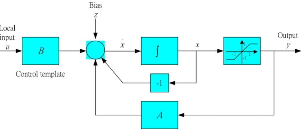
(11) 1. Introduction. 1.1. Motivation The two-dimensional inputs and outputs of the Cellular Neural Networks (CNN) [1], [2], make it very suitable for image processing. A single CNN can solve a basic task such as thresholding and filtering, etc. However, either from application or biologics points of views, several CNNs in parallel or in series can solve more complex intelligent problems, such as edge detection with impulse noise, the detection of fuzzy boundary, and features extraction, etc. To solve more complex problems, several CNNs can be integrated to solve specific problem. In this thesis, we propose a novel framework to integrate a set of CNNs in parallel in order to solve more complex intelligent problems.. 1.2. Cellular Neural Network The CNN first introduced as one that is able to implement alternative to fully connected neural networks, has evolved into a paradigm for these types of arrays. The block diagram of the CNN is shown in Fig. 1.1, and its dynamics is described by the following differential equations: d xi , j (t ) = − xi , j (t ) + ∑ a k ,l y i + k , j +l (t ) + ∑ bk ,l ui + k , j +l (t ) +zi , j dt k ,l∈N r k ,l∈N r N r (i, j ) = {C ( k , l ) | max{| k − i |,| l − j |} ≤ r}. (1.1) (1.2). with output nonlinearity. 1 y i , j (t ) = (| xi , j (t ) + 1 | − | xi , j (t ) − 1 |) , 2 1. (1.3).

(12) Bias. z Local input. u. Output. .. x. B. ∫. x. y. 1 -1. -1. 1. Control template -1. A Feedback template. Figure 1.1 Block diagram of a CNN. where xi , j is the internal state of a cell, y i , j is the output, ui , j is external input and. zi , j is a local value called bias, (i, j) is a grid point associated with a cell on the 2-D grid, and (k, l) is a grid point in the neighborhood within a radius r of the cell (i, j). That is, C(k, l) is a cell in the neighborhood within a radius r of the cell C(i, j) and N r (i, j ) is a set including all C(k, l) associated with a cell C(i, j). The A and B are. two generic parametric functions called feedback template and control template, respectively. A CNN has a space invariant local interconnection structure associated with 19 free parameters (neighborhood within a radius r = 1), which exclusively determines the dynamic behavior of the CNN. The CNN possesses some important characteristics such as efficient real-time processing capability and feasible VLSI implementation. Some applications requiring high-speed processing include real-time object recognition and tracking, high-speed visual inspection of manufacturing processes, etc.. 1.3. CNN Integrated System Besides some basic image processing tasks, the CNN has been used to mimic the 2.

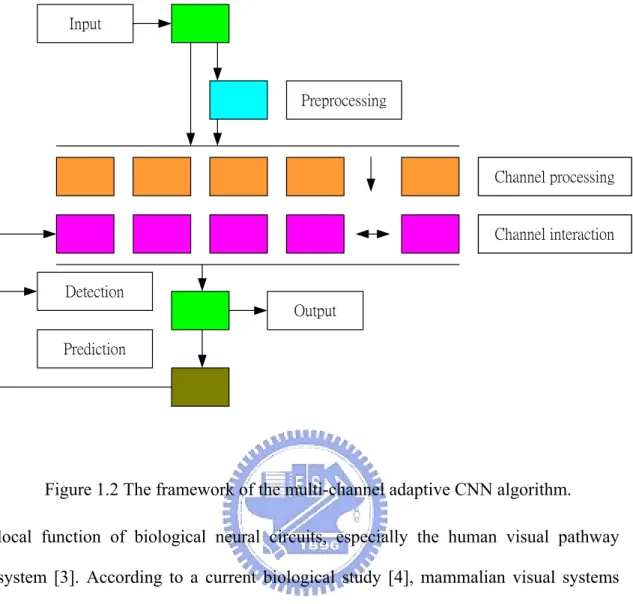
(13) Input. Preprocessing. Channel processing. Channel interaction. Detection Output Prediction. Figure 1.2 The framework of the multi-channel adaptive CNN algorithm. local function of biological neural circuits, especially the human visual pathway system [3]. According to a current biological study [4], mammalian visual systems process the world through a set of separate parallel channels. As shown in Fig. 1.2, each sub-channel can be regarded as a unique CNN. The output of these sub-channels is then combined to form the new channel responses. One key point is to define the global channel interaction and result in a unique binary image flow. As a result, it is widely accepted that using a set of CNNs in parallel can achieve higher-level information processing and reasoning functions either from biologics or application points of views. Such an integrated CNN system can solve more complex intelligent problems. For designing an integrated CNN system, in addition to the determination of a set of templates, another kernel problem is the way of integration. To solve this problem, the fuzzy inference system (FIS) is gaining attention. The FIS is a popular 3.

(14) computing framework based on the concept of fuzzy set theory, fuzzy if-then rules, and fuzzy reasoning. With crisp inputs and outputs, fuzzy inference system implements a nonlinear mapping from its input space to output space by a number of if-then rules. It is very useful in image processing when it is difficult to specify, in a crisp mathematical form, the operation that is needed to yield a satisfying result from a complex image. For example, the boundary detection of different regions strongly depends on a subjective decision, especially in medical image. It cannot be clearly defined what is an edge-like and what is a noise-like pattern. In many cases both statements might be true; therefore a fuzzy-type linguistic description of all patterns is better than a crisp set approach. Therefore, FIS can play an important role to integrate a set of CNNs into a system.. 1.3.1. Existing Fuzzy-based CNN Models and CNN Integrated Systems To make a CNN or a set of CNNs have the ability of reasoning functions, several fuzzy-based CNN models were proposed [5]-[9], which are fuzzy cellular neural network (FCNN) proposed by Yang et al [5], [6], fuzzy reasoning implemented on CNN proposed by Balsi et al [7], [8]. To make a set of CNNs in parallel achieve higher-level information processing, several integrated CNN systems are proposed [9]-[11], which are cellular neuro-fuzzy networks (CNFNs) proposed by Colodro [9], and fuzzy-type CNN proposed by Rekeczky [10], [11] and Szatmári et al. [4]. In the following, we will survey these related papers.. 4.

(15) 1.3.1.1. Existing Fuzzy-based CNN Models Yang et al. [5], [6] first proposed a FCNN model in 1996. Such architecture had the same structure as a CNN with nonlinear connections, but the connection functions were stated in terms of fuzzy logic operators, so that the model departed from the trend towards standardization and simplification of connection functions to be realized in future CNN universal machine (CNN-UM) chips. The authors gave an example for edge detection. The characteristics of Yang’s FCNN are to integrate fuzzy logic into the structure of traditional CNN and maintains local connection among cells, but its drawback is that it is too complex to implement in the short term. Balsi et al. [7], [8] proposed a fuzzy reasoning method implemented on CNN-UM in 1999. Such architecture has the same structure as a conventional CNN. The authors showed that standard fuzzy logic could be straightforwardly implemented in the CNN-UM framework without any architectural modifications. The authors showed several examples for edge detection and noise removal. One of them concerned the edge detection in the presence of impulse noise. Experimental result showed the edge could be detected even impulse noise existed with appropriate fuzzy rules. The characteristic of Balsi’s FCNN is to map a standard Sugeno-style fuzzy-rule-based image processing algorithm into a standard CNN-UM analogic (analog and logic) algorithm. However, the fuzzy rules must be obtained by domain experts. Yang et al. [5], [6] and Balsi et al. [7], [8] were devoted to make a CNN or a set of CNNs have the ability of fuzzy reasoning. However, the other authors [4], [9]-[11] were devoted to make a set of CNNs in parallel achieve higher-level information processing, which is the main research subject in this thesis. The related papers are described in the following subsection. 5.

(16) 1.3.1.2. Existing CNN Integrated Systems In 1996, Colodro et al. [9] proposed a new class of cellular networks called cellular neuro-fuzzy networks (CNFNs), which the linear combination and piece-wise linear function of a CNN were replaced by an arithmetic fuzzy-logic unit. To demonstrate the capabilities of the proposed CNFN, the authors gave an application example for edge detection. The example used eight fuzzy rules and its CNFN templates were well-known Sobel masks to detect edge. The characteristic of Colodro’s CNFN is to provide a new architecture based on CNN and FIS to solve problem. Its drawbacks are the templates cannot be learned and the fuzzy rules must be obtained by domain experts. Though Colodro et al. showed a simple example for edge detection, they presented an approach to integrate different CNN template sets to solve problem. Rekeczky et al. [10], [11] developed a common CNN framework for various adaptive non-linear filters [10]. Their experimental results indicated that impulsive noise elimination will be more robust if both the pixel intensity and the edge-like local property is taken into consideration and exploited in a fuzzy-type decision. Rekeczky et al. [11] also proposed a CNN-based spatio-temporal approach to find the endocardial (inner) boundary of the left ventricle from a sequence of echocardiographic images. The kernel of the left ventricle was located and the boundary was found using a fuzzy-adaptive technique. Boundary dislocation, area and smoothness constraints were transformed into the transient length of the CNN while the a priori knowledge about the heart morphology was built into the spatial template parameters. The authors showed the architecture of the processing steps of a fuzzy-type CNN analogic algorithm. As observed by Rekeczky et al. [11], it was not necessary to use a specialized CNN model [5], [6] in order to exploit fuzzy logic 6.

(17) concepts. The reasons were as follows. First, elementary fuzzy-type computations, such as the min and max operator, are already defined in CNN-based gray-scale morphology and require only simple non-linear templates with sigmoid-type nonlinear interactions. Second, higher level fuzzy strategies can also be synthesized using ‘conventional’ linear and non-linear CNN templates. The characteristic of Rekeczky’s fuzzy-type CNN analogic algorithm is to use FIS to integrate different CNNs to detect fuzzy boundary of a given object. Similarly, its drawbacks are the corresponding templates cannot be learned and must be assigned in advance, and the fuzzy rules must be obtained by domain experts. In 2003, Szatmári et al. [4] proposed an image flow processing mechanism for visual exploration systems. The goal of this multi-channel topographic approach was to produce decision maps for salient feature localization and identification. According to a current biological study, mammalian visual systems process the world through a set of separate parallel channels. Each sub-channel can be regarded as a unique CNN. The output of these sub-channels is then combined to form the new channel responses. In the core of the algorithm crisp or fuzzy logic strategies define the global channel interaction and result in a unique binary image flow. Experimental results were shown for terrain exploration environment based on multiple feature extraction. The characteristic of Szatmári’s method is to use FIS to integrate different CNNs to extract features of a given object. Similarly, its drawbacks are the corresponding templates cannot be learned and the fuzzy rules must be obtained by domain experts.. 1.3.2. The Proposed CNN Integrated System Two common characteristics are observed in the representative works of integrated CNN systems such as Colodro et al. [9] and Roska et al. [4], [11]. First, 7.

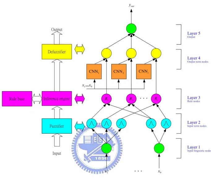
(18) they all used many CNNs in parallel to solve a complex problem such as edge detection with impulse noise, the detection of fuzzy boundary, and features extraction, etc. Second, they all used FIS to make a final decision. For building a FIS, we have to specify the fuzzy sets, fuzzy operators and the knowledge base. However, the existing methods [4], [9], [11] all need to manually take the fuzzy rules by domain experts, which is difficult, even for domain experts, to examine all the input–output data from a complex system to find a number of proper fuzzy rules. In addition, they all need to assign the corresponding templates of CNNs in advance (i.e., templates cannot be learned with fuzzy rules simultaneously). Although according to Nossek’s survey [12], the template coefficients of a CNN can be found by design [12], [13] or by learning [12], [14], these techniques cannot be applied to the design or learning of an integrated CNN system directly. To cope with these drawbacks, we introduce a novel framework for automatically constructing a multiple-CNN integrated neural system in the form of a recurrent fuzzy neural network (FNN) called recurrent fuzzy CNN (RFCNN). Figure 1.3 shows the structure of the RFCNN and its functional correspondence with a typical fuzzy inference system (FIS) [15]-[17], where the fuzzifier is to transform crisp measured data into suitable linguistic values, which are then matched with the fuzzy rules in the rule base by performing fuzzy approximate reasoning to achieve desired linguistic outputs, which are then transformed back to final crisp outputs through the defuzzifier. The RFCNN shown in Fig. 1.3 can automatically learn its proper network structure and parameters simultaneously. The structure learning includes the fuzzy division of the problem domain and the creation of fuzzy rules and CNNs. The parameter learning includes the tuning of fuzzy membership functions and CNN templates. In the RFCNN, each learned fuzzy rule corresponds to a CNN. Hence, each CNN takes care of a fuzzily separated problem region, and the functions of all 8.

(19) yout. Output. Layer 5 Output. Defuzzifier Layer 4. Output term nodes. CNN i. CNN 2. CNN1 x1 ... x9. Rule base. R1. Inference engine. .... R2. Layer 3. Ri. Rule nodes. Layer 2. Fuzzifier. Input term nodes. Layer 1. Input linguistic nodes. Input. x1. .... x9. Figure 1.3 The schematic diagram of the RFCNN and FIS.. CNNs are integrated through the fuzzy inference mechanism. The RFCNN is constructed in the form of a recurrent FNN. Two important learning tasks of a FNN are the structure identification and the parameters identification [15]-[19]. The structure identification is the partition of the input-output space [20]-[23], which influences the number of generated fuzzy rules, each corresponding to a CNN. Efficient partition of input-output data will result in faster convergence and better performance for FNN. In the parameter learning of the 9.

(20) RFCNN, the ordered-derivative calculus is applied to derive the recurrent learning rules due to the recurrent structure of the RFCNN inherited from CNNs. The derived rules can learn the CNN templates and other parameters in the RFCNN efficiently. The proposed RFCNN provides a solution to the current dilemma on the decision of templates and/or fuzzy rules in the existing integrated (fuzzy) CNN systems. It has been applied to solve the real-world defect inspection. This is an application for the defect inspection of color filter, which contains multiple types of defects (faults) with different features on a single image. Experimental results, shown in Sections 4 of Chapter 2 and Chapter 3, successfully demonstrate that the introduced scheme is very effective and promising.. 1.4. Concluding Remarks In this chapter, several fuzzy-based CNN integrated system are presented. Since those methods suffered from two problems, i.e., they all need to assign the corresponding templates of CNNs in advance (i.e., templates cannot be learned) and they all need to take the fuzzy rules manually by domain experts. To cope with these drawbacks, we proposed a novel framework for automatically constructing a multiple-CNN integrated neural system in the form of a recurrent fuzzy neural network (FNN). This system, called recurrent fuzzy CNN (RFCNN) [13], can automatically learn its proper network structure and parameters simultaneously. Each CNN takes care of a fuzzily separated problem region, and the functions of all CNNs are integrated through the fuzzy inference mechanism. For learning algorithm, the details of structure-learning algorithm based on adaptive ICA (independent component analysis) mixture-model technique are described in Section 3.1 of Chapter 2; the details of parameter-learning algorithm are described in Sections 3.2 of Chapter 10.

(21) 2 and Chapter 3, respectively. For experimental results and discussions, they are described in Sections 4 of Chapter 2 and Chapter 3, respectively. Finally, conclusions and perspectives are described in the last chapter.. 11.

(22) 2. A Recurrent Fuzzy Cellular Neural Network System with Automatic Structure and Template Learning. In this chapter, we propose a novel framework for automatically constructing a multiple-CNN integrated neural system in the form of a recurrent fuzzy neural network. This system, called recurrent fuzzy CNN (RFCNN), can automatically learn its proper network structure and parameters simultaneously. The structure learning includes the fuzzy division of the problem domain and the creation of fuzzy rules and CNNs. The parameter learning includes the tuning of fuzzy membership functions and CNN templates. In the RFCNN, each learned fuzzy rule corresponds to a CNN. Hence, each CNN takes care of a fuzzily separated problem region, and the functions of all CNNs are integrated through the fuzzy inference mechanism. The new on-line adaptive ICA (independent component analysis) mixture-model technique, proposed in Section 3.1 of this chapter, is used for the structure learning of RFCNN, and the ordered-derivative calculus is applied to derive the recurrent learning rules of CNN templates in the parameter-learning phase. The proposed RFCNN provides a solution to the current dilemma on the decision of templates and/or fuzzy rules in the existing integrated (fuzzy) CNN systems. The capability of the proposed RFCNN is demonstrated on the real-world defect inspection problems. Experimental results show that the proposed scheme is effective and promising.. 12.

(23) 2.1. Introduction The CNN has been used to mimic the local function of biological neural circuits, especially the human visual pathway system [3]. According to a current biological study [4], mammalian visual systems process the world through a set of separate parallel channels. Each sub-channel can be regarded as a unique CNN. The output of these sub-channels is then combined to form the new channel responses. As a result, it is widely accepted that using a set of CNNs in parallel can achieve higher-level information processing and reasoning functions either from biologics or application points of views. Such an integrated CNN system can solve more complex intelligent problems. For designing an integrated CNN system, in addition to the determination of a set of templates, another kernel problem is the way of integration. To solve this problem, the fuzzy inference system (FIS) can play an important role to integrate a set of CNNs into a system. As mentioned in Section 3 of Chapter 1, to make a set of CNNs in parallel achieve higher-level information processing, several integrated CNN systems are proposed [4]-[7]. They have two common characteristics. First, they all used many CNNs in parallel to solve a complex problem. Second, they all used FIS to make a decision. The common drawbacks of these approaches are that they all need to assign the corresponding templates of CNNs in advance (i.e., templates cannot be learned) and they all need to take the fuzzy rules manually by domain experts. Although according to Nossek’s survey [8], the template coefficients of a CNN can be found by design [8], [9] or by learning [8], [10], these techniques cannot be applied to the design or learning of an integrated CNN system directly. To cope with these drawbacks, we proposed a novel framework for automatically constructing a multiple-CNN integrated neural system in the form of a recurrent fuzzy 13.

(24) neural network (FNN) [11], [12]. This system, called recurrent fuzzy CNN (RFCNN) [13], can automatically learn its proper network structure and parameters simultaneously. The structure learning includes the fuzzy division of the problem domain and the creation of fuzzy rules and CNNs. The parameter learning includes the tuning of fuzzy membership functions and CNN templates. In the RFCNN, each learned fuzzy rule corresponds to a CNN. Hence, each CNN takes care of a fuzzily separated problem region, and the functions of all CNNs are integrated through the fuzzy inference mechanism. As mentioned in Section 3 of Chapter 1, the RFCNN is constructed in the form of a recurrent FNN, which includes two important learning tasks: the structure identification and the parameters identification [15]-[19]. In this chapter, the new on-line adaptive ICA (independent component analysis) mixture-model technique, described in Section 3.1, is used for the structure learning of the RFCNN. Basically, ICA finds directions in the input space which lead to independent components instead of just uncorrelated ones, as PCA (principle component analysis) does [24], [25], so it reduces not only the number of rules (i.e., CNN) but also the number of membership functions under a pre-specified accuracy requirement dynamically. In the parameter learning of the RFCNN, the ordered-derivative calculus is applied to derive the recurrent learning rules due to the recurrent structure of the RFCNN inherited from CNNs [1], [2]. The derived rules can learn the CNN templates and other parameters in the RFCNN efficiently. The proposed RFCNN provides a solution to the current dilemma on the decision of templates and/or fuzzy rules in the existing integrated (fuzzy) CNN systems. It has been applied to solve the real-world defect inspection problems, which contain multiple types of defects (faults) with different features on a single image. Experimental results successfully demonstrate that the proposed scheme is very effective and promising. 14.

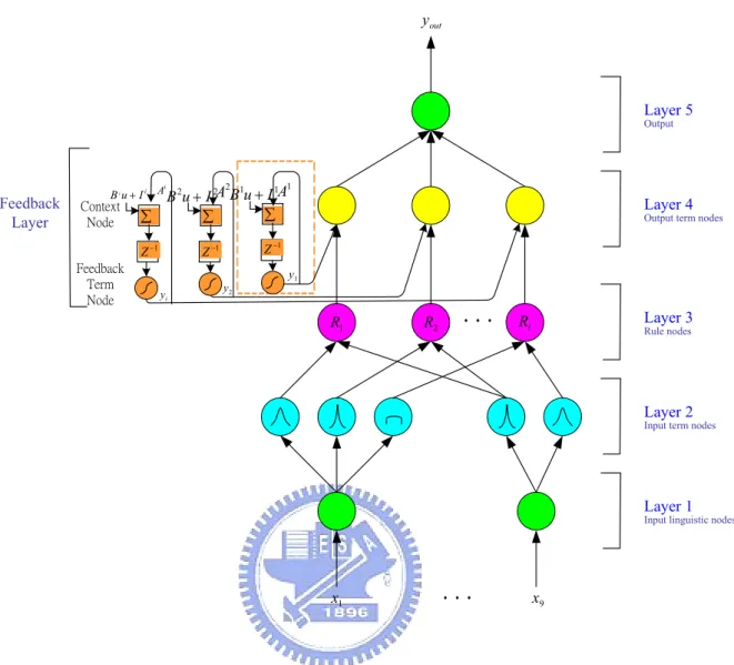
(25) This chapter is organized as follows. Section 2 describes the structure and functions of the proposed RFCNN. Section 3 describes the on-line structure and parameters learning algorithm for the RFCNN. Section 4 gives experimental results and discussions. Finally, conclusions are summarized in the last section.. 2.2. Structure of the RFCNN In this section, the structure of the proposed RFCNN shown in Fig. 2.1 is introduced. For clarity, we consider a CNN, with time constant = 1, time step = 1, and neighborhood within a radius = 1, which is characterized by the following templates: 0 0 i i  A = 0 a 0, 0  0 0. b i −1, −1 b i −1,0 0  0  , B i =  b i 0 , −1 b i 0 , 0   b i 1, −1 b i 1,0 0 . b i −1,1   b i 0,1 , I i = z i , b i 1,1 . (2.1). where Ai , B i , and z i is feedback template, control template, and bias of the ith CNN, respectively. By defining a CNN as above, the six-layered RFCNN network will realize a fuzzy model of the following form: Rule i :. IF x1 is M 1i and … x j is M ij … and x9 is M 9i THEN yi (t + 1) is f ' ( Ai y i (t ) + B i u(t ) + z i (t )). (2.2). or Rule i : IF x1 is M 1i and … x j is M ij … and x9 is M 9i THEN. yi (t + 1). is. f ' ( a0i ,0 yi (t ) + b i −1, −1 x1 (t ) + b i −1, −0 x 2 (t ) + ... + b i 1,1 x9 (t ) + z i (t )) ,. (2.3) where the current input vector is u = x t = [ x1, ..., x9 ]T , Ai yi (t ) is a 0i ,0 y i (t ) ,. B i u(t ) is. ∑ b u =b i. i. x (t ) + bi −1, −0 x2 (t ) + ... + b i1,1 x9 (t ) , f ' is a sigmoid function,. −1, −1 1. M ij is a fuzzy set, and a 0i ,0 , b i k ,l , and z i are consequent parameters representing 15.

(26) yout. Layer 5 Output. Feedback Layer. Feedback Term Node. 2. 1 1. ∑. I 2A B u + I A ∑ ∑. Z −1. Z −1. i B i u + I i A B 2u +. Context Node. yi. 1. Layer 4. Output term nodes. Z −1 y2. y1. R1. R2. .... Layer 3. Ri. Rule nodes. Layer 2. Input term nodes. Layer 1. Input linguistic nodes. x1. .... x9. Figure 2.1 Structure of the proposed RFCNN. feedback template, control template, and bias of the ith CNN, respectively. The number of input dimension of the RFCNN will be (2r + 1) if the neighborhood of a 2. CNN cell is within a radius = r. As shown in (2.3), we focus on uncoupled CNN cells in this chapter. With this six-layered network structure of the RFCNN, we shall define the function of each node and use the proposed on-line ICA mixture model described in the next section to construct the structure of the RFCNN. The RFCNN consists of nodes, each of which has some finite “fan-in” of connections represented by weight values from other nodes and “fan-out” of connections to other nodes. Associated with the fan-in of a node is an integration 16.

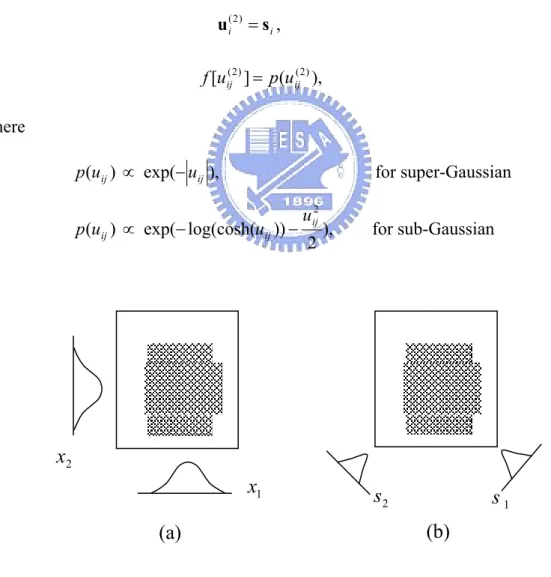
(27) function f , which serves to combine information, activation, or evidence from other nodes. This function provides the net input for this node. node − input = f [ u1( k ) , u 2( k ) , ..., u (pk ) ; w1( k ) , w 2( k ) , ..., w (pk ) ] ,. (2.4). where u1( k ) , u 2( k ) , ..., u (pk ) are inputs to this node and w1( k ) , w2( k ) , ..., w (pk ) are the associated link weights. The superscript (k ) in (2.4) indicates the layer number. This. notation will also be used in the following equations. A second action of each node is to output an activation value as a function of its net-input node − output ( k ) = oi( k ) = a ( k ) (node − input ) = a ( k ) ( f ) ,. (2.5). where a (⋅) denotes the activation function. We shall next describe the functions of the nodes in each of the six layers of the RFCNN, which include five feedforward layers and one feedback layer. Layer 1: No computation is done in this layer. Each node in this layer, which corresponds to one input variable, only transmits input values to the next layer directly. That is f = ui(1) , and oi(1) = a (1) ( f ) = f .. (2.6). From the above equation, the link weight in layer one [ wi(1) ] is unity. Layer 2: Each node in this layer corresponds to one linguistic value (small, large, etc.) of one of the input variables in Layer 1. In other words, the membership value which specifies the degree to which an input value belongs a fuzzy set is calculated in Layer 2. There are many choices for the types of membership functions for use, such as triangular, trapezoidal, or Gaussian ones. In this chapter, the membership functions are determined by the on-line ICA mixture model, which are either super-Gaussian 17.

(28) function or sub-Gaussian function. It is noted that the output x from Layer 1 is projected into the independent axes obtained by the on-line ICA mixture model (as shown in Fig. 2.2) such that. si = Bi x ,. (2.7). where B i is the basis matrix determined by the on-line ICA mixture model, i = 1, 2, ..., J , and J is the number of clusters. That is, if the input data are classified into J clusters, the number of rules will be J . With the choice of non-Gaussian membership function, the operation performed in this layer is. u i( 2 ) = s i , f [u ij( 2 ) ] = p (u ij( 2 ) ),. where p(uij ) ∝ exp(− uij ),. for super-Gaussian. p (u ij ) ∝ exp(− log(cosh(u ij )) −. uij2 2. ),. for sub-Gaussian. x2 x1. s2. s1 (b). (a). Figure 2.2 Transformation by the on-line ICA mixture model for the proposed RFCNN. (a) The regions covered by the original axes. (b) The covered regions by the independent axes obtained by the on-line ICA mixture model transformation. 18.

(29) and oi( 2) = a ( 2 ) ( f ) = f ,. (2.8). where u ij is the transformed value of the jth term of the ith input variable x i . The transformation can be regarded as a change of input coordinates, where the parameters of each membership function are kept unchanged, i.e., the center and the width of each membership function on the new coordinate axes are the same as the old ones. Layer 3: A node in this layer represents one fuzzy logic rule and performs precondition matching of a rule. Here, we use the following AND operation for each Layer-3 node f [ui( 3) ] = ∏ ui( 3) , i. and oi( 3) = a ( 3) ( f ) = f .. (2.9). The link weight in the Layer 3 [ wi( 3) ] is unity. The output f of a Layer-3 node represents the firing strength of the corresponding fuzzy rule. Layer 4: This layer is called the consequent layer. Different nodes in Layer 3 may be connected to the same node in Layer 4, meaning that the same consequent fuzzy set is specified for different rules. One of the inputs to each node is the output delivered from Layer 3 (firing strength) and the other inputs are CNN related inputs a ( 6 ) , which are the output of feedback term node. The feedback term node will be described in the feedback layer part in this section. Combining the two kinds of inputs in Layer 4, we obtain the whole function performed by this layer as f [ui( 4 ) ] = ui( 4 ) , and 19.

(30) oi( 4 ) = a ( 4 ) ( f ) = a ( 6 ) ⋅ f = sigmoid ( Ai yi (t ) + B i u(t ) + z i (t )) ⋅ f ,. (2.10). where Ai , B i , z i is feedback template, control template, bias of the ith CNN, respectively, as defined in (2.1), and sigmoid () is a sigmoid function, as defined in (2.13). Layer 5: Each node in this layer corresponds to one output variable. The node integrates all the actions recommended by Layer 4 and acts as a defuzzifier with f [ui( 5) ] = ∑ ui( 5) , i. and y out = o ( 5) = a ( 5) ( f ) = f. . (2.11). Feedback Layer: As shown as Fig. 2.1, this self-feedback layer characterizes the consequents of the RFCNN as a CNN template. Two types of nodes are used in this layer, the square node named as context node and the circle node named as feedback term node, where each context node is associated with a feedback term node. The number of context nodes (and thus the number of feedback term nodes) is the same as that of output term nodes in layer 4. The inputs to a context node are from its corresponding output term nodes ( y i (t ) ), the input variables from Layer 1 ( u(t ) = x t (t ) = [ x1, ..., x9 ]T ), and template bias ( z i (t ) ). The output of its associated feedback term node is fed to the original node in layer 4. The context node functions as the state (the summation of input part) of the ith CNN x i (t + 1) = Ai yi (t ) + B i u(t ) + z i (t ) .. (2.12). As to the feedback term node, the membership function f (u ) = 2 /(1 + e −2 u ) − 1 is used to approximate piece-wise linear function used in CNN. With this choice, the feedback term node evaluates the output by 20.

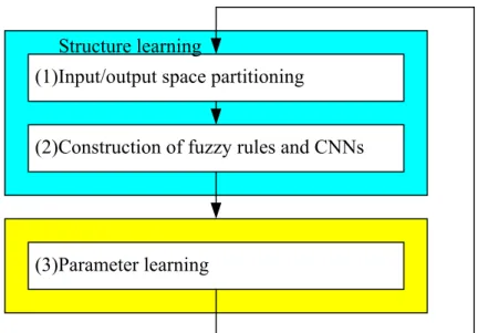
(31) oi( 6 ) = a ( 6 ) =. 2 1 + e −2 x. i. −1 .. (2.13). This output is connected to its corresponding node in layer 4, which characterizes the consequents of the RFCNN as a CNN template.. 2.3. Learning Algorithm for the RFCNN Two types of learning, structure and parameter learning, are used concurrently for the RFCNN. The structure learning includes both the precondition and consequent structure identification of a fuzzy if-then rule. In the RFCNN, the structure learning includes the fuzzy division of the problem domain (precondition structure identification), and the creation of fuzzy rules and CNNs (consequent structure identification). The precondition structure identification corresponds to the input-space partitioning and can be formulated as a combinational optimization problem with the following two objectives: to reduce the number of rules generated and to reduce the number of fuzzy sets on the universe of discourse of each input variable. As to the consequent structure identification, the main task is to decide when to generate a new consequent term (or a new CNN) for the output variable. In our system, we propose an on-line ICA mixture model to realize the precondition and consequent structure identification part of the RFCNN. For the parameter learning, the parameters of each CNN template in the consequent parts are adjusted by the ordered derivative algorithm to minimize a given cost function. The parameters in the precondition part are adjusted by the on-line ICA mixture model algorithm. The RFCNN can be used for normal operation at any time during the learning process without repeated training on the input-output patterns when on-line operation is required. There are no rules (i.e., no nodes in the network except the input-output nodes) in this network initially. They are created dynamically 21.

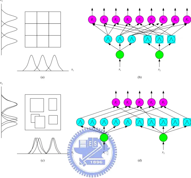
(32) Structure learning (1)Input/output space partitioning (2)Construction of fuzzy rules and CNNs. (3)Parameter learning. Figure 2.3 Flowchart of the learning algorithm for the proposed FNN. as learning proceeds upon receiving on-line incoming training data by performing the following learning processes simultaneously (see Fig. 2.3). As shown in Fig. 2.3, learning processes (1) and (2) belong to the structure learning phase and (3) belongs to the parameter learning phase. The details of these learning processes are described in the rest of this section.. 2.3.1. Structure Learning Algorithm of RFCNN. 2.3.1.1 Input/Output Space Partitioning Efficient partition of input-output data will result in faster convergence and better performance for the RFCNN. The most direct way is to partition the input space into grid types and each grid represents a fuzzy if-then rule (see Fig. 2.4(a)). This is called grid-based partitioning. The major problem of such kind of partition is that the number of fuzzy rules (and thus the number of CNNs) increases exponentially if the number of input variables or that of partition increases. A flexible partition method, 22.

(33) the clustering-based approach which clusters the input training vectors in the input space, will reduce the rule and CNN numbers [20]-[23]. In fact, by observing the projected membership functions in Fig. 2.4(c), although the number of membership functions in Fig. 2.4(d) is more than that in Fig. 2.4(b), there are only 5 rules in Fig. 2.4(d); however, there are 9 rules in Fig. 2.4(b). By observing the projected membership functions in Fig. 2.4(c), we find that some membership functions projected from different clusters have high similarity degrees. These highly similar membership functions can be checked and merged by similarity measure [23]. In the rest of this subsection, we will introduce some clustering methods such as C-means, ISODATA, and a new on-line ICA mixture model to provide a proper partition of the input-output space for the RFCNN [25]. These clustering algorithms will be briefly described in the following subsections.. 23.

(34) x2. R1. R2. R3. R4. R5. R6. x1. x1. R7. R8. R9. x2. (a). (b). x2. R1. x1. R2. R3. x1. (c). R4. R5. x2 (d). Figure 2.4 Fuzzy partitions of two-dimensional input space. (a) Grid-based partitioning. (b) If-then rules based on grid-based partitioning (c) Clustering-based partitioning. (d) If-then rules based on clustering-based partitioning.. 2.3.1.1.1 C-means Clustering In the C-means clustering algorithm, the sum of the squared distances from all of the points in the cluster to the cluster center is used as the criterion for grouping input data samples. The algorithm can be described as follows: Step 1. Choose C initial cluster centers. For the first iteration, the starting values for cluster centers are chosen randomly.. 24.

(35) Step 2. Assign unknown samples to corresponding clusters. For each sample, the Euclidean distance from each cluster center is calculated, and the sample is assigned to the cluster with the minimum distance. Step 3. Compute new cluster centers, which are calculated by the mean value of the points in the same cluster. Step 4. Check for the condition of convergence, which is that no cluster center has changed its value during Step 3. The C-means algorithm is a simple and efficient scheme to find proper input/output partitioning for the RFCNN, and then determine the proper fuzzy rules (i.e., CNNs). However, it assumes that the number of clusters is known in advance, which is exactly what we have to know from the clustering algorithm to obtain the number of fuzzy rules (i.e., CNNs) in the RFCNN in some real-world applications. As a result, the C-means algorithm cannot be used to on-line determine the structure of the RFCNN if there is such a need.. 2.3.1.1.2 ISODATA In the ISODATA (Iterative Self-Organizing Data Analysis Technique) clustering algorithm [26], like the C-means algorithm, cluster centers are updated iteratively. The ISODATA algorithm is a good method to determine the structure of the RFCNN though it is more complex, because some heuristic procedures are incorporated into it. Three additional procedures that the algorithm performs are as follows: (1) if a cluster contains a small number of samples, that cluster is discarded; (2) if a cluster contains a large number of samples and the standard deviation is large, then the cluster is split into two; and (3) if the distance between two cluster centers is small, then the clusters are merged into one. Essentially, what is done in the ISODATA algorithm is that very small clusters are discarded, very large clusters are split, and very close clusters are 25.

(36) merged. Again, like the C-means algorithm, the proper cluster number should be known in advance before applying the ISODATA algorithm. This also hinders the use of this clustering algorithm on the on-line structuring learning of RFCNN in some real-world problems.. 2.3.1.1.3 On-line ICA Mixture Model for Dynamic Clustering 1) ICA Mixture Model Several methods for input space partition have been proposed to cluster the input training vectors in the input space, such as Kohonen learning rule, hyperbox method, product-space partitioning, fuzzy c-mean method, EM algorithm, etc. [26]-[29]. Those methods are usually based on Gaussian membership functions. In general, the observed data can be categorized into several mutually exclusive classes [30]. When the data in each class are modeled as multivariate Gaussian, it is called a Gaussian mixture model (GMM) which is widely used throughout the fields of machine learning and statistics. One major drawback of GMMs is that if the dimension d of the problem space increases, the size of each covariance matrix, d2, becomes prohibitively large. This problem has been solved by Tipping and Bishop [31] who replaced each Gaussian with a probabilistic principal component analysis (PCA) model. This allowed the dimensionality of each covariance to be effectively reduced while maintaining the richness of the model class. Independent component analysis (ICA) [24] is a technique that exploits higher-order statistical structure of the data, which has recently gained attention due to its successful applications to signal processing problems including speech enhancement, discrete signal processing and image processing, etc. The goal of ICA is to linearly transform the data such that the transformed variables are as statistically independent from each other as possible. 26.

(37) Basically, it finds direction in the input space which lead to independent components instead of just uncorrelated ones as PCA does, so it can be used to reduce not only the number of rules but also the number of membership functions under a pre-specified accuracy requirement dynamically. Another drawback of GMMs is that it is based on Gaussian function. In some situation, it could not be separated from each other. It is generalized by assuming the data in each class are generated by a linear combination of independent non-Gaussian source [33]. This model is called the ICA mixture model. This allows modeling of classes with non-Gaussian structure such as platykurtic or leptokurtic probability density functions, and the model uses the gradient ascent method to maximize the log-likelihood function. In previous applications, this approach showed improved performance in data classification problems [34] and learning efficient codes for representing different types of images [25]. The advantage of this model is that the input data with increasing numbers of classes can provide greater flexibility in modeling structure and in finding more features compared with Gaussian mixture models or standard ICA algorithms. Although the ICA mixture model has many advantages, its cluster number should be given beforehand and the learning scheme is only suitable for off-line instead of on-line operation. Therefore, in the following section, we shall propose an on-line ICA mixture model to provide better dynamic partitioning of the input-output space for the proposed RFCNN.. 2) On-line ICA Mixture Model for Dynamic Clustering The proposed on-line ICA mixture model is derived from the conventional ICA mixture model. To enable the on-line operation, we will define a criterion to determine whether the number of clusters should be increased or not for any incoming training pattern. For each incoming pattern to the RFCNN, the resulting firing 27.

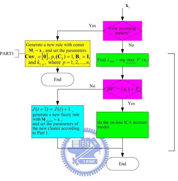
(38) strength of a fuzzy rule can be interpreted as the degree that the incoming pattern belongs to the corresponding cluster. This likelihood can be represented as. F j ( x t ) = ln p( x t C j ) ,. (2.14). where x t denotes the incoming pattern at time t , and ln p( x t C j ) is the log likelihood value indicating the degree that the input data, x t , belongs to the jth cluster for j ∈ [1, J ] . Now, we assume that the number of clusters at time t is J (t ) . Then, the total probability at time t is J (t ). (. ). (. ). p (x t ) = ∑ p x t C j pt (C j ) .. (2.15). j =1. Therefore, the posterior probability is:. (. ). p C j xt =. p xt C j pt −1 (C j ) p(xt ). ,. (2.16). where p t −1 (C j ) is the prior probability at preceding time, which can be obtained by former calculation result of the jth cluster. Hence, the probability pt (C j ) at this moment can be calculated by the following formula: pt (C j ) =. 1 t 1  t −1  p (C j x i ) = ∑ p (C j x i ) + p(C j x t ) ∑ t i =1 t  i =1 . 1 = [(t − 1) ⋅ pt −1 (C j ) + p(C j x t )] t Then the posterior probability p C j x t in (2.16) can be obtained.. (. .. (2.17). ). Based on the above derivation, we can obtain the following criterion for the generation of a new fuzzy rule (i.e., a new CNN). Let x t be the newly incoming pattern at time t . Defining F J max ( x t ) = max F j ( x t ), 1≤ j ≤ J ( t ). (2.18). If F J max ( x t ) < F , then a new rule is generated, where F is a pre-specified 28.

(39) threshold value that decays during the learning process. Once a new rule is generated, the next step is to assign initial values of the corresponding membership functions. If F J max ( x t ) ≥ F , a new incoming data is added to an existed cluster and we have to update the parameters of each cluster such as mean ( M j ), covariance matrix ( Cov j ), and the criterion of data distribution ( k j , p ) that determines if the distribution of data is super-Gaussian or sub-Gaussian with the previous calculation results. They are defined as follows: t −1. ∑ p (C j x i ) x i. ∑ p(C x ) x. t. M j (t ) ≅. =. i =1. ∑ p(C x ) t. j. i =1. i =1. i. j. i. ∑ p(C x ) t. ∑ p(C x )x x j. i =1. j. i. i. − M j (t )M j (t ). T. ∑ p(C x ) j. i. t −1. ∑ p(C x )x x i =1. j. i. T i. t. i =1. i. i. T i. + p (C j x i )x t x Tt. ∑ p(C x ) t. i =1. =. (2.19). − M j (t ))(x i − M j (t )). t. =. + p (C j x t ) x t. T. i. i =1. ≅. i. ∑ p(C x ) i =1. t. Cov j (t ) =. i. t. i. ∑ p(C x )(x j. j. i =1. j. − M j (t )M j (t ). T. (2.20). i. 1 [(t − 1) pt−1 (C j )Cov j (t − 1) + (t − 1) pt−1 (C j ) tpt (C j ). ]. M j (t − 1)M j (t − 1) + p (C j x t )x t x Tt − M j (t )M j (t ) T. 29. T.

(40)  t 2  t 2 ( ) ( ) sech ( ) x p C y i j, p j i  ∑  ∑ p (C j x i )( y j , p (i ) )   i =1   i =1  k j , p (t ) = sign   t  p (C j x i ) ∑  i =1 (2.21) t  p (C j x i )y j , p (i ) ⋅ tanh 2 ( y j , p (i ) ) ∑  − i =1  t  p (C j x i ) ∑  i =1. In the above, the function k j , p (t ) is defined as the function of criterion which allows for automatic switching between super-Gaussian and sub-Gaussian models and (2.21) can be further derived as   T (t )T (t ) 2 − k j , p (t ) = sign  t 1  ∑ p (C j x i )  i =1.  T3 (t )   t p (C j x i ) ∑  i =1. (2.22). where T1 (t ) = ∑ p (C j x i ) sech 2 ( y j , p (i ) ) t. i =1. = T1 (t − 1) + p (C j x t ) sech 2 ( y j , p (t )), T2 (t ) = ∑ p (C j x i )( y j , p (i ) ) t. 2. (2.23). i =1. = T2 (t − 1) + p (C j x t )y j , p (t ), T3 (t ) = ∑ p (C j x i )y j , p (i ) ⋅ tanh 2 ( y j , p (i ) ) t. i =1. = T3 (t − 1) + p (C j x t )y j , p (t )tanh 2 ( y j , p (t )).. Finally, the independent axes B j (t ) , representing the axis of the jth cluster, can be obtained by the following formulations: ∂ ∂ ln p( x t ) = p(C j x t ) ⋅ ln p( x t B j (t − 1), M j (t − 1)) ∂B j ∂B j. [. ]. = p(C j x t ) ⋅ { I − k j , p (t ) ⋅ g ( y j (t )) ⋅ y Tj (t ) ⋅ B j (t − 1)}.. and 30. (2.24).

(41) B j (t ) = B j (t − 1) +. ∂ ln p ( x t ) . ∂B j. (2.25). In (2.24), the function g ( x) is called component-wise nonlinearity function. If the distribution of data is appearing the super-Gaussian distribution, then it will be defined as g ( x) = −2 tanh( x) . Otherwise, if the distribution of data is appearing the sub-Gaussian distribution, then it will be defined as g ( x) = tanh( x) − x . Since the algorithm of on-line ICA mixture model can automatically determine the number of clusters according to new incoming data, it solves the problem of conventional ICA mixture model that the number of clusters has to be given beforehand.. 2.3.1.2. Structure Learning Algorithm of RFCNN with On-line ICA Mixture Model The way the input space is partitioned determines the number of rules extracted from training data as well as the number of fuzzy sets on the universal of discourse of each input variable. We will define a criterion to determine whether a new cluster (i.e., a new fuzzy rule or a new CNN) should be added or not. Let x t of cluster j be the newly incoming pattern at time t . Defining F J max (xt ) = max F j (xt ), 1≤ j ≤ J ( t ). (2.26). where F j (x t ) = ln p( x t C j ) is the log likelihood value indicating the degree that input data, x t , belongs to the jth cluster, and the superscript J max is a maximum log likelihood value among all log likelihood values. If F J max ( x t ) ≥ F , the number of cluster is not increased, where F is a pre-specified threshold value that decays during the learning process. In this case, the new incoming pattern is added to an existed cluster and the parameters of this cluster will be updated properly. Oppositely, 31.

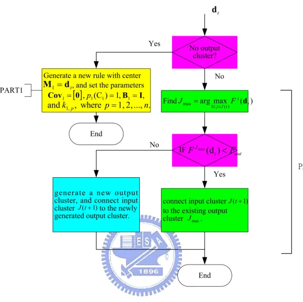
(42) if F J max ( x t ) < F , the number of cluster will be increased. The threshold value F is determined by experiments. The whole algorithm for the generation of new fuzzy rules as well as fuzzy sets in each input variable is shown in Fig. 2.5 step by step. In PART 2 of Fig. 2.5, the threshold Fin determines how many rules will be generated, where Fin should be negative since it is taken in natural log. For a lower value of Fin , more rules will be generated. Similarly, Fout determines how many output clusters will be generated and a lower value of Fout will result in more output clusters. For the output space partitioning, the same approach in (2.14) is used. The generation of a new output cluster corresponds to the generation of a new CNN. Suppose a new input cluster is formed after the presentation of the current input-output training pair (x, d) ; then the consequent part is constructed by the algorithms shown in Fig. 2.6. The above algorithm is based on the fact that different precondition of different rules may be mapped to the same consequent term, i.e., CNN. Since only the center of each output membership function is used for defuzzification, the consequent part of each rule may simply be regarded as a singleton. Compared to the general fuzzy rule-based models with singleton output where each rule has its own individual singleton value, fewer parameters are needed in the consequent part of the RFCNN, especially for the case with a large number of rules.. 32.

(43) xt. Yes. PART1. First incoming pattern?. Generate a new rule with center M1 = x t , and set the parameters. No. Cov1 = [0] , p1 (C1 ) = 1, B1 = I, and k1, p , where p = 1, 2, ..., n.. Find J max = arg max F j ( x t ) 1≤ j ≤ J ( t ). End No. IFF J max ( x t ) < Fin Yes. J (t + 1) = J (t ) + 1 ,. generate a new fuzzy rule with M J ( t +1) = x t , and set the parameters of the new cluster according to Part 1.. do the on-line ICA mixture model.. End. Figure 2.5 Algorithm of input space partitioning.. 33. PART2.

(44) dt. Yes. No output cluster?. Generate a new rule with center. PART1. No. M1 = d t , and set the parameters. Cov1 = [0] , p1 (C1 ) = 1, B1 = I,. and k1, p , where p = 1, 2, ..., n.. Find J max = arg max F j ( d t ) 1≤ j ≤ J ( t ). End No. IF F J max (d t ) < Fout Yes. generate a new output cluster, and connect input cluster J (t + 1) to the newly generated output cluster.. connect input cluster J (t + 1) to the existing output cluster J max .. End. Figure 2.6 Algorithm of output space partitioning.. 2.3.2. Parameter Learning Algorithm of RFCNN by Ordered Derivative Calculus After the network structure is adjusted according to the current training pattern, the network then enters the parameter identification phase to adjust the parameters of the network optimally based on the same training pattern. Notice that the following parameter learning is performed on the whole network after structure learning; no matter whether the nodes (links) are newly added or are existent originally. Since the 34. PART2.

(45) RFCNN is a dynamic system with feedback connections, the backpropagation learning algorithm cannot be applied to it directly. Also, due to the on-line learning property of the RFCNN, the off-line learning algorithms for the recurrent neural networks, like backpropagation through time and time-dependent recurrent backpropagation [17], cannot be applied here. Instead, the ordered derivative [34], which is a partial derivative whose constant and varying terms are defined using an ordered set of equations, is used to derive our learning algorithm. The ordered set of equations, described in Section 2 in each layer, is summarized in (2.28)-(2.33). Our goal is to minimize the error function 1 1 d E (t + 1) = [ yout (t + 1) − yout (t + 1)]2 = ε (t + 1) 2 , 2 2. (2.27). d where y out (t + 1) is the desired output, y out (t + 1) is the current output, and ε (t + 1). d is ( y out (t + 1) − y out (t + 1)) . For each training data set, starting at the input nodes, a. forward pass is used to compute the activity levels of all the nodes in the network to obtain the current output y out (t + 1) . In the followings, dependency on time will be omitted unless emphasis on temporal relationships is required. Summarizing the node functions defined in Section 2, the function performed by the network is y out (t + 1) = ∑ ui( 5). (2.28). i. ( 5). = o ( 4 ) = o ( 6) ⋅ h i ,. (2.29). h i = f [ui( 3) ] = ∏ ui( 3). (2.30). ui. where i. o ( 6) =. 2 1 + e −2 x. i. −1. (2.31). x i (t + 1) = Ai y i (t ) + B i u(t ) + z i (t ) , 35. (2.32).

(46) and (2.1) is redefined as the following equation for clarity: Ai = [0,0,0;0, a i ,0;0,0,0], B ji = [b1i , b2i , b3i ; b4i , b5i , b6i ; b7i , b8i , b9i ] .. (2.33). With the above formula and the error function defined in (2.27), we can derive the update rules for the free parameters in the RFCNN as follows. Update rule of a i (the parameter of feedback template of the ith CNN) is a i (t + 1) = a i (t ) − η. ∂ + E (t + 1) ∂a i. (2.34). + ∂ + E (t + 1) ∂E (t + 1) ∂E (t + 1) ∂ y out ,k (t + 1) = +∑ ∂a i ∂a i ∂a i k ∂y out ,k ( t + 1). (2.35). ∂E (t + 1) ∂ + y out (t + 1) = ∂y out (t + 1) ∂a i. where ∂E (t + 1) = ε (t + 1) , ∂yout (t + 1). (2.36). and (4). ∂ + y out (t + 1) ∂y out (t + 1) ∂ + ok = ∑k ∂o ( 4) ∂a i ∂a i k. (4). =. ∂y out (t + 1) ∂ + oi (4) ∂a i ∂oi. .. (2.37). where. ∂y out (t + 1) ∂ = (4) (4) ∂o i ∂oi. ∑o. (4) k. (t + 1) = 1 ,. (2.38). k. and (4). ∂ + oi ∂a i. =. ∂ [oi( 6 ) ( Aji y i (t ) + B ji u(t ) + z i (t ))]h i i ∂a. .. (2.39). ∂y i (t ) ]} . ∂a i. (2.40). ∂y i (t ) = h (1 + o )(1 − o )[ y i (t ) + a ] ∂a i i. (6) i. ( 6) i. i. Hence, the parameter a i is updated by. a i (t + 1) = a i (t ) − ηε (t + 1){h i (1 + oi( 6 ) )(1 − oi( 6 ) )[ y i (t ) + a i. 36.

(47) Similarly, the parameter b ij (the parameters of control template of the ith CNN) is updated by b ij (t + 1) = b ij (t ) − ηε (t + 1)[h i (1 + oi( 6 ) )(1 − oi( 6 ) ) x j (t )]. (2.41). and the parameter zi (the bias of the ith CNN) is updated by z i (t + 1) = z i (t ) − ηε (t + 1)[h i (1 + oi( 6 ) )(1 − oi( 6 ) )] .. (2.42). As shown in (2.37) to (2.39), the update rules are in recursive form. The value ∂ + y / ∂a is equal to zero initially. For the rest free parameters in the RFCNN, they are obtained during the structure-learning phase by the on-line ICA mixture model algorithm proposed in the last section. Notice that according to the real time recurrent learning (RTRL) scheme [35], we can also obtain the same parameter learning rules for the RFCNN. Of course, other existing on-line learning algorithms [36], [37] for tuning the weights of recurrent neural networks can be possibly adopted for tuning the RFCNN, too.. 2.4. Experimental Results and Discussions The capability of the proposed RFCNN is demonstrated on the real-world defect inspection problems. Automatic defect inspection systems are becoming more and more important in industrial production lines. Especially in electronics industry, an attempt is often made to achieve almost 100% quality control of all components and final goods. Here we are interested in the defect inspection of color filter, which is one of components in TFT-LCD module and gives each pixel of LCD its own color. The difficulties in the defect inspection of color filter are its complex texture and need for high-speed processing. For the reason of high-speed processing, the CNN is a good way to achieve defect inspection. Besides, different kinds of defects in color filter 37.

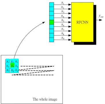
(48) need different CNN templates and some complex defects cannot be detected by a single CNN. Therefore, the proposed RFCNN is a good alternative to detect defect of color filter images. To train the RFCNN, as shown in Fig. 2.7, we use a 3x3 window to get the system inputs and set the whole image as the inputs of the RFCNN. The 3x3 window covers the central pixel and its 8 connected neighbors. The training image and corresponding desired output are shown in Figs. 2.8(a) and 2.8(b). We set the threshold Fin = Fout = −50 and learning rate as η = 0.001 for the clustering algorithm. As mentioned in Section 3, there are no rules (and no CNNs) in the RFCNN initially. They are created dynamically as learning proceeds upon receiving on-line incoming training data by performing the learning processes shown in Fig. 2.3. When the learning processes are done, three clusters (three fuzzy rules and CNN templates) were obtained. For the example of color filter, it takes about 1 minute to learn the structure (interconnection set) and 2 minutes to learn the parameters with Pentium IV 2.0G PC. However, the training can be done off-line, so it is not a problem for the on-line processing of CNN, which causes just little time. x1 x2 x3 x4 x5 x6 x7 x8 x9. yout RFCNN. x1 x2 x3 x4 x5 x6 x7 x8 x9. The whole image. Figure 2.7 The training schematic diagram of the RFCNN. 38.

(49) (a). (b). Figure 2.8 Training images. (a) Input image. (b) Desired output.. Figure 2.9 The outputs of Layer 3, 4, and Feedback Layer for the training image. (a)~(c) The outputs of the three Layer-4 nodes, respectively. (d)~(f) The outputs of the three CNNs in the Feedback Layer, respectively. (g)~(i) The outputs of the three Layer-3 nodes, respectively (firing strength of each rule).. 39.

(50) Figure 2.9 shows the outputs of Layer 3, 4, and Feedback Layer for the training image. Figures 2.9(a) to 2.9(c) show the outputs of the three Layer-4 nodes, respectively, i.e., the outputs of the three CNNs in the Feedback Layer multiplied by the outputs of the three Layer-3 nodes (i.e., firing strength of each rule), respectively. Figures 2.9(d) to 2.9(f) show the outputs of the three CNNs in the Feedback Layer, respectively. Figures 2.9(g) to 2.9(i) show the outputs of the three Layer-3 nodes, respectively (firing strength of each rule). The sum of the outputs of the three Layer-4 nodes (i.e., Figs. 2.9(a) to 2.9(c)) forms the RFCNN final output. From Figs. 2.9(a) to 2.9(c), we can see that CNN 1 takes care of the defect texture on the right side of the training image, and CNNs 2 and 3 mainly take care of the defect textures on the left side of the training image. The template of each learned CNN is given as follows: 0 0 0 0.27 − 0.20 0.12 1   A = 0 − 0.64 0 , B = 1.58 − 2.45 1.29 , z 1 = −0.02.     0 0 0 0.29 − 0.58 0.47 − 0.17 − 0.68 0 0 0  0 2 2    A = 0 − 0.83 0 , B = 0.20 − 0.65 0.40 , z 2 = 0.37.     0 0 0  − 0.11 0.08 − 0.15 0 0 1.26 − 1.22  0  0.09 3 3    A = 0 0.53 0 , B = − 1.58 − 1.70 − 0.57, z 3 = 1.78.     0 0 0.50 1.54  0  0.59 1. Based on the learned structure and parameters of the RFCNN, we test several images and three of those images as shown in Fig. 2.10. Figs. 2.10(a), 2.10(c), and 2.10(e) are the testing images and Figs. 2.10(b), 2.10(d), and 2.10(f) are the corresponding results of defect inspection. From Figs. 2.10(a) to 2.10(f), we can see that the learned structure and CNN templates of the RFCNN are well suited to detect the defects of color filer images. It has also been tested that detection results are still good if the images are shifted, that is because that the RFCNN only considers the central pixel and its 8 connected neighbors and they are still regular patterns after 40.

(51) Figure 2.10 Experimental (Testing) results of the learned RFCNN. (a), (c), and (e) are input testing images. (b), (d), and (f) are corresponding detection results.. images are shifted. Therefore if the images are shifted, we need not re-teach the network. The conventional methods using CNN for defect inspection [38]-[41] are using one or a set of CNN templates, which can be obtained by experiential engineers or learned by examples, to detect defect. To compare the RFCNN with conventional methods, we performed some experiments using a single CNN whose template is learned by genetic algorithm (GA). We find that the training image, shown in Fig. 2.8(a), cannot be learned well by using only a single CNN. However, if we have the training images and corresponding desired outputs as shown in Figs. 2.11(a) to 2.11 (d), the CNN template can be learned well by GA (A GA-based template learning for 41.

(52) defect inspection is described in Appendix A.1). This fact implies that different kinds of defects in color filter need different CNN templates. That is, we can first identify the categories of defects and make each CNN template of defect category learned by GA. However, this will cause related questions as follows. First, how many defect categories, which determine how many CNN templates, should be classified? Second, how can we be sure which defects belong to the same category? In other words, what is the corresponding desired output for the uncategorized defects of color filter? Therefore it is difficult to manually use the divide-and-conquer principle to learn the templates of CNNs by GA. For the dilemma mentioned above, the proposed RFCNN provides a good alternative to solve this kind of problem. To make the RFCNN converge more quickly during learning, GA can be used to learn some CNN templates to initialize the consequent part of the RFCNN. Though this experiment focuses on defect inspection of color filter, the proposed RFCNN can be also applied to those images with regular pattern, such as texture webs.. Figure 2.11 Training images by GA. (a) and (c) are input images. (b) and (d) are corresponding desired outputs.. 42.