Low-complexity Kalman channel estimator structures for OFDM systems with and without virtual carriers

Low-Complexity Kalman Channel Estimator Structures for OFDM Systems With

and Without Virtual Carriers

Way Hong He Yumin Lee

Graduate Institute of Communication Eng. and

Department of Electrical Eng.,

National Taiwan University, Taipei 10617, Taiwan

Abstract - Kalman channel estimators are optimal (MMSE)

linear estimator. However, the direct implementation of the Kalman equations is too complex to be applied to practical OFDM systems with many subcarriers. In this paper, low-complexity structures for Kalman channel estimators are proposed for OFDM systems with and without virtual carriers that use a circular constellation. Simulation results show that the proposed low-complexity Kalman channel estimators almost achieve the performance of the perfect channel estimator.

Ⅰ. INTRODUCTION

In orthogonal frequency division multiplexing (OFDM), the channel frequency response (CFR) is required for determining the coefficients of the frequency-domain equalizer (FEQ). The CFR can be estimated by simple methods, e.g., linear least-squares (LS) channel estimation, by more sophisticated methods, e.g., the LS-CIR estimator [1], minimum mean-squared error (MMSE) channel estimator [2,3], and DFT-based estimator [1], or by adaptive algorithms if the channel is time-varying, e.g., the least mean-square (LMS) and recursive least-squares (RLS) channel estimators [4,5]. LMS and RLS estimators comprise a filter bank that tracks each subchannel independently and can be combined with frequency domain processing to further improve the estimate accuracy [5]. On the other hand, recursive MMSE estimators, e.g., Kalman filters [6], can be used to track the channel [7] and have also been applied to OFDM systems [8]. Because CFR is usually correlated across subcarriers, for OFDM the Kalman estimator outperforms conventional adaptive estimators that track each subchannel independently.

Despite their elegance, the Kalman estimation algorithms are too complex to be directly implemented for OFDM systems with a large number of subcarriers. In this paper, we propose low-complexity Kalman estimation structures for OFDM systems with or without virtual carriers that transmit symbols from a circular constellation. Simulation results show that performance gains of several dB are achievable using the proposed approach.

II. OFDM SYSTEM MODEL

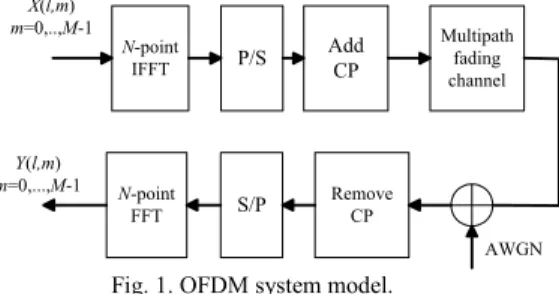
The baseband discrete-time equivalent model of an OFDM system is shown in Fig. 1. The modulation symbols to be transmitted are first grouped into blocks of size M. Each

N-point IFFT Add CP Multipath fading channel tex t AWGN P/S S/P Remove_CP N-point FFT X(l,m) m=0,..,M-1 Y(l,m) m=0,...,M-1

Fig. 1. OFDM system model.

block is zero-padded and transformed to the time domain using the inverse discrete Fourier transform (IDFT) of size N, where M ≤ N. If M < N, some subcarriers are not loaded with data or pilot symbols, and these subcarriers are referred to as the virtual carriers (VC). The IDFT outputs are next parallel-to-serial converted, and a cyclic prefix (CP) is prepended to obtain the time-domain OFDM symbol. Denoting the m-th subsymbol of the l-th block as X(l,m) and the n-th time-domain sample (chip) of the l-th OFDM symbolas x(l,n), the discrete-time baseband-equivalent transmitted signal is given by

) ( ) ) ( , ( ) ( 1 0 T N L l N T t n xl n lN J n lN x =

∑

− − − ∏ _T − = , (1) where (_•)N is the modulo-N operator, J is the length of CP, NT

= N+J is the length of an OFDM symbol, L is the number of

transmitted OFDM symbols in a burst, and

   ≤ < = ∏ else N n n T NT _0, 0 , 1 ) ( . (2) The signal xt(•) is transmitted over a wireless channel

modeled as a multipath fading channel corrupted by AWGN. At the receiver, CP is first discarded. The result is then serial-to-parallel converted into blocks of N and transformed into the frequency domain using N-point DFT. Let Y(l, m),

m = 0, 1, …, M – 1, be the received subsymbol on the m-th

active subcarrier in the l-th OFDM symbol. Assuming that frequency and timing synchronization are ideal, and the memory J’ of the discrete-time equivalent CIR is no longer than J, the observation window for each OFDM symbol can be suitably positioned such that

Y(l) = A(l)X(l)+ N(l), (3) where Y(l) = [Y(l,0),..,Y(l,M-1)]T _{and X(l) =}

transmitted OFDM symbols

,

N(l) is a zero-mean white Gaussian random vector with

[

]

_   = = else , , ) ( ) ( 2 0 I N Nl j l j E H σ M _{, (4)}

and A(l) is the M×M channel gain matrix. Assuming that the

channel remains approximately unchanged during one OFDM symbol interval, A(l) is a diagonal matrix whose diagonal entries are the frequency-domain gains at active subcarrier frequencies, and can be obtained by taking the

N-point DFT of [h(l,0),…,h(l, N–1)]T_{, where h(l, •) is the}

discrete-time equivalent CIR encountered by the l-th OFDM symbol.

III. OFDM CHANNEL ESTIMATIONBY KALMAN FILTERING

Let H(l) be an M×1 vector whose m-th component is the

m-th diagonal entry of A(l). The purpose of channel estimation is to find an accurate estimate for H(•) based on the observations Y(•). In order to use the Kalman algorithm for channel estimation, the channel H(•) is approximated as a first-order autoregressive process as follows. Assuming that the wireless channel is a Gaussian wide-sense stationary uncorrelated scattering (GWSSUS) channel with uniformly distributed angle of arrival [9], we have

[

+

]

=_ _≠= j i j i T f J P j l h i l h E i m , 0 ), 2 ( ) , 1 ( ) , ( * 0 π (5)

where Pi = E[|h(l, i)|2], fm is the maximum Doppler shift

frequency [9], T is the OFDM symbol interval, and J0(•) is

the modified Bessel function of the first kind with index 0. As a result, we have

E[H(l)HH_{(l+1)] =} H

mT f

J₀(2_π )WPW , (6) where P is an N×N diagonal matrix whose i-th diagonal entry is Pi and W is an M×N partial DFT matrix obtained from an

N×N DFT matrix by deleting the rows corresponding to the VC. The approximate first-order AR model can be derived from (6) by solving the Yule-Walker equations. The result is given by [8]

H(l+1) = F(l+1,l)H(l) + v(l), (7) where F(l+1,l) = F =J0(2πfmKT)WPWH in which K is a

constant computed according to various model matching criteria [8], and v(l) is a zero-mean vector random process that satisfies    ≠ = = + 0 , 0 , )] ( ) ( [ m m m l l E H 0 V v v , (8) where V =

(

)

H mKT f J (2 ) )WPW 1 ( 2 0 π − .

Given the AR model in (7), the well-known Kalman recursions can be used for estimating H(•). The Kalman estimator equations are given by [7]

1 2 _] ) ( ) 1 , ( ) ( )[ ( ) 1 , ( ) ( =FK − C C K − C + I− Gl ll H l l ll H l σ (9) ) ( ˆ ) ( ) ( ) (l Y l C l H l α = − (10) ) ( ) ( ) ( ˆ ) 1 ( ˆ _{l FHl Gl α l} H + = + (11) ) 1 , ( ) ( ) ( ) 1 , ( ) (_{l =Kll− −F}−1_GlClKll− K (12) V F FK K_(l+_1,l)= _(l) H+ ₍₁₃₎ FEQ Delay

Kalman Channel Estimator

) ( ˆ l H ) 1 ( ˆ _l+ H ) ( ˆ l X ) (l Y ) (l X Slicer

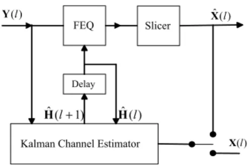
Fig. 2. OFDM receiver structure with Kalman channel estimator with initial conditions

0 H Hˆ(1)=E[ (1)]= (14) and H H E E E H H H H WPW K(1,0)= [( (1)− [ (1)])( (1)− [ (1)]) ]= , (15) where C(l) is an M×M diagonal matrix whose i-th diagonal element is X(l,i). It should be noted that the Kalman channel estimator operates in a decision-directed mode, i.e., past decisions are used in C(l) whenever the actual transmitted symbol X(l) is unavailable. The structure of an OFDM receiver with Kalman channel estimator after N-point FFT processing is shown in Fig. 2.

IV. LOW-COMPLEXITY KALMAN RECURSIONS FOR OFDM The complexity of the Kalman channel estimator can be greatly reduced when a circular constellation, e.g., phase shift keying (PSK), is used. To see this, we first factorize K(1,0) using eigenvalue decomposition (EVD) so that

K(1,0) = UD(1)UH_{, (16)}

where D(1) is an M×M diagonal matrix whose diagonal entries are the eigenvalues of K(1,0) and U is an M×M unitary matrix whose columns are the normalized right eigenvectors of K(1,0). We next use mathematical induction to show that, for all l > 1, K(l, l-1) has the same set of normalized eigenvectors as K(1,0) when a circular constellation is used. Assume that for some l ≥ 1, K(l, l-1) has the same set of normalized eigenvectors as K(1,0), thus

K(l, l-1) = UD(l)UH_{, (17)}

where D(l) is a diagonal matrix whose diagonal entries are the eigenvalues of K(l, l-1). Substituting (17) into (9), we have

(

)

[

]

(

()

)

() ) ( ) 2 ( ) ( ) ( ) ( ) ( ) ( ) ( 1 0 1 l l l KT f J l l l l l l H H M m H H M H H C U I D UD C U I D U C C U FUD G 2 2 − − + = + = σ π σ ,(18) where we have assumed that C(l)CH_{(l) = I}

M because a

circular constellation is used. From (12) and (13), we have

[

I F G C

]

K F V

F

K_(l+_1,l)= − −1 _{(l) (l) (l,l}−₁₎ H +

. (19) Substituting (18) into (19) gives

(

)

(

D I

)

D U F V FU V F U D I D D I FU K H H + + = +     _{− +} = + − − ) ( ) ( ) ( ) ( ) ( ) , 1 ( 1 2 2 1 2 l l l l l l l M M M σ σ σ , (20)

and from the initial condition in (15) and the definitions of V and F, we have

(

)

(

)

H m mKT J f KT f J K UD U V 1 (2 ) (1,0) 1 (2 )2 (1) 0 2 0 π = − π − = . (21) Thus H l l l UD U K( +1, )= ( +1) , (22) where

(

)

(

1 (2 )

)

(1) ) ( ) ( ) 2 ( ) 1 ( 2 0 1 2 2 0 2 D D I D D KT f J l l KT f J l m M m π σ π σ − + + = + − _{. (23)}

It can be seen from (23) that D(l+1) is also a diagonal matrix, thus from (22) that K(l+1, l) also has the same set of normalized eigenvectors as K(1,0). Therefore, by the principle of mathematical induction, we conclude that K(l,l-1) has the same set of normalized eigenvectors as K(1,0) for all l > 1.

Finally, substituting (18) in (11), we have

(

)

_   _{+ +} = + = + − ) ( ) ( ) ( ˆ ) 2 ( ) ( ) ( ) ( ˆ ) 1 ( ˆ 1 2 0 f KT l l l l l J l l l l H H M m H UD( )D( ) I U C α α G H F H σ π (24)

where α(l) is the innovations defined in (10). Since D(l) is a diagonal matrix, it is much simpler to update and store D(l) according to (23) than to propagate K(l,l-1) using the Riccati equations in (12) and (13) and compute G(l) by (9). From (23), for l=1,2…., the i-th diagonal entry of D(l) is given by

) 1 ( ) ) 2 ( 1 ( ) ( ) ( ) 2 ( ) 1 ( 2 0 2 2 2 0 i m i i m i J f KT l l KT f J l π λ σ λ λ σ π λ + − + = + (25)

The resulting low-complexity Kalman estimator structures will be shown in the next section.

The performance of the Kalman channel estimator can also be computed using (25). Specifically, define the mean-square channel estimation error (MSE) for the active subcarriers at time l as ] | ) , ( ˆ ) , ( | [ ) ( 2 1 0

∑

₌− − = Γ M m m l H m l H E l (26)

Since the estimation error covariance matrix at time l is given by K(l,l-1), we have

(

)

[

]

_∑

− = = − = Γ 1 0 ) ( 1 , ) ( M m i l l l tr l K _λ (27) Furthermore, by letting l approach infinity in (25), we can see that the limiting values λi(∞) for the eigenvalues of

K(l,l – 1) satisfy λi(∞)2 + aiλi(∞) + bi = 0, (28) where

(

)

[

1 2

]

[

1 0

(

2

)

2

]

(1) 2 0 2 i m m i J f KT J f KT a =σ − π − − π λ (29) and

(

)

[

1 2 2

]

(1) 0 2 i m i J f KT b _{=−σ − π λ} . (30) Substituting λi(∞) into (27) gives the limiting value of the

MSE.

V. LOW-COMPLEXITY CHANNEL ESTIMATOR STRUCTURES According to (16), the matrices U and D(1) can be obtained by performing EVD on K(1,0) given in (15). Due to the different structures of U, implementation structures for

OFDM systems with and without VC are discussed separately in this section.

A. OFDM without VC

For OFDM without VC, we have M=N, thus W is the N×N DFT matrix. We can therefore choose U W

N

1

= and

D(1) = NP. Since multiplication by UH _{and U can be}

implemented using the IFFT and FFT algorithms for this case, the Kalman channel estimator in (24) can be implemented as Fig. 3. Note that although a total of J′ real additions, multiplications, and divisions are required to evaluate (25), for a given fm λi(l) can be pre-calculated and stored. The

computations at time l therefore only include N complex multiplications and N complex additions required for the computation of α(l), the FFT and IFFT operations, J′ real multiplications at the output of the IFFT, and N complex multiplications and N complex additions for updating Hˆ l(). The complexity of the estimator in Fig. 3 is thus proportional to N+Nlog2(N), as opposed to N3 in the standard Kalman

channel estimator shown in (9) to (15). B. OFDM with VC

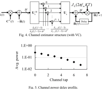
For OFDM systems with VC, we have M<N. Since the rank of P is J′, for every l D(l) has only J′ nonzero diagonal elements. The estimator in (24) can therefore be implemented as in Fig. 4, where λi(1) are the nonzero eigenvalues of

WPWH _{and U}

s is an M×J′ matrix whose i-th column is the

normalized right eigenvectors of WPWH_{corresponding to the}

eigenvalue λi(1). The matrix Us can be pre-computed and

stored for fixed P. Therefore the complexity of Fig. 4 can be similarly analyzed as Fig. 3 and shown to be proportional to N+NJ′.

It is interesting to note that the proposed channel estimator is similar to the time-domain LMS CIR estimator proposed in [6]. In particular, λi(l) in (25) plays the role of the adaptation

step-size of a variable step-size LMS CIR estimator. Equation (25) therefore provides a method for computing the “best” adaptation step-sizes for LMS CIR estimators for OFDM with circular constellation. In the proposed algorithm a different step-size is used for each CIR coefficient. The initial values of the step-sizes are determined from the power-delay profile, while the evolution of the step-sizes depends on the maximum Doppler shift frequency fm and

observation noise variance σ2_.

N-point FFT N-point IFFT 2 0 0 ) 1 , ( ) 1 , ( σ λ λ + − − l l l l ) ( ˆ l H ) 1 ( ˆ +l H N 1 '− J ) 2 ( 0 f KT J πm 2 1 ' 1 ' ) 1 , ( ) 1 , ( σ λλ − + − − − l l l l J J … Delay 0 1 2 0 0 ) (l Y ) (l H C −Hˆ l() N

U_s U_sH ) (l Y ) (l H C −Hˆ l() 2 0 0 ) 1 , ( ) 1 , ( σ λ λ + − − l l l l ) ( ˆ l H ) 1 ( ˆ +l H 1 '− J M ) 2 ( 0 f KT J πm 2 1 ' 1 ' ) 1 , ( ) 1 , ( σ λλ − + − − − l l l l J J … Delay 0 1 2 M

Fig. 4. Channel estimator structure (with VC).

1.E-02 1.E-01 1.E+00 0 2 4 6 8 Channel tap A vg. pow er

Fig. 5. Channel power delay profile. VI. SIMULATION RESULTS

The performance of the proposed Kalman channel estimators is evaluated by computer simulation for an OFDM system with 32 subcarriers (N=32). The CP length J is set to 8. Uncoded QPSK is used on active subcarriers. It is assumed that in each burst, a pilot OFDM symbol with known pilot subsymbols on all active subcarriers is followed by 99 data OFDM symbols. The number of active subcarriers is either M = 32 or M = 24.

The wireless channel is modeled as a GWSSUS multipath fading channel corrupted by AWGN. The discrete-time equivalent CIR is assumed to have 8 taps (J′=8) that are independent zero-mean complex Gaussian random variables, with the average power delay profile shown in Fig. 5. The modified Jakes’ model [9] with uniformly distributed arrival angles is used to simulate the time evolution of each channel tap within one burst. The channel is assumed to be uncorrelated across bursts.

At the receiver, perfect timing and frequency synchronization are assumed. The proposed channel estimation algorithms are then used in a decision-directed manner. A one-tap FEQ with coefficient computed from the estimated CFR is used for each subcarrier to undo the effects of the channel. The outputs of the FEQ are sent to the QPSK slicers for detection.

A. Learning Curves

Fig. 6 shows the MSE, defined in (27), as functions of OFDM symbol index l at Eb/N0=20dB, where Eb is the

transmitted energy per bit and N0/2 is the two-sided power

spectral density of the AWGN. Here the channel is assumed to be quasi-static, i.e., fm = 0. The curves labeled as

“LS” and “1D MMSE” are the MSE achieved by the linear LS and MMSE estimators, respectively, using only the pilot OFDM symbol, while “theoretical Kalman” is the MSE computed using (27). It can be seen that the simulated MSE matches very well with the theoretical values for this case. It can also be seen from Fig. 6 that the Kalman channel

estimator achieves the same MSE as the one-dimensional MMSE estimator after the first iteration. The MSE then continues to decays with symbol index while the receiver collects more observations and operates in a decision-directed mode. Because the channel is time-invariant, the MSE of the Kalman channel estimator approaches zero as l approaches infinity.

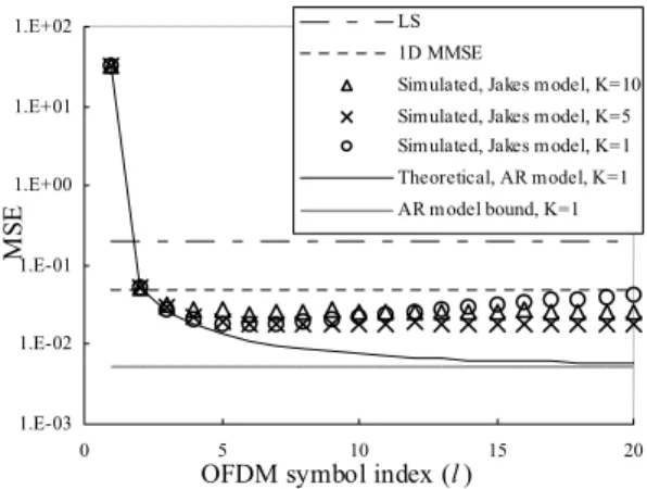
Fig. 7 is similar to Fig. 6, with the difference being that here fmT = 0.001. The model matching constant K for the

proposed Kalman estimator is set to 1, 5, and 10. The theoretical MSE (labeled as “Theoretical, AR model, K=1”) and its limiting value (labeled as “AR model bound, K=1”) are also computed and plotted for K = 1. These curves represent the MSE of the proposed estimator if the channel indeed follows a first-order AR model. It can be seen that because of the modeling mismatch between the Jakes’ and AR channel models, the simulated MSE of the Kalman estimators do not match the theoretical curve of the AR model. It can also be seen from the simulated MSE that K = 5 achieves good performance. The proposed channel estimator with K=1 does not have enough tracking capability and loses track of the channel after a few tens of OFDM symbols. On the other hand, large amount of excess noise is introduced when K = 10 is used in the Kalman estimator. Based on the results in Fig. 7, K = 5 is chosen for subsequent simulations.

B. Bit Error Rate Performance

The bit error rate (BER) performance of the proposed channel estimator is shown in Fig. 8 and 9 for OFDM with 32 active carriers as functions of Eb/N0. In Fig. 8, it is assumed

that no VC is used. The performance for quasi-static channels (fm = 0) and time-varying channels (fmT = 0.001) are plotted

using solid lines and dotted lines, respectively. For both types of channels, the LS and LMS channel estimators, as well as the “perfect” channel estimator are also simulated. It can be seen that for the quasi-static channel, LMS estimator that track each subchannel independently performs about 2dB worse than the proposed estimator that with frequency domain processing to exploit correlation between subchannels. Furthermore, for time-varying channels, the fixed channel estimators (LS) results in a BER floor. This floor is reduced somewhat by using the LMS adaptive channel estimator.However, the performance improvement is limited. A careful analysis of the simulation results shows that this is because the LMS estimator suffers from error propagation in the decision-directed mode. Finally, it is clear that the Kalman channel estimator almost achieves the same performance as the “perfect” channel estimator for both types of channels. It is interesting to note that the error propagation effect is not apparent in the Kalman estimator because feedback decisions from all active subcarriers are used jointly to adapt the CFR estimate for each active subchannel.

Fig. 9 is similar to Fig. 8, with the difference that out of the N=32 subcarriers, M = 24 are active and 8 are VC. Conclusions similar to Fig. 7 can also be drawn from this figure. However, because there are fewer observations in an

OFDM symbol, the effect of frequency-domain processing is 1.E-03 1.E-02 1.E-01 1.E+00 1.E+01 1.E+02 0 5 10 15 20

OFDM symbol index (l )

MS E LS 1D MMSE Simulated Kalman Theoretical Kalman

Fig.6. Learning curve of Kalman channel estimator for OFDM in a quasi-static channel (fm = 0), Eb/N0=20dB. 1.E-03 1.E-02 1.E-01 1.E+00 1.E+01 1.E+02 0 5 10 15 20

OFDM symbol index (l )

MS

E

LS 1D MMSE

Simulated, Jakes model, K=10 Simulated, Jakes model, K=5 Simulated, Jakes model, K=1 Theoretical, AR model, K=1 AR model bound, K=1

Fig. 7. Learning curves of Kalman channel estimator for OFDM in a fast fading channel (fmT=0.001), Eb/N0=20dB.

slightly worse than in OFDM without VC. Nevertheless, the proposed Kalman channel estimator still significantly outperforms other algorithms and almost achieves the same performance as the perfect channel estimator, because it exploits the information from the current and all past observations.

VII. CONCLUSION

Recursive MMSE channel estimators such as the Kalman channel estimator can be applied to OFDM systems. The Kalman channel estimator outperforms conventional adaptive and fixed channel estimators because it exploits prior knowledge about the statistics of the channel. However, the direct implementation of the Kalman equations leads to high receiver complexity, especially when the number of subcarriers is large. In this paper, low-complexity Kalman channel estimator structures are derived for OFDM systems with and without virtual carriers that use a circular constellation. It is shown that under the assumption of circular constellation, the Kalman channel estimator is very similar to the LMS channel estimator with variable stepsizes that are carefully initialized and adapted. Simulation results show that the proposed algorithm almost achieves the

performance of a perfect estimator. REFERENCES

[1] Hlaing Minn and Vijay K. Bhargava, “An Investigation into Time-Domain Approach for OFDM Channel Estimation,” IEEE

Transactions on broadcasting, vol. 46, no. 4, December 2000.

[2] A.A. Hutter, R. Hasholzner, J.S. Hammerschmidt, “Channel Estimation for Mobile OFDM Systems,” IEEE International Vehicular Technology

Conference, 1999.

[3] O. Edfors, M. Sandell, J.–J. van de Beek, S. K. Wilson, and P.O. Borjesson, “OFDM Channel Estimation by Singular Value Decomposition,” IEEE Transactions on Comm., vol. 46, no. 7, July 1998.

[4] D.N. Kalofonos, M. Stojanovic, and J. G. Proakis, “On the Performance of Adaptive MMSE Detectors for a MC-CDMA System in Fast Fading Rayleigh Channels”, IEEE PIMRC’98, vol . 3, pp. 1309-1313, September 1998.

[5] D. Schafhuber, G. Matz, and F. Hlawatsch, “Adaptive Prediction of Time-varying Channels for Coded OFDM Systems,” Proc. IEEE.

ICASSP-02, pp 2549-2552, May 2002.

[6] S. Haykin, Adaptive Filer Theory, 3rd _{Ed., Prentice Hall, 1996.}

[7] Christos Komninakis, Christina Fragouli, Ali H. Sayed, and Richard D. Wesel, “Multi-Input Multi-Output Fading Channel Tracking and Equalization Using Kalman Estimation,” IEEE Trans. on Signal

Processing, vol. 50, no. 5, May 2002.

[8] B. Bulumulla, S. A. Kassam, and S. S. Venkatesh, “An Adaptive Diversity Receiver for OFDM in Fading Channels,” ICC 98. vol. 3, pp. 1325-1329, Jun 1998.

[9] S.P. Dent, G.E. Bottomley, and T. Croft, Jakes fading model revisited,”

Electronics Letters, vol.29, no.13, pp.1162-1163, June 1993.

1.E-04 1.E-03 1.E-02 1.E-01 1.E+00 5 10 15 20 25 Eb/N0 (dB) Bit Er ro r Rate LS, fmT=0.001 LMS(stepsize=0.25),fmT=0.001 LS,fmT=0.0 LMS(stepsize=0.0625),fmT=0.0 Proposed Kalman,fmT=0.001 Proposed Kalman,fmT=0.0 Perfect Estimator

Fig. 8. Comparison of LS, LMS, and the proposed Kalman channel estimators for an OFDM system with 32 carriers and no VC.

1.E-04 1.E-03 1.E-02 1.E-01 1.E+00 5 10 15 20 25 Eb/N0 (dB) B it E rro r R at e LS, fmT=0.001 LMS(step=0.25), fmT=0.001 LS, fmT=0.0 LMS(step=0.0625), fmT=0.0 Proposed Kalman, fmT=0.001 Proposed Kalman, fmT=0.0 Perfect estimator

Fig. 9. Comparison of LS, LMS, and the proposed Kalman channel estimator for an OFDM system with 32 carriers and 8 VCs.