New Approach Combining Numerical Technique and Simulation for Analysis
of
Large Discrete Event Systems Based
on
Petri Nets
Ming-Hung L i n and Li-Chen
Fu
Dept.
of C o m p u t e r Science and I n f o r m a t i o n Engineering, National Taiwan University,Taipei, Taiwan,
R.0.C
E-mail:
[email protected] ABSTRACTIn this paper, me propose a new method that combines simulation and numerical techniques and directly in- tegrated using interval arithmetic techniques for the analysis of large discrete event systems. A system is first divided into several layers. Identifying subsys- tems that can be modeled in isolation solves a system for each layer. In each subsystem, the Markovian
as-
sumption allow-s us t o establish a set of linear equality constraints among the espectation of state variables in the Petri Nets, such as token numbers in the places. A pseudo random process is responsible for the timing of the model, event times are completely determined by simulation. Thus, linear equality constraints are com- puted according t o the pre-simulated event times, and it is possible t o know the probabilities of interactions between subsystems.1 I n t r o d u c t i o n
In this paper, a new analysis method for
a
discrete event system is introduced. For the analysis of a dis- crete event system, there are two different approaches can be used, simulation and numerical analysis. Jo-hannes (21 proposes mean value analysis for queueing
network models with intervals as input parameters. Shikharesh [3] presents robust bounds and throughput guarantees for closed multiclass queueing networks. The generalized stochastic Petri Net modules are used as basic building blocks to model and analyze complex manufacturing system (61. Matteo [8] describes ap- proximate mean value analysis for stochastic marked graphs. Zhen Liu [9] proposed performance analysis of stochastic timed Petri Nets using linear program- ming approach. Numerical analysis techniques and simulation both have their advantages and limitation. The idea of combining analytical/numerical techniques and simulation has been proposed several times. Pe- ter [l] presents a method for continuous time Markov chains. The basis of the method is the description of a continuous-time Markov chain as a set of commu- nicating processes. It also serves as a good tutorial paper. However, in practice, the probleni is usually the large size of state space and the model cannot be tlecornposed very cleanly.
In this paper, we propose a new niethotl that com-
m 2 Sub-system
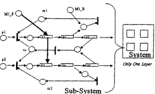
Figure 1: Hybrid model with only one layer
bines simulation and numerical techniques and directly integrated using interval arithmetic techniques for the analysis of large discrete event systems. A system is first divided into several layers. Identifying subsys- tems that can be modeled in isolation solves a system for each layer. In each subsystem, the Markovian as- sumption allows us t o establish a set of linear equality constraints among the expectation of state variables in the Petri Nets, such as token numbers in the places. A pseudo random process is responsible for the timing of the model, event times are completely determined by simulation. Thus, linear equality constraints are com- puted according t o the pre-simulated event times, and it is possible t o know the probabilities of interactions between subsystems. In this way, the state explosion problem of numerical analysis is avoided. It is still pos- sible to obtain more accurate results than with pure simulation.
The organization of this paper is as follows. Sec- tion 2 describes several types
of
combining model for performance analysis. Section 3 introduces aJF
queue- ing network that extends the framework of the origi- nal Jackson queueing network by adding event-driven in special queue. Section 4 describes a bounded Petri Net. Section 5 describes the development of integra- tion using interval arithmetic technique. Section 6 is conclusion.2 C o m b i n i n g Model
Hybrid model and Hierarchical model. The two model can bring together to solve the whole system. For ex- ample, in a flexible-manufacturing cell, there are two processes occurring in parallel. They both use a pool of common tools. Process 1 uses rnl machines and pro- cess 2 uses m 2 machines. Fig 1 represents the hybrid model of this system, where
p l number of process 1. p2 number of process 2.
m l available machines for process 1. m2 available machines for process 2. t o available tools.
Q1 number of process 1 a t input-buffer. Q3 number of process 2 at input-buffer.
Q2 number of process 1 at working-area and being
Q4 number of process 2 at working-area and being
Q5 number of process 1 at output-buffer. Q6 number of process 2 a t output-buffer.
M 1 E
number of failure machine 1.M 1 R
number of repaired machine 1. serviced.serviced.
.
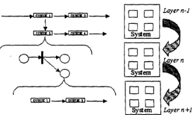
Notice that, transferring of a process (after service) from queue Q2,Q4,Q5 and QS, a token will be gen- erated. In this system, the machine 2 is the back-up machine for machine 1. When machine 1 becomes fail- ure, a new token triggers the instantaneous passage of a process from queue Q1 to Q3.On the other hand, in hierarchical model with mul- tiple layers, the system performance is calculated layer by layer. The Fig 2 represents this hierarchical model. The upper layer gives a coarse analysis and the lower layer gives a fine one.
A system is first divided into several layers. Iden-
tifying subsystems that can be modeled in isolation solves a system for each layer. 111 each subsystem, we establish a set of linear equality constraints among the expectation of state variables, such as token numbers in the places. -4 pseudo random process is responsible for the timing of the model, event times are completely determined by simulation. Thus, linear equality con- straints are computed according to the pre-simulated event times.The nest key goal is to know the interactions be- tween subsystems. In nest section, we proposed a J F
queueing m t w o r k that extends the framework of the original . J w h o n Quevein!l Network to add ability of event-driven.
/----/-
I I
System h y e r n + l
Figure 2: Hierarchical model with multiple layers
3
JF
Queueing NetworkThe
ModelThere are two types of queues, namely, joining queue and forking queue
.
The service time of joining queue is infinite. The service time of forking queue follow some probability distribution. The service time of forking queue is zero. Whena
customer enter a joining queue, the customer will receive no service from the server and will stay in queue for blocking. In our queueing network model, we allow work both t o be moved froma
queue t o another without service, and destroyed, un- der the effect of control customer which are either ex- ogenous, or generated by the ordinary customers after service. Before presenting our queueing model the nec- essary terminology is introduced. Let,C
= number of customer classes.I<
=
number of queues (resources modeled as queue-Nkc= number of class c E (1,. .
.
,
C)customers atVkc= mean number of visits made by a class c ordi-
&,=
mean number of external visits made by a classZk,=
mean number of external visits made by a classing centers or infinite server).
queue
k.
nary customer a t queue
k.
ordinary customer at queue
k.
control customer at queue
k.
Rkc= mean service demand rate per visit for a class c ordinary customer at queue
k
A customer(contro1 customer or ordinary cus- tomer)of class which leaves forking queue i (after finish service) goes to queue j as a customer of class I with probability p ( i , j ) ( k , l ) , it may depart from the network with probability P ( i ) ( k )
=
1-
E l
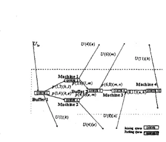
p ( i , j ) ( k , 1) . A customer (control customer or ordinary customer) of class k which leaves joining queue i (after finish service)Figure 3: A JF queueing model of a ordinary Jackson queueing network
Maddnt 1
Figure 4: A
JF
queueing model of share resource goes to queue j as a customer of class 1 with probability zero. The arriving control customer triggers the instan- taneous passage of a customer(contro1 customer or or- dinary customer) of class k from joining queue i to class 1 of some other queue j with probability q(i,j)(k,l).With probability Q ( i ) ( k ) = 1
-
C j
Cl
q ( i , j ) ( k , l ) , it forces a customer to leave the network. After trig- gering the instantaneous passage of a customer, the arriving control customer is destroyed. The arriving control customer triggers the instantaneous passage of a customer(contro1 customer or ordinary customer) ofclass IC
fromforking queue
i
to class1
of some other queue j with probability zero.When a customer(contro1 customer or ordinary cus- tomer) of class k which leaves forking queue i (after finish service)
,
it generates a new control customer from forking queuei
to class 1 of some other queuej with probability u ( i , j ) ( k , I). it may not generate
a. new control customer into the network with prob- ability U ( i ) ( k ) = 1
-
E, E,
~ ( i , j)(k,l) When a cus- tomer(coiitro1 customer or ordinary customer) of class k which leaves joining queue i (after finish service),
itFigure 5:
A
JF queueing model 0f.a production net- workgenerates a new control customer from joining queue i
to class 1 of some other queue j with probability zero.
Bounds on throughput
As usual the customers, in whom each queue is, define the operation of the system in terms of the execution of response cycles visited a certain number of times. Let,
Wk, = mean waiting time(pure delay) for a class c at
X,
= mean throughput for class c (cycle/second).Y, = mean cycle time for a single customer in class c
Hc =
h=
mean cycle rate fora
single customer in queue IC. (seconds)(seconds)
class c
The upper and lower bounds on the throughput for different customer classes in a open multiclass queueing network with a
FIFO
queueing discipline used a t each queue (queueing center) are presented in this section.The first type of upper bound ignores contention a t the queue and is termed the no contention upper bound. By ignoring the queueing delay a t every queue
k we obtain
k = l
for,each node of forking queue, we have tlk E {A-
,...,I<}
On the other hand, for each node of joining queue, we have V k E { I , . . .>I<'} 1 Ii c vkc = s k c
+
z k c+
, v k t C 1 p ( k ' , k ) ( c ' i c ) k' =U' c' = 1,
and form the little law we have.
Thus,.
Then,Figure 6: The basic bounded
TPPN
model are associated with the places. Denote by t j ( k ) the timeof
the kth firing of transition ti. Then, applying this notation leads t ot 4
(k)
=
max(min(p1+
t l(k),
p l+
tz(k)},
p 2+
t3(k-
2)) (3) There are recursive equations representing the firing time of the transitions. The real potential for this ap- proach is the ability t o draw on analogies with tradi- tional control theory. It is continue t o be proven that such analogies are not only with mathematical inter- est, and that in this approach can be extended t o a large model.However, uncertainties may be associated with
v k c b v k c '
hcWbc'
VbcRkc place. The uncertainties are based on the various rea---
I }Petri Net parameters such as number of tokens in a(1) 1 I\' Ck=llVkC x'c _<min{
ck=Ict
,(
Ii ' V&kC+
,
where b is the bottleneck queue for class c customers. L e m m a 1 Consider a closed system in which two cus- tomers, i in class a and j in class b, respectively, be at a FIFO queuek .
The probabilityP ( a ,
b) that customeri
upon arrival finds customer j in queue or service atk is upper bounded by P ( a , b )
5
min(1,R}
Proof : we omit the proof, which follows similar tech- nique [3].
T h e o r e m 1 Consider a closed multiclass queueing network corriposed of I< queues and
C
customer classes. If the customers arriving at a queue are served inFIFO
order, then,( 2 )
x:=L
N k cx ' c
L
z:=,
I,,E:=,
f i k , , ~ k , , min{l,Proof : we omit the proof, which follows similar tech- nique [3].
4 Bounded P e t r i Net
In order to cast the models of such systems in a lin- ear system-theoretic framework, minmax algebra is ap- plied to the Petri net models, and analogous concepts to transfer functions, input-output models, feedback, etc., are developed. This section will introduce some of these basic concepts.
Fig G represents the basic h l i n i m a that may be found in an\- TPPN model, where the time'delays di
sons. For example, exact values of firing time or exact numbers of arrival process are often unknown in some period of time. An external token visits made by a queueing network can be occur. On the other hand, a Petri net of another subsystem can also make external token visits. If the uncertainty is evaluated with the number of tokens in a place, then Eq 3 can be repre- sented as Eq
4.
Wherek-
5
k5 k + .
[ts(k-),td(k+)J = ma..{min([pl i- t l ( k ) - ,
Pl
+
t d k ) + l ,[PI+
t z ( k ) - - , p l + t*(k)+l},[p2 3- t3(k
-
2 ) - , p 2+
t3(k-
2)+]} (4)5 I n t e g r a t i o n Technique
A data type called interval, an object represents a real number locating between an upper and
a
lower bound which may vary during the lifetime of a computation. An interval x written as [x-,zc] which means that x lies between a lower bound x- and upper boundx+.
The main principle is that any operation whose argu- ments are intervals produces an interval that is guar- anteed t o contain all possible results of the operations in interval arithmetic;
Addition: [ x - , x + ]
+
[y-, U+] = [x-+
y-,z++
U+], Subtraction: [ x - , E + ] - [y-, g+] = [x--
y+, z+-
y-1:Division: [z-, z+]/[y-, y+]
=
[z-. r+]*
[l/y+, lly-1, In queueing network, the input parametersSkC
(mean number of visits made by a class c ordinary customer a t queuek)
and Z k c (mean number of exter- nal visits made by a class ordinary customer a t queuek)
can be evaluated with intervals. They can be re- placed by [Sic,s&]
and [S,,Szc]
respectively. For the queueing network bounds and Petri Yet bounds, the interval arithmetic can be used to calculate separate upper and lower bounds on each class throughput, giv- ing a rectangular box circumscribed around the feasible throughput region. Then, the next essential objective is to integrate those two different models. It is indi- cates that we must solve the interval parameters.In the queueing network, the external arrival tokens can be viewed as samples over a period At. The period may be short or long. In a number of instances the sample mean, or the sample mean and sample variance, are used to estimate the parameters of a hypothesized distribution [14].
If
the observations in a sample of size n areSI
,
.
. .
,
S,,
the sample mean-T
is defined byand the sample variance, S’, is defined by
On the other hand, we consider the marking m k ( p ) in Petri Xet, or mk for simplicity. Then, assuming that transition t j fires, j = 1 , .
. .
, 1 7 1mk+l(pi) = mk(pi)
+
O(tj,pi)-
I ( l j i , t j ) (7) for all places pi ,i=
1,.. . ,
11. Thus, marking m k ( p )be evaluated with intervals. The Eq 7 can be transfer into Eq 8 as following.
avoided. It is still possible to obtain more accurate results than with pure simulation.
Our
future work is development of throughput approximation technique based on interpolation or hIV.4 (2].The interval arith- metic, however, has so-called Jependency problem.
It is also as our future research.REFERENCES
[l] Peter Buchholz, “A New Approach Combining Simulation and Randomization for the Analysis of Large Continuous Time Markov Chains.”
,
ACM Tran. on Modeling and Computer Simulation. Vol. 8, No. 2, .4pril 1998, pp. 194-222.[2] Johannes Luthi and Gunter Haring, ”Alean \Blue Analysis for Queueing Network models ivith inter- vals as input parameters”
,
Performance Evalua- tion, Vol. 32, pp. 185-215, 1998.[3] Shikharesh RIajumdar and C. Murray Woodside, “Robust Bounds and Throughput Guarantees for Closed Multiclass Queueing Networks”, Perfor- mance Evaluation, Vol. 32, pp. 101-136, 1998. [4] Charles Knessl and Charles Tier, “Asymptotic Ap-
proximations and Bottleneck Analysis in Prod- uct Form Queueing Networks with Large Popula- tions”
,
Performance Evaluation, Vol. 33, pp. 219- 248, 1998.(51 K. Laevens and H. Bruneel, “Discrete-time hlulti- server Queues with Priorities”, Performance Eval- uation, Vol. 33, pp. 249-275, 1998.
[6] Robert Y. Al-Jaar and Alan A. Desrochers, “Per- formance Evaluation of Automated Manufacturing Systems Using Generalized Stochastic Petri Xets.”, IEEE Tran. on Robotics and Automation, Vol. 6, No. 6, Dec. 1990, pp. 621-638.
[7] Rossano Gaeta, “Efficient Discrete-Event Simula- tion of Colored Petri Nets.”, IEEE Tran. on
Soft-
ware Eng., Vol. 22, No. 9, Sep. 1996, pp. 629-639. [8] Matteo Sereno,
‘‘
Approximate Mean Value Xnal-ysis for Stochastic Marked Graphs.”, IEEE Tran.
In Petri Net, the arrival external tokens can be redis- tributed from the interval irlput of queueing network. Using Quantile-Quantile Plots technique[l4], the redis- tributed problem can be solved.
[91 Zhen Liu, “perfom~ance Analysis of Stochastic Timed Petri Sets Using Linear Programming -\p-
proach.”, IEEE Tran. on Software Eng., Vol. 24, NO. 11, NOV. 1998, pp. 1014-1030.
6 Conclusion
The present work introduces a new method that com- Ijines siitiulation ancl nurnerical techniques and directly integrated using interval arithmetic techniques for the analysis of large discrete event SySteIlis. In this way, the state explosion problem of numerical analysis is
[lo] Alan A. Desrochers and R.obert
Y.
AI-Jaar, ’.-\p- plication of Petri Nets in hIanufacturing Systems: hlodeling, Control, and Performance Analysis.”, IEEE Press.[ l l ] Ng Cllee Hock, ‘‘Queueing $Iodeling Fundamen- tals.”, John IC‘iley Sons Press.
[12] Leonard Kleinrock, “Queueing Systems Volume 1
[13] Leonard Kleinrock, “Queueing Systems Volume 2
: Computer Applications
.”,
John Wileyt3
SonsPress.
[14] Jerry Banks, John S. Carson, and Barry
L. Nel-
son, “Discrete-Event System Simulation.”, Prentice Hall International, Inc. Press.