A Versatile Copula and Its Application to Risk Measures

全文

(1)International Journal of Business and Economics, 2010, Vol. 9, No. 3, 213-231. A Versatile Copula and Its Application to Risk Measures Jeungbo Shim* Department of Business Administration, Illinois Wesleyan University, U.S.A. Eun-Joo Lee Department of Mathematics, Millikin University, U.S.A. Seung-Hwan Lee Department of Mathematics and Computer Science, Illinois Wesleyan University, U.S.A.. Abstract This paper proposes a copula that has versatile properties. We apply grouped t and versatile t copulas to estimate Value at Risk and expected shortfall using a sample of firms in the US property-liability insurance industry. We perform goodness-of-fit tests to assess the adequacy of the copula models selected. We find that a versatile copula is effective in estimating dependence structures of non-homogeneous multivariate risks. Key words: dependence structure; versatility; grouped t copula; value at risk JEL classification: C00; C13. 1. Introduction The financial markets have evolved dramatically over time, and financial firms are expanding their range of financial services, leading to a large discrepancy between the reality of the business today and its regulation. Recently, European Union (EU) financial supervisory authorities have developed the new regulatory capital requirement known as Solvency II for the insurance industry. The new regulatory framework would fix deficiencies in the current risk-based capital system and introduce more risk-sensitive and sophisticated solvency requirements in which insurers should take into account all types of risk to which they are exposed. The regulatory capital requirement obliges insurers to hold an amount of capital adequate to the amount of risk that individual firms are taking. To fully capture the level of risks inherent in the insurer’s asset and liability portfolios, one has to understand the. Received July 20, 2010, revised November 22, 2010, accepted December 3, 2010. * Correspondence to: Department of Business Administration, Illinois Wesleyan University, P.O. Box 2900, Bloomington, IL 61702, U.S.A. E-mail: jshim@iwu.edu. We would like to thank the editors and two anonymous reviewers for their helpful comments and suggestions..

(2) 214. International Journal of Business and Economics. importance of measuring dependence structure among different risk factors. The traditional method of measuring portfolio risks is based on the assumption, among other assumptions, that financial asset returns follow a multivariate normal distribution. However, recent studies show that dependence structure between assets returns tend to be nonlinear (e.g., Longin and Solnik, 2001; Trivedi and Zimmer, 2009). Thus, the assumption of Gaussian dependence is likely to underestimate the actual risks if return distributions exhibit tails that are fatter than those implied by normal distributions. Recently, copulas have become popular in modeling multivariate dependencies in the finance, risk management, and insurance literature (e.g., Frees and Valdez, 1998; Li, 2000; Embrechts et al., 2002; Ane and Kharoubi, 2003; Nelsen, 2006). In particular, the t copula is widely used in practice due to its ability to capture extreme tail dependence and its flexibility in terms of simulation and calibration (Embrechts et al., 2002; Demarta and McNeil, 2005). Mashal and Zeevi (2002) find that international equity market indices exhibit extremal behavior in a statistically significant manner and t dependence structure is superior to the Gaussian, correlation-based, dependence structure in representing extreme co-movements between financial assets. Breymann et al. (2003) show that the t copula provides a better empirically fit to high-density financial return data. There are several studies that explore the impact of the dependence structure between risks on the capital requirement using t copula functions. Tang and Valdez (2006) investigate the sensitivities of the capital requirement to the choice of the t copula using data from an Australian insurance company that writes multiple lines of businesses. Based on the class of elliptical copulas, such as Gaussian, t , and Cauchy, Shim et al. (2010) examine how different dependence structures between insurance underwriting risk and market risk have a substantial impact on the insurer’s total required economic capital for a sample of US property-liability insurance firms. Daul et al. (2003) suggest an extended model of the standard t copula, which is called the grouped t copula. The grouped t copula is suitable to describe the dependence structure for a mixture of different types of risk factors because it incorporates the dependence structure of non-homogeneous risk factors. In the grouped t copula, risk factors of similar type are grouped and each component group selects its own t copula with possibly different degrees of freedom, allowing for different levels of tail dependence in each component group. The grouped t copulas might be appropriate to describe the dependence structure in an insurance setting, where different types of risk factors, such as asset risk and liability risk, coexist. However, the grouped t copula has some drawbacks. For example, the grouped t copula requires an a priori choice of grouping among different types of risk factors. In certain cases where multiple risk factors of similar but different types coexist, it may not be clear about how to divide risk factors into distinctive groups. It may not be easy to divide risk factors into adequate sub-groups if there is no natural grouping (Luo and Shevchenko, 2010). The possibility of inadequate grouping may exist because grouping is determined by the researcher’s subjective decision. Inadequate choice of grouping could yield undesirable outcomes. In.

(3) Jeungbo Shim, Eun-Joo Lee, and Seung-Hwan Lee. 215. addition, additional computing cost is required to generate random return series separately on each component group for the calculation of risk measures. To remedy these problems, we propose a copula that has versatile properties, which we call the versatile copula. The versatility has been given a great deal of attention in the statistical literature, especially in the area of survival analysis (e.g., Lee, 2007). This versatile approach incorporates various dependencies of the component groups with one copula selected. The versatile t copula can be computationally more efficient for the purpose of calculating risk measures than the grouped t copula since one specific copula is applied simultaneously to all groups. Unlike the standard t copulas obtained under the assumption of homogeneous tail dependence, the versatile t copulas can be applicable to a various range of dependence structures because the versatile t copula is built using the degrees of freedom values used in the grouped t copula. Based on the combination of the degrees of freedom of t copulas selected from the grouped t copula, we construct versatile t copulas with the minimum, median, mean, and maximum degrees of freedom, and the middle of the degrees of freedom of Gaussian and Cauchy copulas. We apply these copula functions to model dependence structure between risks using data from the US property-liability insurance industry. We estimate risk measures value at risk (VaR) and expected shortfall (ES) under the grouped t and the versatile t copulas developed in this paper. VaR and ES are the most popular risk measures that summarize the levels of firm risk in a common dimension. To check the adequacy of the copula models selected, we perform goodness-of-fit tests using the method proposed by Genest and Rémillard (2008) and Genest et al. (2009). The paper is organized as follows. Section 2 provides a brief introduction of the multivariate t distribution and t copula. Section 3 discusses measures of linear dependence and characteristics of tail dependence of t copulas. Section 4 introduces the grouped t copula and develops versatile t copulas. Data, inputs used in the simulation algorithm, and the process of copula selection are described in Section 5. The estimation of VaR and ES and the procedures of the goodness-of-fit tests are also presented in Section 5. Section 6 concludes. 2. Model 2.1 Multivariate t Distribution We begin with a short introduction to the distribution for random vectors of correlated variables where each element has a univariate t distribution. This is the multivariate t distribution, which is a generalization of the univariate t distribution to two or more variables. The p -dimensional random vector X  ( X 1 ,..., X p ) is said to have a multivariate t distribution with  degrees of freedom, mean vector  , and p  p symmetric positive definite matrix  if the density is given by:.

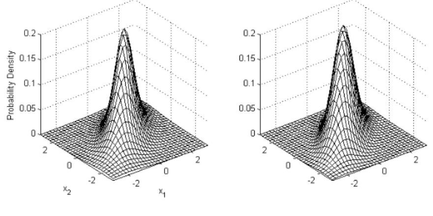
(4) 216. International Journal of Business and Economics   p     2  f ( x)    |  |1 / 2   ( ) p 2.  ( x   )  1 ( x   )  1     . . p 2. ,. (1). and it is denoted t p ( ,  , ) or tp,  , where  is interpreted as the shape parameter of the distribution of X . Note that the covariance of X is    2  and is only defined for   2 . See Johnson and Kotz (1973) for further discussions. It is well-known that the p -dimensional family of normal variance mixture models is equal in distribution to the product of a (scalar) random variable S  0 and a normal random vector Z  ( Z 1 ,..., Z p ) N p (0, ) plus  : d. X    SZ ,. (2). where S and Z are independent. For example, the multivariate t distribution with  degrees of freedom belongs to the class of multivariate normal variance mixture distribution if: S.  W. ,. where W has a chi-squared distribution with  degrees of freedom. Let f1 and f 2 be the marginal distribution functions of x1 and x2 , respectively. When p  2 and with the identity covariance matrix, the multivariate t distribution in (1) becomes f ( x1 , x2 )  f ( x1 ) f ( x2 ) .. Figure 1 shows the probability density of this bivariate t distribution with the identity covariance matrix where two variables are independent and identically distributed. Figure 2 displays the probability densities of the bivariate t distribution where the covariance matrix is chosen such that the correlation matrix between two random variables, X 1 and X 2 , is:. 1.    21. 12 .  1 0.7  .  1  0.7 1 . The correlation coefficient is a measure of the strength of relationship of two variables. In this situation, two variables are positively correlated, having a linear trend. Figure 2 shows that the bivariate t distribution when the correlation coefficient is radially symmetric. In summary, the multivariate t distribution not only shares many tractable properties of the multivariate normal distribution but also enables modeling of multivariate extremes that take non-normal dependencies..

(5) Jeungbo Shim, Eun-Joo Lee, and Seung-Hwan Lee. 217. Figure 1. Bivariate t Density Function with Identity Covariance and   5 (left) or   20 (right). Figure 2. Bivariate t Density Function with   0.7 and   5 (left) or   20 (right). 2.2 The t Copula A copula, expressed as C , is a p -dimensional distribution function on [0, 1] p with standard uniform marginal distributions. If F1 ,, Fp are univariate distribution functions, then C ( F1 ( x1 ), , Fp ( x p )) represents a multivariate distribution function with margins F1 , , Fp and is a joint probability distribution of random vectors with uniform marginal distributions. Sklar’s theorem (Nelson, 2006) states that every multivariate distribution function F can be written as. F ( x1 ,..., x p )  C ( F1 ( x1 ),..., Fp ( x p )) ,. (3).

(6) 218. International Journal of Business and Economics. for some copula C . The copula C is uniquely determined on [0, 1] p for F with absolutely continuous margins. Conversely, if C is a copula and F1 , , Fp are marginal distribution functions, then the distribution F given by (3) is a joint distribution function with F1 , , Fp . This implies that any copula C can be used to join univariate distributions to create a multivariate distribution function with margins. Let the random vector X  ( X 1 , , X p ) ' have marginal distribution functions that are continuous and strictly increasing. A unique copula function of their joint distribution can be extracted from a multivariate distribution function F from (3) by calculating: C (u1 ,..., u p )  F ( F11 (u1 ),..., Fp1 (u p )) ,. where F11 ,..., Fp1 are inverses of F1 ,..., Fp and are referred to as the quantile functions of the margins. The copula of F , C , can be thought of as the distribution function of componentwise transformations of the random vector X , and it remains invariant under strictly increasing transformations of its components. This is an appealing feature of copula over the correlation coefficient. Elliptical copulas are generally defined as copulas of elliptical distributions (Embrecht et al., 2003; Demnarta and McNeil, 2005). An example is the t copula. The t copula is useful when data do not take normal distributions and tend to have marginal distributions with heavier tails. The t copula of X given by (2) is derived from the multivariate t distribution defined in (1) and has the following representation: Ct ,  (u1 ,..., u p )  tp,  (t1 (u1 ),..., t1 (u p )) . 1 t1 ( u1 ) t ( u p ).   . . .   p     2    |  |1 / 2   ( ) p 2.  ( x   )  1 ( x   )  1     . . p 2. dx1    dx p ,. where t1 denotes the quantile function of a univariate t distribution and the parameter  controls the heaviness of the tails. As    , the t copula approaches the Gaussian copula, which is based on multivariate normal distribution. The useful property of the copula is its invariance under strictly increasing transformations of the margins. When the correlation matrix  is used in the integral, the copula of t p ( ,  , ) is identical to t p ( , 0,  ) , where the copula of t p ( , 0,  ) is:. Ct , (u1 ,..., u p ) . t1 ( u1 ). t1 ( u p ). . .   .   p  p     x  1 x  2  2  1   dx1    dx p .     |  |1 / 2   ( ) p  2. In the bivariate case, the copula expression can be written as:. (4).

(7) Jeungbo Shim, Eun-Joo Lee, and Seung-Hwan Lee. C ,  (u1 , u 2 )  t. t1 ( u1 ) t1 ( u2 ).  . . .  s 2  2 12 st  t 2  1    (1  122 )  2 (1  122 )  1. 219.  2. . 2. ds dt ,. where 12  12 11  22 is the usual correlation coefficient of the bivariate t distribution if   2 . The simulation of the t copula, Ct , R , is easily implemented. Equation (2) provides an algorithm for generating a multivariate t distributed random vector X and returning a vector U  (t ( X 1 ),..., t ( X p )) , where t denotes the distribution function of a univariate t . Any univariate marginal distributions can be imposed over a t copula. For example, if we combine several margins such as gamma, lognormal, and logistic using a t copula with   2 , we can generate a random vector from a multivariate distribution with gamma, lognormal, and logistic margins. This is termed a meta t distribution function (Embrechts et al., 2002; Fang et al., 2002). Of course, this includes the case of univariate t distribution margins with different degrees of parameters. 3. Dependence Structure 3.1 Linear and Rank Correlation. Linear correlation is a measure of linear dependence. Let X 1 and X 1 be random variables with finite variances. The linear correlation coefficient is:. . Cov( X 1 , X 2 ).  1 2. ,. where Cov( X 1 , X 2 )  E ( X 1 X 2 )  E ( X 1 ) E ( X 2 ) and  1 and  2 are the standard deviations of X 1 and X 2 , respectively. The popularity of linear correlation stems from its simple calculation and its naturalness as a measure of dependence in elliptical distributions such as the multivariate normal and the multivariate t distributions. However, linear correlation has some deficiencies. For example, linear correlation is not invariant under nonlinear strictly increasing transformations and is not even defined in the case of t distribution with   2 , which is a heavy-tailed distribution (Embrechts et al., 2002). An alternative dependence measure for non-elliptical distributions is Kendall’s rank correlation named Kendall’s tau. Kendall’s tau is a measure of dependence based on concordance. In some cases the concordance between extreme (tail) values of random variables is of interest. For example, one may be interested in the probability of the event that price changes in gold and oil exceed (or fall below) given levels (Trivedi and Zimmer, 2009). This requires a measure of dependence for lower and upper tails of the distribution, rather than a linear correlation. Kendall’s tau is given by (Embrechts et al., 2002; Nelson, 2006):.

(8) 220. International Journal of Business and Economics 1 1.  ( X 1 , X 2 )  4  C (u1 , u2 ) dC (u1 , u2 )  1 . 0 0. The above equation implies that Kendall’s tau depends only on copula C and not on the margins of X 1 and X 2 . Note that this is the expected value of the random variable C (u1 , u 2 ) , where u1 and u 2 are uniform random variables on (0, 1) with joint distribution C . Recall that  is the usual linear correlation matrix in (4). This  can be estimated by a robust linear correlation estimator. The main advantage of using Kendall’s tau is that it is invariant under monotonic transformations of the variables for a random vector. Thus, an estimate of  in (4) is obtained from the following representation:.  ( X1, X 2 ) . 2. . arcsin  .. For a proof, refer to Lindskog et al. (2003) and Fang et al. (2002). The t copulas considered here incorporate an estimate of  using the above relationship. 3.2 Tail Dependence. Tail dependence relates to the level of dependence that may exist in the upper or lower tails of the multivariate distribution. The coefficient of tail dependence is expressed as the limiting conditional probability of joint quantile exceedances. Specifically, for a pair of random variables, X 1 and X 2 , the coefficient of upper tail dependence is:. U  lim P( X 2  F21 (q) | X 1  F11 (q)) , q 1 provided the limit exists, and the coefficient of lower tail dependence is:. L  lim P ( X 2  F21 (q) | X 1  F11 (q )) , q 0  provided the limit exists. See Embrechts et al. (2003) for details on these expressions. For the family of elliptical copulas where distributions are symmetric, the two measures U and L coincide and are denoted  . If X 1 and X 2 have the t copula Ct ,P , the coefficient of tail dependence is given by:.   2t 1 (   1 1  . 1  ) ,. where  is the off-diagonal element of P . Based on this formula, Embrechts et al. (2002) calculate the coefficients of tail dependence for various values of  and  . Table 1 presents their results, which illustrate varying degrees of tail dependence with the t copula. The t copula shows asymptotic dependence in the upper tail even for negative and zero correlations. The value of the coefficient for the t copula is positive and is zero for the Gaussian copula (   ). Note that the strength of tail.

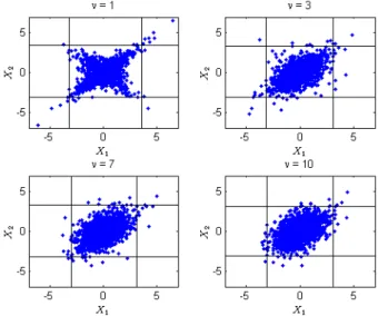
(9) Jeungbo Shim, Eun-Joo Lee, and Seung-Hwan Lee. 221. dependence increases as  decreases and values of correlation increase. Table 1. Coefficient of Tail Dependence of t Copula (Embrechts et al., 2002).    .   0.5.  0.   0.5.   0.9.  1. 2. 0.06. 0.18. 0.39. 0.72. 1. 4. 0.01. 0.08. 0.25. 0.63. 1.  10. 0.00. 0.01. 0.08. 0.46. 1. . 0.00. 0.00. 0.00. 0.00. 1. The t copulas have an interesting property that generates a different level of extreme values according to the degrees of freedom, although they have the same marginal distributions and the same rank correlation between variables. Figure 3 shows a scatterplot of 2000 simulations of random variables using t copulas with v  1 , 3, 7, and 10 degrees of freedom. All plots have the same rank correlation between variables ( 12  0.5 ) and the same margins ( t10 ). Vertical and horizontal lines mark the 0.005 and 0.995 quantiles of simulated distributions. Figure 3 clearly demonstrates that there is stronger evidence of upper and lower tail dependence as the degrees of freedom decreases. The form of tail dependence is not pronounced in the scatterplot with   10 compared to the plots of   1 and   3 . However, more pairs of joint extreme value observations are produced in the upper-right and lower-left quadrants of the scatterplot with   1 . This result implies that the dependence structure of multivariate distributions may not be well defined only by their marginal distributions and their correlations. Figure 3. Scatterplots of 2000 Simulations of Random Variables Using t Copulas with 12  0.5.

(10) 222. International Journal of Business and Economics. 4. Grouped t Copulas and Versatile t Copulas d. Let X  ( X 1 ,..., X p ) be given by X  S Z with  , where S and Z are defined in Section 2.1. Recall that by Sklar’s theorem the copula of X can be written as:. Ct ,  (u )  tp,  (t1 (u1 ),..., t1 (u p )) , where   { ij } for i, j  1,..., p ,  ij   ij  ii  jj , and tp,  is the distribution of Z W  , where W ~ 2 and Z ~ N p (0,  ) are independent. The tp,  is the multivariate t distribution function and t denotes the usual univariate t distribution function. Let F1 ,..., Fp be a continuous and strictly increasing distribution function. Then we obtain a t copula with margins F1 ,..., Fp :. Y  ( F11 (t ( X 1 )),..., Fp1 (t ( X p )) .. (5). As mentioned in Section 2.2, the distribution of Y is referred to as the meta t distribution, and it has a t distribution if and only if F1 ,..., Fp are univariate t distribution functions. The grouped t copula was proposed by Daul et al. (2003). Let Z ~ N p (0,  ) and divide the variable X indexed by 1,  , p into m subgroups of sizes d1 ,..., d m such that d1    d m  p and write: X  ( X 1 ,..., X m ) ,. where X 1  ( S1 Z 1 ,..., S1 Z d ) 1. . X m  (S m Z d. m 1. 1. ,..., S m Z p ) .. Note that X k , k  1,..., m , has an d k -dimensional t distribution with  k degrees of freedom. Accordingly, we obtain the following:. Y  ( F11 ( F1 (Y1 )),..., Fp1 ( Fp (Yp ))), , which is a generalization of the meta t distribution called the grouped t copula (Daul et al., 2003). Because the grouped t copula allows individual groups to possibly have different degrees of freedom parameters, each group may have a different level of tail dependence. As a special case, when m  1 and  1   , X has a meta t distribution, which is equal to (5) when    . The above procedures lead to a random variate:.

(11) Jeungbo Shim, Eun-Joo Lee, and Seung-Hwan Lee (t ( X 1 ),..., t ( X d ),, t ( X d d 1. 1. 1. m. 1. m 1. 1. ),..., t ( X p )) , m. 223 (6). where variables are partitioned into multiple subgroups and each subgroup has its own t copula with possibly different degrees of freedom. The grouped t copula may require various copulas to describe the distributional characteristic of individual subgroup variables. However, there is a possibility that poorly chosen groups may provide misleading information about the dependence structure of the variables considered since group classification is made by researcher’s judgment. Additional computing cost is also required to perform Monte Carlo simulation that generates random returns separately for each component group in a multi-group case. To overcome some of the drawbacks of the grouped t copula, we propose a versatile t copula in a nonparametric setting. Based on the combination of the degrees of freedom of t copulas that come from the grouped t copula, we first construct a versatile copula with the minimum of the degrees of freedom. Thus, (6) becomes: (t ( X 1 ),..., t ( X d ),  , t ( X d d min. 1. min. min. 1. m 1. 1. ),..., t ( X p )) , min. where  min  min( 1 ,..., v m ) . The Cauchy copula is a special case where the degrees of freedom is  min  1 . The versatile copula with minimum degrees of freedom is able to express extreme tail dependence and also may overstate the level of tail dependence for the given application. Second, we form the versatile copula with the maximum of the degrees of freedom. Then, (6) becomes: (t ( X 1 ),..., t ( X d ),  , t ( X d  d max. 1. max. max. 1. m 1. 1. ),..., t ( X p )) , max. where  max  max( 1 ,..., m ) . The tail dependence structure is less pronounced in this copula. As  max   , the copula approaches the Gaussian copula where it does not allow for extreme events to be dependent. For comparison, we also add three different types of combined copulas that still retain versatile properties. The first is the median of the degrees of freedom in the grouped t copula. Thus, (6) becomes: t ( X 1 ),..., t ( X d ),  , t ( X d  d med. med. 1. med. 1. m 1. 1. ),..., t ( X p )) , med. where  med is the median of the degrees of freedom in (6). Note that the median value is a robust measure of center, which is less affected by extreme values than the average. Thus, we expect the copula with the median of the degrees of freedom to be more versatile than the minimum- and maximum-based copulas. The average of the degrees of freedom is used to construct a new versatile copula: (t ( X 1 ),..., t ( X d ), , t ( X d  d avg. avg. 1. avg. 1. m 1. 1. ),..., t ( X p )) , avg. where  avg  ( 1     m ) m . Similar to the median, the average is a measure of center. The average value is more reliable than the median value when there are no extreme values in a sample. Finally, we propose a versatile copula that averages the.

(12) 224. International Journal of Business and Economics. number of the degrees of freedom of the Cauchy and Gaussian copulas. For simplicity of computation, we take the degrees of freedom for Gaussian copula to be 100 in this work. Thus, (6) becomes: (t ( X 1 ),..., t ( X d ),  , t ( X d  d CG. CG. 1. CG. 1. m 1. 1. ),..., t ( X p )) , CG. where  CG is the average value of 1 and 100. 5. An Application to Insurance Underwriting Risk and Asset Risk 5.1 Data, Marginal Distributions, and Correlations. We use data from the US property-liability insurance industry to apply the grouped t and versatile t copulas to the problem of describing the dependence structure between risk factors. We divide the risks of a property-liability insurer into two groups: underwriting risk and asset risk. It is reasonable to classify an insurer’s risks into these two groups for this study because its main profits (or losses) stem from underwriting (underwriting risk) and investment (asset risk) activities. Underwriting risk measures the risk that arises from under-estimating the liabilities from business already written or inadequately pricing current or prospective business. Underwriting risk is the largest portion of the risk-based capital charge for property-liability insurers. Asset risk is a measure of an asset’s default of principal or interest or fluctuation in market value as a result of changes in the market. We also consider four business lines to represent underwriting risk: special property (SP), commercial multiple peril (CMP), medical malpractice (MM), and workers compensation (WC). Underwriting risk is measured using quarterly industry-wide underwriting returns by line of insurance business. The underwriting return is defined as premiums written net of the present value of incurred losses for each quarter divided by premiums written for the quarter. We obtain the quarterly data on losses and premiums from the National Association of Insurance Commissioners. We include four categories of assets to characterize the insurer’s asset risk: stocks, mortgages, corporate bonds (CBond), and government bonds (GBond). The quarterly time series of returns are taken from a previous study (Shim et al., 2010) as proxies for asset risks: stocks (the total return on the S&P500 stock index), mortgages (Merrill Lynch mortgage-backed securities total return), CBonds (Moody’s corporate bond total return), and GBonds (Lehman Brothers intermediateterm total return). Summary statistics for the return series of underwriting and asset classes over the sample period 1991–2004 are presented in Table 2. To compare the performance of the grouped t and versatile t copulas, we also divide insurance underwriting and asset risks into four groups. Underwriting risk is divided into short-tail lines, which include SP and CMP and are more standardized with shorter loss payment duration, and long-tail lines, which include MM and WC and are more complex with longer loss payment duration. Asset risk is also categorized into two subgroups: stocks and mortgages are grouped together because have higher variability of returns (Browne et al., 2001) and CBonds and GBonds are.

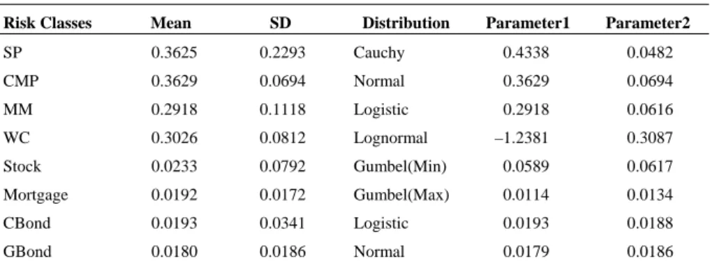
(13) Jeungbo Shim, Eun-Joo Lee, and Seung-Hwan Lee. 225. grouped together since they are less volatile investments. The marginal distributions of the underwriting and asset class returns and correlations between those classes are important inputs into the simulation algorithm using copulas. The distributional behavior of each business and asset class returns will differ with one another since the risks that each business and asset class covers vary to a great extent. Thus, we determine the best fitting marginal distribution on an individual business line and asset class basis using various graphical and numerical methods. Each of the selected distributions is fully specified by two parameters, and the maximum likelihood method is used to estimate these parameters. In Table 2, we present the appropriately selected marginal distribution and their estimated parameters given the data for each risk class. The correlation matrix between underwriting and asset portfolio classes is shown in Table 3. Table 2. Summary Statistics and Marginal Distributions Risk Classes. Mean. SD. Distribution. Parameter1. Parameter2. SP. 0.3625. 0.2293. CMP. 0.3629. 0.0694. Cauchy. 0.4338. 0.0482. Normal. 0.3629. MM. 0.2918. 0.1118. 0.0694. Logistic. 0.2918. 0.0616. WC. 0.3026. 0.0812. Lognormal. Stock. 0.0233. 0.0792. Gumbel(Min). –1.2381. 0.3087. 0.0589. 0.0617. Mortgage. 0.0192. 0.0172. CBond. 0.0193. 0.0341. Gumbel(Max). 0.0114. 0.0134. Logistic. 0.0193. GBond. 0.0180. 0.0186. 0.0188. Normal. 0.0179. 0.0186. Table 3. Estimated Correlation Matrix between Underwriting and Asset Classes CMP SP CMP MM. MM. WC. 0.6746. 0.0840. –0.1130. 0.1264. 0.4044. 0.2557. 0.3186. (<0.0001). (0.5746). (0.4495). (0.3973). (0.0048). (0.0828). (0.0291). 1.0000. Stock. Mortgage. CBond. GBond. 0.2621. 0.0837. 0.1983. 0.2877. 0.3838. 0.1509. (0.0751). (0.5761). (0.1816). (0.0499). (0.0077). (0.3113). 1.0000. 0.3219. 0.3933. 0.0932. 0.2574. 0.0163. (0.0274). (0.0062). (0.5331). (0.0807). (0.9136). 1.0000. 0.2702. –0.2469. –0.0986. –0.2496. (0.0662). (0.0944). (0.5096). (0.0907). 1.0000. –0.0908. 0.5570. –0.2833. (0.5441). (<0.0001). (0.0537). WC Stock Mortgage CBond. 1.0000. 0.1354. 0.9250. (0.3643). (<0.0001). 1.0000. –0.0146 (0.9222). Notes: P-values are in parentheses..

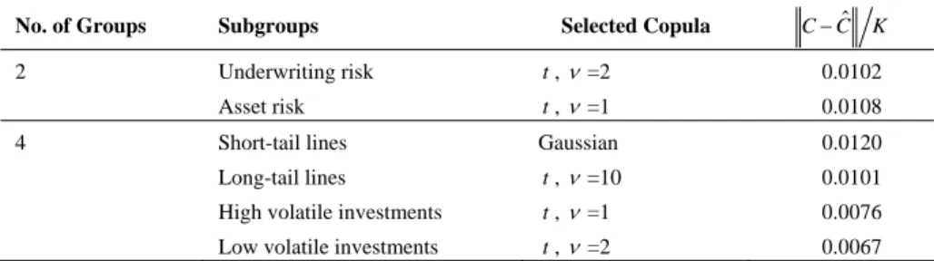
(14) 226. International Journal of Business and Economics. 5.2 Copula Selection. The selection of the component copula for each subgroup is an important issue in the study of the grouped t copula. In this section, we demonstrate how to choose an appropriate copula for our given subgroups using the method employed by Durreleman et al. (2000) and Palaro and Hotta (2006). Their procedures are based on the comparison of parametric and nonparametric values of a copula. For the nonparametric values, we use an empirical copula which is close to the theoretical copula when the sample size is large. The best copula is selected in such a way that the distance between the theoretical and empirical copulas is minimized. This method is generalized to high dimensions of our application data. Similar to the usual empirical distribution functions that assign equal probability to each observation in a sample, we define the empirical copula function for a random sample X 1, j ,... X n , j , j  1,..., K , from a multivariate distribution:  j  1 K  j C  1 ,..., n    I ( X 1, j  X 1,( j ) ,..., X n , j  X n ,( j ) ) , K  K j 1 K 1. n. where I is the indicator function and X i ,( j ) , i  1,...n , j  1,..., K , denote the ji th order statistic of the i th variable. The sum of the indicator function over j indicates the number of observations in a sample when the indicator function is 1. The best copula is chosen as the one that minimizes the distance between the theoretical copula ( C ) and the empirical copula ( Cˆ ). As a numerical measure of the distance, the L2 -norm criterion is given by (Durrleman et al., 2000): i. 1. 2 2 K K jn  ˆ  j1 j n    j1  ˆ C  C    C  , ,   C  , ,  .  j j K K  K K   1. n. We determine the appropriate component copulas for subgroups in the grouped t copula using the above formula. As discussed in Section 5.1, our application data are divided into two groups—underwriting risk and asset risk—and further divided into subgroups, namely short-tail lines, long-tail lines, high volatile investments and low volatile investments. The results in Table 4 show that t copulas with 2 and 1 degrees of freedom best fits the underwriting risk and asset risk factors, respectively. Similarly, the Gaussian and t copulas with 10, 1, and 2 degrees of freedom are selected to appropriately represent the dependence structure of short-tail lines, longtail lines, high volatile investments, and low volatile investments, respectively. 5.3 Value at Risk and Expected Shortfall. VaR is the most popular risk measure in recent financial risk management. VaR is the maximum likely loss from holding a portfolio over some target period at a specified confidence level (Crouhy et al., 2000). For instance, if a portfolio has a.

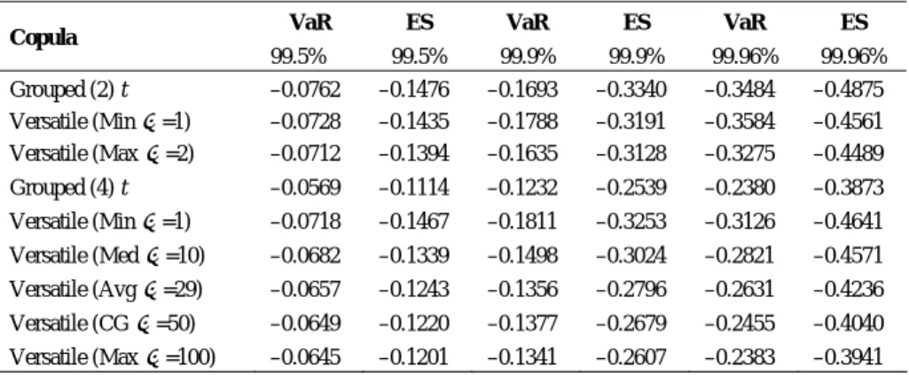
(15) Jeungbo Shim, Eun-Joo Lee, and Seung-Hwan Lee. 227. VaR of $5 million at the 99% confidence level, VaR then is the cutoff loss such that the probability of experiencing loss greater than $5 million is less than 1% over a given time period. VaR summarizes all risks of current portfolio positions into a single number. This explains why VaR is a crucial tool for conveying risk information to senior management and shareholders (Jorion, 2006). We also measure the significant loss beyond the quantile point by using the expected shortfall (ES). ES tells us the average size of the loss in excess of the cutoff value. Table 4. Selected Copulas and Values of the Distances for Each Subgroup Subgroups. 2. Underwriting risk. t ,  =2. 0.0102. Asset risk. t ,  =1. 0.0108. Short-tail lines. Gaussian. 0.0120. Long-tail lines. t ,  =10. 0.0101. High volatile investments. t ,  =1. 0.0076. Low volatile investments. t ,  =2. 0.0067. 4. Selected Copula. C  Cˆ. No. of Groups. K. To estimate VaR and ES under the grouped t copulas and various subsets of versatile t copula functions, we simulate 500,000 observations of return series for each underwriting and asset class using the parameters of the marginal distributions and correlations as inputs for specifying the copulas. We aggregate the simulated returns of an individual business line and asset class using its weights to construct a portfolio distribution. The VaR measure is simply computed from the quantiles of the aggregated portfolio returns distribution and the ES is obtained by calculating the sample mean of the simulated values above the corresponding quantile. The results of VaR and ES estimated with the grouped (2) and (4) t copulas and various versatile t copulas are presented in Table 5. For comparison, three confidence levels (99.5%, 99.9%, and 99.96%) are selected. The VaR at the 99.5% confidence level is the risk measure required by Solvency II capital requirements, 99.9% is consistent with the Basel Committee on Banking Supervision, and 99.96% is the AA rating target. Since risk managers are concerned about negative returns, VaR and ES are evaluated at the lower tail of aggregated returns distribution. We immediately observe that there is a significant difference in the value of risk measures according to the type of copula model selected. Interestingly, the grouped (4) t copula provides consistently lower VaR and ES than the grouped (2) t copula, displaying a range of risk measures between 68.3% and 79.5%. It is also observed that versatile t copulas with minimum   1 and median   10 , which allow for high tail dependence, lead to higher risk measures than does versatile t copula with the maximum of degrees of freedom, which does not account for tail dependence, indicating that tail dependence is increasing as the degrees of freedom are decreasing in the sets of versatile t copulas. The results underscore the importance of choosing the appropriate dependence structure in modeling risk measures. The choice of the adequate versatile t copula is an important issue to ensure.

(16) 228. International Journal of Business and Economics. that tail dependences between portfolio risks are properly identified. We assume that it is reasonable to classify insurer risks into two groups in this sample. Thus, the results of grouped t copula with 2 groups can be used as a benchmark to compare the performance with the results of versatile t copulas. Judging from estimates of VaR and ES in Table 5, the versatile t copula with the minimum of degrees of freedom is an appropriate choice for our given application data. Table 5 demonstrates that the estimates of VaR and ES computed from the versatile t copula with the minimum of the degrees of freedom are consistently closest to those of the group t copula with 2 groups across all confidence levels for both grouped (2) and grouped (4) t cases. The results indicate that the performance of the versatile t copula selected is comparable to that of a benchmarked grouped t copula, or could be superior to that of the less correctly specified grouped t copula. Note that it is also possible that, as a special case, the similar results can be observed with the well-chosen standard t copula obtained under the assumption of homogeneous tail dependence. Table 5. Risk Measures of Aggregate Portfolio Returns Using Grouped t and Versatile t Copulas VaR. Copula. 99.5%. ES. VaR. ES. VaR. ES. 99.5%. 99.9%. 99.9%. 99.96%. 99.96%. Grouped (2) t Versatile (Min  =1) Versatile (Max  =2). –0.0762. –0.1476. –0.1693. –0.3340. –0.3484. –0.4875. –0.0728 –0.0712. –0.1435 –0.1394. –0.1788 –0.1635. –0.3191 –0.3128. –0.3584 –0.3275. –0.4561 –0.4489. Grouped (4) t. –0.0569. –0.1114. –0.1232. –0.2539. –0.2380. –0.3873. Versatile (Min  =1). –0.0718. –0.1467. –0.1811. –0.3253. –0.3126. –0.4641. Versatile (Med  =10). –0.0682. –0.1339. –0.1498. –0.3024. –0.2821. –0.4571. Versatile (Avg  =29). –0.0657. –0.1243. –0.1356. –0.2796. –0.2631. –0.4236. Versatile (CG  =50). –0.0649. –0.1220. –0.1377. –0.2679. –0.2455. –0.4040. Versatile (Max  =100). –0.0645. –0.1201. –0.1341. –0.2607. –0.2383. –0.3941. We also perform goodness-of-fit tests to assess the adequacy of the copula model selected. Specifically, the procedures are based on the distance of the empirical copula and the copula distribution proposed by Genest and Rémillard (2008) and Genest et al. (2009). Consider the Cramér-von Mises type statistic: Tn  n.  Cˆ  C  dCˆ , 2. [ 0 , 1]K. where Cˆ is the empirical copula defined in Section 5.2 and C is the assumed copula. The statistic, Tn , is used to assess the adequacy of the given model. A large value of Tn indicates model misspecification. In particular, a p -value can be used as a numerical measure of how well a copula model fits data, and we can determine which copula is better based on this p -value. The p -value is defined as P (Tn  t ) , where t is an observed value of Tn , and it can be approximated by the standard bootstrap method. Note that the lower the p -value, the less likely the fit is good..

(17) Jeungbo Shim, Eun-Joo Lee, and Seung-Hwan Lee. 229. The results show that p -values of the grouped t copula with 2 groups, the grouped t copula with 4 groups, and the versatile t copula with the minimum of degrees of freedom values are 0.6095, 0.2140, and 0.4760, respectively, indicating that these copula models cannot be rejected to describe the dependence structure of the given sample. In particular, the results are consistent with earlier findings that the performance of the versatile t copula with the minimum of the degrees of freedom is competitive with that of a benchmarked grouped (2) t copula or that the versatile t copula could outperform the grouped t copula that is imperfectly specified. It also shows that, although the grouped t copula with 4 groups fits our sample, its performance is inferior to the grouped t copula with 2 groups. 6. Conclusion. The theory of copulas has received much attention in modeling joint distributions because copulas provide a method of generating a multivariate joint distribution by combining the marginal distributions and the dependence structure between variables. The copula has become a useful tool in modeling multivariate dependencies since it allows a wide of range of dependence structure according to the choice of copula functions. The t copula is commonly used to capture the extreme tail dependence of homogeneous risk factors. The recent literature suggests a grouped t copula to take the dependence structure of non-homogeneous risk factors into account. The grouped t copula focuses on issues related to the breakdown of risk factors of similar type and specification of its component copula by group. The grouped t copula might be a natural choice to describe a range of dependence structures of different risk factors present in the financial institutions. However, it may be challenging to split risk factors into appropriate groups in practice. Inadequate grouping could lead to inaccurate assessment of portfolio risks. In this paper, we propose a versatile copula that can be applicable to any set of risk factors regardless of whether they possess homogeneous or non-homogeneous characteristics. Versatile copulas are constructed based on the degrees of freedom in the grouped t copula. Using a sample of US property-liability insurance firms, we estimate VaR and ES under the grouped t copula and the versatile t copula. We find that the performance of the versatile t copula with the minimum of the degrees of freedom is competitive with that of a benchmarked grouped t copula with 2 groups. We check the appropriateness of the copula models selected with a goodness-of-fit test, and the results strengthen our findings. Thus, the versatile t copula represents an alternative dependence measure that overcomes some downsides of the grouped t copula. References. Ane, T. and C. Kharoubi, (2003), “Dependence Structure and Risk Measure,” Journal of Business, 76, 411-438. Breymann, W., A. Dias, and P. Embrechts, (2003), “Dependence Structures for.

(18) 230. International Journal of Business and Economics. Multivariate High-Frequency Data in Finance,” Quantitative Finance, 3, 1-14. Browne, M. J., J. M. Carson, and R. E. Hoyt, (2001), “Dynamic Financial Models of Life Insurers,” North American Actuarial Journal, 5, 11-26. Crouhy, M., R. Mark, and D. Galai, (2000), Risk Management, McGraw-Hill Publication. Daul, S., E. D. Giorgi, F. Lindskog, and A. McNeil, (2003), “The Grouped t Copula with an Application to Credit Risk,” Risk, 16, 73-76. Demarta, S. and A. McNeil, (2005), “The t Copula and Related Copulas,” International Statistical Review, 73, 111-129. Durrleman, V., A. Nikeghbali, and T. Roncalli, (2000), “Which Copula is the Right One?” Working Paper. Embrechts, P., F. Lindskog, and A. McNeil, (2003), “Modelling Dependence with Copulas and Applications to Risk Management,” in Handbook of Heavy Tailed Distributions in Finance, S. T. Rachev ed., Elsevier, 329-384. Embrechts, P., A. McNeil, and D. Straumann, (2002), “Correlation and Dependence in Risk Management: Properties and Pitfalls,” in Risk Management: Value at Risk and Beyond, M. Dempster ed., Cambridge University Press, 176-223. Fang, H., K. Fang, and S. Kotz, (2002), “The Meta-Elliptical Distributions with Given Marginals,” Journal of Multivariate Analysis, 82, 1-16. Frees, E. and E. Valdez, (1998), “Understanding Relationship Using Copulas,” North American Actuarial Journal, 2, 1-25. Genest, C. and B. Rémillard, (2008), “Validity of the Parametric Bootstrap for Goodness-of-Fit Testing in Semiparametric Models,” Annales de l’Institut Henri Poincaré - Probabilités et Statistiques, 44, 1096-1127. Genest, C., B. Rémillard, and D. Beaudoin, (2009), “Goodness-of-Fit Tests for Copulas: A Review and a Power Study,” Insurance: Mathematics and Economics, 44, 199-213. Johnson, N. and S. Kotz, (1972), Continuous Multivariate Distributions, New York: Wiley Publication. Jorion, P., (2006), Value at Risk: The New Benchmark for Managing Financial Risk, 3rd edition, McGraw-Hill Publication. Lee, S., (2007), “On the Versatility of the Combination of the Weighted Log-Rank Statistics,” Computational Statistics and Data Analysis, 51, 6557-6564. Li, D., (2000), “On Default Correlation: A Copula Function Approach,” Journal of Fixed Income, 9, 43-54. Lindskog, F., A. McNeil, and U. Schmock, (2003), “A Note on Kendall’s Tau for Elliptical Distributions,” in Credit Risk: Measurement, Evaluation and Management, G. Bol, G. Nakhaeizadeh, S. Rachev, T. Ridder, and K.-H. Vollmer eds., Heidelberg: Physica-Verlag, 149-156. Longin, F. and B. Solnik, (2001), “Extreme Correlation of International Equity Markets,” Journal of Finance, 56, 649-676. Luo, X. and P. V. Shevchenko, (2010), “The t Copula with Multiple Parameters of Degrees of Freedom: Bivariate Characteristics and Application to Risk Management,” Quantitative Finance, 10, 1039-1054..

(19) Jeungbo Shim, Eun-Joo Lee, and Seung-Hwan Lee. 231. Mashal, R. and A. Zeevi, (2002), “Beyond Correlation: Extreme Co-Movements between Financial Assets,” Working Paper, Columbia University. Nelsen, R., (2006), An Introduction to Copulas, 2nd edition, New York: Springer. Palaro, H. P. and L. K. Hotta, (2006), “Using Conditional Copula to Estimate Value at Risk,” Journal of Data Science, 4, 93-115. Shim, J., S. Lee, and R. MacMinn, (2010), “Measuring Economic Capital: Value at Risk, Expected Tail Loss and Copula Approach,” Working Paper, 36th European Group of Risk and Insurance Economists Seminar. Tang, A. and E. A. Valdez, (2006), “Economic Capital and the Aggregation of Risks Using Copulas,” Working Paper, 28th International Congress of Actuaries. Trivedi, P. K. and D. M. Zimmer, (2009), “Pitfalls in Modelling Dependence Structures: Exploration with Copulas,” in The Methodology and Practice of Econometrics: A Festschrift in Honour of David F. Hendry, J. Castle and N. Shephard eds., Oxford University Press, 149-173..

(20)