DiffServ RED Evaluation with QoS Management for 3G Internet Applications

全文

(1)DiffServ RED Evaluation with QoS Management for 3G Internet Applications Tzu-Chieh Tsai+ Computer Science Department, National Chengchi University Taipei, Taiwan, ROC. [email protected]. Po-Cheng Yang Computer Science Department, National Chengchi University Taipei, Taiwan, ROC. [email protected] Abstract+. 1.Introduction. With the increasing commercial deployment of wireless networks, the issue of providing multiple services is becoming more and more important. So the concept of “Quality of Service (QoS)” is being widely discussed and implemented. In the 3G architecture, the UMTS has defined 4 kinds of service types to provide the appropriate QoS type for different requirements and different applications. Similarly, in order to provide QoS in the traditional IP network, we assume 3G networks will adopt DiffServ as the IP-backbone. In this paper, we proposed an efficient mapping from 3G services to DiffeServ PHB aggregates. We used queueing theory to estimate the delay and loss for different traffic types. By using the estimation, we proposed a homogeneous QoS mapping policy to achieve QoS requirements under efficient resource utilizations through the 2 different services. An Admission Policy with QoS mapping is suggested to assure QoS by compromising with little throughput degradation. Besides, we also propose the adaptation policy. This adaptation policy could dynamically adapt the RED queue based on the arrival traffic types. Thus, we perform the QoS management through the RED evaluations. The QoS management includes the mapping and adaptation. For further development, we may also use these models to estimate and propose other mapping policies such as profit based mapping.. +. Wireless communications and Internet have grown tremendously for the past decade, and will be converged for providing ubiquitous integrated services. The 2nd generation (2G) mobile communication system, which is widely operated now, is mainly used for transmitting voice. It is inefficient to support data service on Internet. In addition, the data rate is only 9.6Kbps, it is not sufficient to support some applications which require more bandwidth or throughput. So the 3G system[1,2] is developed. 3G wideband technology increases data rate, which is 384kbps in the normal or walk situation, 128kbps in the vehicle situation and 2Mbps in the fixed situation. In order to support real time services, e.g. voice, vedio, end-to-end QoS[3,4] is an important part of this evolution. In the specification of 3GPP (3 rd Generation Partnership Project), the UMTS[5] has defined the QoS architecture and 4 different services which can support different QoS requirements for different applications. Traffic. Example of App.. Conversational Voice,Video telephony Real time Streaming streaming video Web browsing, Interactive Real time control channel Background Down of files and mails. Table 1. UMTS Service Classes Corresponding author 1. Capacity reservation type Static Static Dynamic. Dynamic.

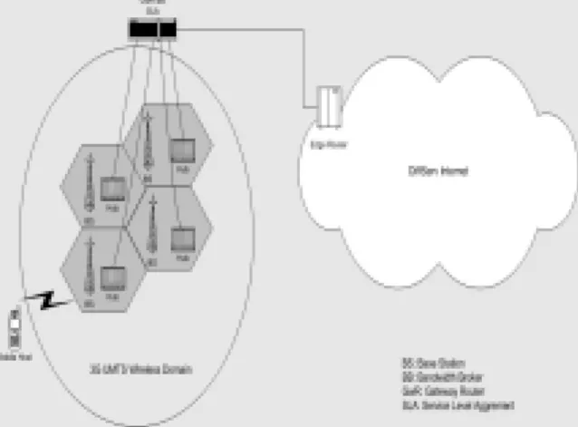
(2) policy. In Section 3, we propose the traffic model for estimate the delay and loss. This estimation is used for admission policy and mapping decision. Section 4 discusses the mapping issue and presents the homogeneous mapping policy. Finally in Section 5 we present a summary and point out our future research work.. The main distinguishing factor between these QoS classes is how delay sensitive the traffic is: Conversational class is meant for the traffic which is very delay sensitive while Background is the most delay insensitive traffic class. The QoS concepts are also taken into consideration in traditional IP network. IETF has two groups that are discussing the QoS on Internet, one is Integrated Service (IntServ)[6] and another is Differentiated Service (DiffServ)[7]. IntServ uses RSVP to reserve network resource to assure the service quality. And the DiffServ is between Best Effort and RSVP, which makes the network more scalable and resource usage more efficient. In differentiated service architecture[8,9], classification and conditioning functions of traffic are implemented only at boundary nodes entering the DiffServ Domain (called Ingress nodes). The ingress node marks the TOS (Type of Service) of each packet according to policy service provisioning. After being marked at the boundary node, packets are forwarded by appropriated PHB[10,11] on each node within the DS domain. Both boundary and interior nodes must be able to apply the appropriate PHB to packets based on the DS codepoint (DSCP). DiffServ has defined 3 different PHBs that are EF, AF and Best-Effort to achieve the different QoS requirements. In this paper, we assume DiffServ QoS model is adopted by IP backbone. Since the UMTS has defined 4 different service classes, all mobile applications will be marked as one of these classes. However mobile Internet sessions attempting to access to the DiffServ Domain will incur some problems. It is due to some gap between 3 DiffServ PHBs and 4 3G services. So, how to map the 3G services to DiffServ PHB aggregates will be a policy decision for the 3G operators. In this paper, we propose a mapping policy to achieve QoS requirements under efficient resource utilization through the 2 different domains. The rest of the paper is organized as follows: Section 2 presents the QoS framework and architecture for our mapping. 2.QoS and Mapping Framework This section we propose the QoS framework and the mapping interface for our mapping policy. The network architecture is shown as Figure 1. The GwR/BB is the gateway that is responsible for the call admission and resource allocation. Packets are marked as one of the UMTS service classes in UMTS Domain. These traffic classes provided by the 3G wireless networks should be mapped to the 3 DiffServ classes before they enter the DiffServ Domain. Thus, the GwR is the interface connecting to the DiffServ Internet backbone, where the SLA is negotiated to specify the resource allocation by the 3G operator to serve the aggregate traffic flowing into the gateway.. Figure 1. QoS Architecture And here we propose our mapping interface shown as Figure 2. This Mapping Interface should exist in the GwR and make the mapping decision for the 3G operator and thus for the call admission and resource allocation.. 2.

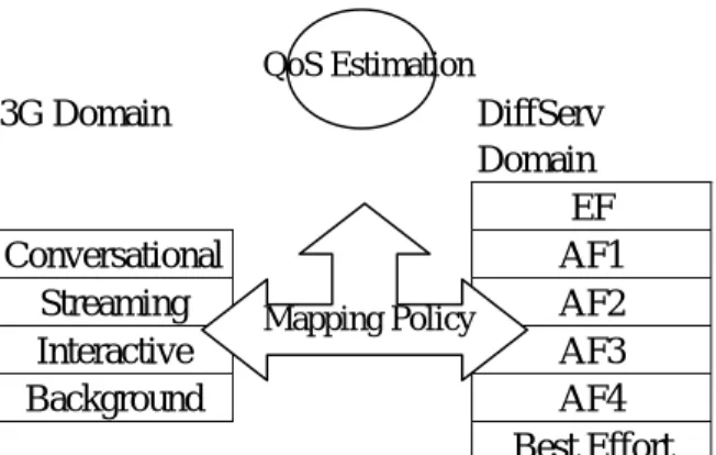
(3) queue is a kind of queue mechanism that the DiffServ suggest to implement the AF queue. These models can be used on the different traffic types, such as Poisson or CBR…etc. UMTS had defined 4 classes each belongs to different application types. Thus, our model can be used for the policy-maker to determine the delay and jitter of a given traffic. We consider a router with a queue size K. With the RED queue management scheme, arrival packets are dropped with a probability that is an increasing drop function of the average queue size. A typical drop function is defined by four RED parameters--minth , maxth , maxp , and w, where the w is usually a fixed and small parameter in RED. The average queue size is estimated using an exponential weighted moving average: avg_k = ( 1 – w ) avg_k + w k. QoS Estimation. 3G Domain. DiffServ Domain EF Conversational AF1 Streaming AF2 Mapping Policy Interactive AF3 Background AF4 Best Effort Figure 2. Mapping Interface The goal of mapping policy is to achieve QoS requirements (data rate, delay, jitter and loss) for both existing and new sessions. In other words, a new 3G session should be mapped to a certain PHB aggregate with acceptable QoS for all sessions within such an aggregate. Thus, we need to estimate the delay and loss for admitting this new session and for choosing the PHB aggregate. In section3 we introduce queueing delay model to calculate these. We also uses 3 traffic models for 4 3G UMTS services. As shown in Fig2.2, the Conversational and Streaming are mainly used on real-time applications that have higher delay requirements. Interactive and Background are used on traditional Internet applications such as WWW、E-mail or Telnet. From these attributes of each service, we model the Conversational and Streaming as CBR traffics; Interactive and Background as Poisson or Exponential On/Off traffics. So we model the queues as D/D/1、M/D/1 and Exponential On/Off models. In section 4, we propose the mapping policy for making the mapping decision. The mapping policy uses the queueing delay model to decide how to map a UMTS session to DiffServ Domain.. then the typical drop function is ： drop(avg_k) = 0 if avg_k < minth , drop(avg_k) = 1 if avg_k >= maxth otherwise, drop(avg_k) = max p ⋅ avg _ k − min th max th − min th. 3.1 RED with D/D/1/K model While the packet arrival is CBR （Constant Bit Rate）, then the queue model will become D/D/1/K. In this section we will discuss the delay and loss of the D/D/1/K queueing model.. 3.1.1 queueing delay and loss estimation Assume that the inter-arrival time is 1/λ, and the service time is 1/μ. Then we define the parameter n as： n =λ/μ. 3.Traffic Model with Queueing Delay Analysis. The n means the numbers of arrival packets in each service time. Here we take n≦2, because when the n bigger than 2, this system is thought. This Section we will analyze and evaluate the RED (Random Early Dection) queue[12,13] with different model. RED 3.

(4) super-overloading, and the arrival packets will be dropped with probability almost 1. So we take n≦2 as a reasonable and normal load. Then, by using Imbedded Markov Chain [14], we could get：. K. ∑ i =0. µ. ⋅ i + mean residual time (2). residual time as a half of service time, so the mean residual time is. pa,a-1 = [ drop(a – 1) ]. pa,a =Σi=1n drop(a)i-1 *(1-drop(a)) * drop(a+1). pa,a+1= Σi=1nΣj=in drop(a)i-1 *(1-drop(a))*.  λ−µ  loss _ probabilit y =  λ  0. drop(a + 1)j-i-1 (1-drop(a+1))*drop(a + 2)n-j The pa,b is one-step transition probability, i.e. the probability that a departure packet sees “b” packets in system given that the previous departure packet sees “a” packets in system. The transition probability matrix P is as. , when λ < µ. Compare with NS Now we consider the case of multiple flows entering into the same D/D/1/K queue. For simplicity again, here we still view the aggregated arrival traffic as deterministic. That is, the load will be:.    0 p21 p22 p23 0 ..... 0   0 0 p32 p33 p34 0.... 0  ..... ..... ..... ..... ..... ..........   ..... ..... ..... ..... ..... .......... (K+1)*( K+1) ..... ..... 0 ..... ..... 0. ρ =. ∑ m. λ. m. (4). µ. And we can use the above D/D/1/K RED model to estimate delay in the case of multiple flows. Next we give an example and compare it with ns2 results. Example: Suppose there are m CBR sources that enter the RED queue, the arrival rate are fromλ1 to λm and service rate is 5Mbps. The RED queue size is 40 with parameters minth=10, maxth=30 and maxp=0.1. The queue size is the same as maxth. The environment in NS2 is as follows:. then we can use this matrix to compute iteratively:. d ( j +1) = d ( j ) ⋅ P. , when λ > µ (3). 3.1.2 Multiple Flows Estimation and. follows: 0 0. 1 . 2µ. Then we consider the loss probability of this model. The loss probability of the RED queue will be:. n-I. p00 p01 p02 p10 p11 p12. 1. Here for simplicity we approximate the mean. n.     P=    . ri ⋅. (1). where d is probability vectors [d0, d1,…, dK], di is probability of seeing i packets in system when a packet departs the system. In this paper, we use a C-program to compute the stationary probability vector d. After computing d, we can estimate the system delay. In D/D/1/K model, we can let di = ri, where the ri represent the probability of seeing i packets when a new arrival enters the system. Then we can calculate the average system delay by:. S1 S2. λ1 λ2 . . . . λm. RED Queue. server. μ. Sm. Figure 3. NS2 Simulation Environment 4.

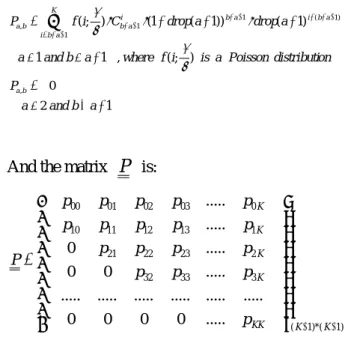
(5) Now we make a contrast between our models and ns2 from 1 flow to 5 flows. The results are shown as follows: No. of. Delay. Loss. Pa ,b =. K. ∑. i = b − a +1. λ µ. f (i; ) ⋅ C bi − a +1 ⋅ (1 − drop(a − 1)) b − a +1 ⋅ drop(a − 1) i − ( b − a +1). λ µ. ∀a > 1 and b > a − 1 , where f (i; ) is a Poisson distribution Pa ,b = 0. Difference. ∀a > 2 and b < a − 1. multiplexing flows 1. 2. NS. 0.02428 0.332 Delay < 1.7%. And the matrix P is:. D/D/1/K. 0.02388 0.333 Loss < 0.3%. NS. 0.02194 0.0904 Delay < 4%.     P=    . 0.090. Loss < 1%. NS. 0.021239 0.087. Delay <1 %. D/D/1/K. 0.02149 0.090. Loss < 4%. D/D/1/K 3. 4. 5. 0.0214. NS. 0.02169 0.0897 Delay < 0.1%. D/D/1/K. 0.02149 0.090 Loss < 0.3%. NS. 0.02187 0.0904 Delay < 1 %. D/D/1/K. 0.02149 0.090 Loss < 0.4 %. p 00. p01. p 02. p 03. ...... p0 K. p10 0. p11 p 21. p12 p 22. p13 p 23. ..... ...... p1K p2 K. 0. 0. p 32. p 33. ...... p3K. ...... ...... ...... ..... ...... ...... 0. 0. 0. 0. ...... p KK.          ( K +1)*( K +1). Again, we use equation (1) to compute d , and equation (2)、(3) to get the delay and loss.. Table 2. Comparison with D/D/1/K and NS2. 3.2.2 Comparing with NS Again, we make a contrast between the M/D/1/K model and NS2. The NS2 simulation environment is the same as D/D/1/K (Figure 3) besides the arrival type becoming Poission.. 3.2 RED with M/D/1/K model This section we discuss the M/D/1/K model where the arrival is Poisson and service rate is deterministic. Poisson is a general arrival type for many applications. And deterministic service rate can be used for the AF class of the DiffServ Domain. Because we use the Weighted Round Robin scheduler to serve the AF sub-classes (The RFC suggest we use 4 sub class for AF — AF1 to AF4), each service time of the queue of sub-class is deterministic.. Because arrival is Poisson, the multiple flows estimation can be easily modeled by simply summing up these Poisson arrivals. Then we still ma k e th e co n tr as t b e tw e e n NS an d th e M/D/1/Kmodel. No. of. Delay. Loss. Difference. multiplexing flows 1. 3.2.1 Queueing Delay and loss estimation Firstly, we have to compute one-step transition probability p a,b , the calculate scenario is the same as D/D/1/K model.. 2. 3. The p of M/D/1/K is as follows:. NS. 0.0239386. 0.36 Delay < 0.1%. M/D/1/K. 0.023943. 0.37. NS. 0.030063. 0.424 Delay < 0.5%. M/D/1/K. 0.03023. 0.428. Loss < 1%. NS. 0.0234149. 0.32. Delay < 2%. M/D/1/K. 0.023943. 0.37. Loss < 15%. Loss < 2%. Table 3. Comparison with M/D/1/K and NS2. 5.

(6) 3.3.2 Multi-Flow Estimation. 3.3 RED with Exponential ON/OFF. At the beginning, we analyze the case of multiple flows from two. So we suppose there are 2 exponential on/off traffic where the mean time of ON period is x1 and x2 , the mean time of OFF period is y1 and y2. The arrival rate during ON period is λ1 and λ2 . Then we firstly consider the probability that both exponential on/off traffics are during On period. Given source 1 is during On period, the probability of seeing source 2 during On period is: λ1 x2 × λ1 + λ 2 x2 + y2. Traffic This section we will discuss the traffic type—Exponential ON/OFF. This traffic type generates traffic according to an Exponential ON/OFF distribution. Packets are sent at a fixed rate during ON period, and no packets are sent during OFF period. Both ON and OFF periods are taken from an exponential distribution and packets are constant size.. 3.3.1 Queueing Delay Estimation Because packets are sent at a fixed rate during ON period, we can take it as CBR traffic. Thus, we separate this case into 2 parts and analyze the 2 parts respectively. First part is the ON-period, we could use the D/D/1/K model to estimate the delay due to the characteristic of Exponential ON/OFF traffic. Second part is the OFF-period, we know that no packet is sent during OFF period, but, we have to consider the tail effect when system load is bigger than 1. For simplification, we assume that the buffer is exactly full when entering OFF period, and the average delay is the mean buffer size multiply the service time. This is the idle time compensation that compensates the delay caused by the remaining packets when entering OFF period. Suppose the mean time of ON period is x ms, the mean time of OFF period is y ms and arrival rate is λ during ON period, we can estimate the delay as:. Similarly, given source 2 is during On period, the probability of seeing source 1 during On period is : x1 λ2 × λ1 + λ 2 x1 + y1 So the probability that both flows are during On period is as follows: λ1 x2 λ2 x1 pboth _ on = × + × λ1 + λ2 x 2 + y 2 λ1 + λ2 x1 + y1 Next we consider the case that only one flow is during On period. Given source 1 is during On period, the probability of seeing source 2 during Off period is: λ1 y2 × p s 1 _ on = λ1 + λ 2 x2 + y2 Given source 2 is during On period, the probability of seeing source 1 during Off period is: y1 λ2 p s 2 _ on = × λ1 + λ 2 x1 + y1. x × avg _ ON _ delay + idle _ time _ compensati on x+ y. Similarly, due to the tail effect, we have to consider the idle time compensation. In the 2-flows case, the compensation will be: y1 y2 × × compensate d _ delay x1 + y1 x 2 + y 2. where the avg_ON_delay is estimated by D/D/1/K model with arrival rateλ and idle_time_compensation will be:. Where the compensated_delay is calculated by formula (5) Then the delay is estimated as follows: pboth _ on × d both _ on + p s1 _ on × d s1 _ on + p s 2 _ on × d s 2 _ on. , if load < 1 0 (5) =  mean buffer size× servicetime , if load > 1. + idle _ time _ compensation. 6.

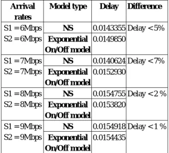
(7) influence of the mapping from 3G to DiffServ Domain.. dboth_on is the delay of both traffic during On period, it is calculated by using the D/D/1/K model with arrival rateλ1+λ2 ; ds1_on is the delay of only source 1 during On period and is calculated by using D/D/1/K model with arrival rateλ1; ds2_on is the delay of only source 2 during On period and is calculated by using D/D/1/K model with arrival rateλ2. Now, in order to make sure that our estimation is correct, we make a contrast between our model and ns2. Here we assume there are two Exponential On/Off flows entering one RED queue where the parameters are min th =10, max th =30 and maxp=0.1. The mean time of On period and Off period of each traffic are all the same—500ms. Then we list the result of the experiment as the following table:. 4.1 Homogeneous QoS Mapping In Section 3, we have proposed 3 different Queueing Model that are corresponding to different traffic types. Now we can use that model to implement the homogeneous mapping. Suppose there are 6 queues in the Ingress of DiffServ Domain, 1 for EF class, 4 for AF sub-classes (from AF1 to AF4) and 1 for Best-Effort. The schedular is the Weighted Round Robin, so each queue has a different service rate. μ1 EF μ2. Arrival Model type rates S1 = 6Mbps NS S2 = 6Mbps Exponential On/Off model S1 = 7Mbps NS S2 = 7Mbps Exponential On/Off model S1 = 8Mbps NS S2 = 8Mbps Exponential On/Off model S1 = 9Mbps NS S2 = 9Mbps Exponential On/Off model. Delay. AF1. Difference. 3G UMTS Services. 0.0143355 Delay < 5% 0.0149850. μ3 AF2. Server μ4. AF3 μ5. 0.0140624 Delay < 7% 0.0152930. AF4 μ6 BE. 0.0154755 Delay < 2 % 0.0153820. Figure 4. Mapping Architecture. 0.0154918 Delay < 1 % 0.0154435. EF is a kind of resource-reservation service class and the traffic type is usually CBR, so the queue model will be a D/D/1/K with FCFS queue. Packets are enqueued when the buffer has enough space and are dropped when the buffer is full. AF provides the relative QoS instead of absolute QoS. It means that AF1 will receive lower drop precedence than AF2 to AF4, and AF2 will receive lower drop precedence than AF3 and AF4. AF service class is implemented by some queueing mechanism to ensure the relative QoS. Here we use RED ( R a n d o m E a r ly D e t ec t i o n ) q u eu e i n g mechanism to implemen the 4 sub classes of AF. As we mentioned before, RED queue has 3 main parameters—minth, maxth and maxp. According to different consideration, AF1 to. Table 4. Comparison with Exponential On/Off traffics and NS2. 4.QoS mapping This section we will discuss the QoS mapping that is from 3G network to DiffServ Domain. The UMTS had defined 4 different service classes — Conversational, Streaming, Interactive and Background. Each class has its corresponding application and QoS requirements such as the Table 1. And the DiffServ domain define 3 different service classes that are EF, AF and BE respectively. We will then use the queueing model discussed in Section 3 to investigate the 7.

(8) have loose QoS requirement and the reservation type are dynamic (Table 1). We can easily map it to AF class without any resource-reservation. Here we let AF3 and AF4 be the corresponding queue to Interactive and Background. By using the M/D/1 model and Exponential On/Off model, we can estimate its delay and loss and use this information to perform the admission policy. So here we propose our admission policy for the QoS mapping as follows:. AF4 will have different parameter settings. Then the 4 sub classes of AF will have different service rate (μk, where the k is from 2 to 5 in Figure 4) and drop function. In order to make the homogeneous mapping, we implement the AF1 queue as the D/D/1/K model that the arrival traffic type is CBR; AF2 queue as the Exponential ON/OFF model that the arrival traffic type is Exponential On/Off; AF3 and AF4 queue as the M/D/1/K model that the arrival traffic type is Poisson. Then we model the AF queues as Table 5 AF. Traffic Type. AF1. CBR. AF2. CBR. AF3. Exponential On/Off. AF4. Poisson. If arrival traffic type is “Conversational” or “Streaming” then If EF bandwidth is available then Map this session to EF Elseif EF bandwidth is unavailable then Use D/D/1/K model to estimate the delay, loss and jitter of AF1 queue. Table 5. Homogeneous Queue Type. If the estimating QoS correspond to UMTS then. Last, the Best-Effort class can be modeled as M/G/1 model. The arrival traffic type is Poisson and has loose QoS requirement. The service rate is a general distribution because it varies depends on the situation of other queue. When some AF queue are empty, the service rate of BE queue will be larger than that when most of the AF queues are busy.. Map this session to AF1 Elseif not corresponding Use D/D/1/K model to estimate the delay, loss and jitter of AF2 queue If the estimating QoS correspond to UMTS then Map this session to AF2. 4.2 Admission Policy for the QoS. Else Reject this session. mapping Now we consider the admission policy for the QoS mapping from UMTS service classes to DiffServ service classes. Because the Conversational and Streaming class have strict QoS requirement, we will map it to EF class if the remaining bandwidth is available. If the EF bandwidth is not available, we could also map it to AF1 or AF2 classes. But, we must use D/D/1/K model to estimate the delay and loss to make sure that this mapping will still conform to the QoS requirement of UMTS. Interactive and Background classes. If arrival traffic type is “Interactive” then Use M/D/1/K model to estimate the delay, loss and jitter of AF3 queue If the estimating QoS correspond to UMTS then Map this session to AF3 Else Use M/D/1/K model to estimate the delay, loss and jitter of AF4 queue 8.

(9) We let a simple mapping policy is that directly map the Conversational and Streaming to EF, Interactive to AF and Background to Best-Effort. This simple mapping (or we call it default mapping) is a straightforward mapping without QoS consideration. Thus, we make the contrast between the simple mapping and our homogeneous mapping policy.. If the estimating QoS correspond to UMTS then Map this session to AF4 Else Reject this session If arrival traffic type is “Background” then Use M/D/1/K model to estimate the delay, loss and jitter of AF4 queue If the estimating QoS correspond to. Throughput. UMTS then Map this session to AF4 Else Map this session to Best-Effort. 800 700 600 500 400 300 200 100 0. Conversational Streaming Interactive Background. Default Mapping. Homogeneous Mapping. Figure 5. Throughput comparison between 2. This session we make the simulation with our mapping policy. The simulation environment is that total bandwidth for Ingress is 40Mb, and the bandwidth distribution is EF—10Mb, AF—20Mb and Best-Effort for 10Mb. Here we suppose there are n1 Conversational traffics, n2 Streaming traffics, n3 Interactive traffics and n4 Background traffics. The QoS requirements of each service class are as table 5. mapping policies. 40 30 20 10 0. Conversational Homogeneous Mapping. Streaming Default Mapping. Delay (ms). 4.3 Simulation. Interactive Background. Figure 6. Delay comparison between 2 Delay. Rate Conversational 4~25 kbps Streaming. Delay. Reliability. mapping policies. Variation <150. <1 ms. <3%. ms. 32~384 <10 sec. <1 ms. <1%. Interactive. 4~13. <1 sec. <1 ms. <3%. Not. Not. ~0%. kbps Background. Not. Conversational Streaming Default Mapping. kbps. 0.6 0.5 0.4 0.3 0.2 0.1 0. Defined Defined Defined. Homogeneous Mapping. Data. Loss Probability. Service. Interactive Background. Figure 7. Delay comparison between 2 mapping. Table 6. QoS Requirement Parameters [18]. policies.. 9.

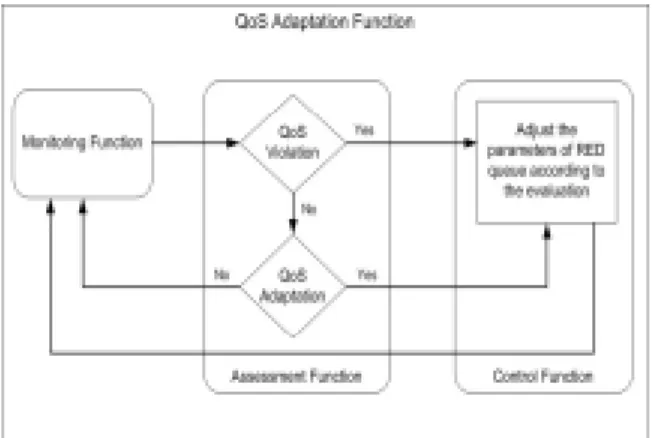
(10) From Figure 5 to 7, although the homogeneous mapping we proposed degrades the throughput, it extremely promotes the QoS for each service class. Thus, our mapping policy is based on the QoS achievement instead of throughput.. 5.QoS Adaptation In section 4, we have proposed the QoS admission policy for mapping and evaluate the performance of each queue model. A service provider should guarantee the service quality for all customers who have been admitted to the system. Thus, when the service provider’s system and network conditions are changing, service provider must be able to dynamically adapt the system in order to guarantee the system quality. In this section, we propose the QoS adaptation function and evaluate the influence of adaptation. Our adaptation is focus on the class adaptation instead of flow adaptation. Because DiffServ uses RED queue to implement the service provisioning, we could adapt the RED parameters to perform the QoS adaptation. The adaptation aspects could be delay or loss probability and this is a trade-off issue. Raising the loss probability could obtain better delay performance and increasing the max threshold could get lower loss probability but higher delay.. Figure 8. QoS adaptation functional description The QoS adaptation function can be processed as follows: Step 1: Initialization Step 2: Performance monitoring Step 3: Current state assessment a) If QoS violation occurs, then go to Step 4 b) If QoS Adaptation is required, then go to Step 4 c) Go to Step 2 Step 4: QoS adaptation a) Determine the parameters of RED queue b) Adjust the parameters according to the adaptation evaluation c) Go to Step 2 Next section we will propose the adaptation evaluation. The adaptation evaluation can be used for service provider to determine how to adjust the RED queue and the influence of changing those parameters.. 5.1 QoS Adaptation Function T h i s s ec t i o n we d e s cr i b e a Q o S adaptation function based on the proposed queue model. It is composed of a monitoring function, an assessment function, and a control function. It is shown as Figure 8. The monitoring function plays the role of monitoring the performance of the RED queue and network resource status. The assessment function decides whether a QoS violation occurs or QoS restoration is required. If required, the control function adjusts the parameters of the RED queue to guarantee the QoS of each queue.. 5.2 QoS Adaptation Evaluation Basically, RED queue uses 3 parameters that are maxth, minth, and maxp. Augmenting the value of max th could reduce the loss probability but increase the delay. So we firstly investigate the influence of changing the value of maxth.. 10.

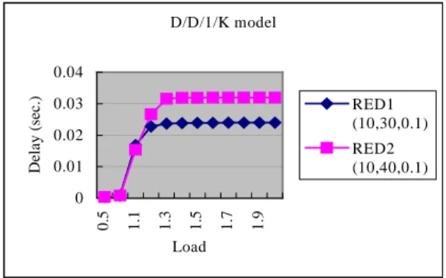
(11) improves 38% while the dropped packets just increase 2.4%. This is because raising the value of parameter maxp makes the number of early dropped packets increase. So this adaptation can be used to dynamically adjust the RED queue based on the different traffic types. For instance, if the arrival traffic type is Conversational or Streaming, which is more sensitive on the delay instead of loss, we could increase the parameter maxp to obtain better delay performance. Similarly, when the arrival traffic type is Background, we could greaten the maximum threshold—maxth to decrease the loss. By using this concept, we could define the QoS mapping as the following table:. D/D/1/K model. Delay (sec.). 0.04 0.03. RED1 (10,30,0.1). 0.02. RED2 (10,40,0.1). 0.01 1.9. 1.7. 1.5. 1.3. 1.1. 0.5. 0 Load. Figure 9. D/D/1/K model with different parameter of maxth Now we consider the situation of changing the value—maxp :. 0.03 0.025 0.02 0.015 0.01 0.005 0. Service Type. Parameter needed to be Adapted. RED1 (10,30,0.1). Conversational. Increase maxp. RED2 (10,30,0.2). Streaming. Increase maxp. Interactive. Decrease maxth and Increase maxth. Background. Decrease maxth and Increase maxth. 1.8. 1.5. 1.2. RED3 (10,30,0.3) 0.5. Delay (sec.). D/D/1/K model. Load. RED4 (10,30,0.4). Table 8. Adaptation Method. RED5 (10,30,0.5). Thus, our adaptation evaluation provides an efficient way to determine how to adjust the parameters of RED queues.. Figure 10. D/D/1/K model with different parameter of maxp. 6.Conclusions and Future Work. From these evaluation, we can see that when the system load is bigger than 1, adjusting the parameter of RED queue could get high performance of delay and the drop probability is not increase too much. For instance, we take a look at the D/D/1/K model with system load is 1.2. The variation of delay and loss are shown as Table 7. RED. RED2. While most of the work on Quality of Service has focused on specifying the service type and definition, our work addresses the issues for defining the mapping policy that performs the mapping between 2 different network domains which both has its own QoS definitions. The 2 different network domains we discuss here are 3G and DiffServ. UMTS had defined the 4 different QoS service classes for 3G and DiffServ had 3fundamental PHB types for implementing the QoS. In this paper, we firstly propose the traffic model for modeling the arrival traffic to estimate the QoS parameters—delay, loss and jitter. According to different traffic types, we propose different corresponding models that are D/D/1, M/D/1 and Exponential. Improvement. (10,30,0.1) (10,30,0.5) Avg. delay 0.022735 Drop Pkts. 10000. 0.013967. 38 %. 10024. 2.4 %. Table 7. Contrast between delay and loss In Table 7, we adjust the parameter maxp from 0.1 to 0.5, and the average delay 11.

(12) [7] S.Blake, “An Architecture for Differentiated Services”, RFC 2475, Dec 1998. [8] K.Nichols and S.Blake, “Differentiated Services Operational Model and Definitions”, Internet draft, Feb 1998. [9] Y.Bernet et.al. , “A Framework for Differentiated Services”, November 1998, Internet Draft. [10] J.Heinanen, “Assured Forwarding PHB Group”, RFC 2597, June 1999. [11] V. Jacobson, “An Expedited Forwarding PHB”, RFC 2598, June 1999. [12] Thomas Bonald, Martin May, “Analytic Evaluation of RED Performance”, IEEE INFOCOM 2000. [13] Sally Floyd and Van Jacobson, “Random Early Detection Gateways for Congestion Avoidance”, IEEE/ACM Transactions on Networking, Aug. 1993. [14] Leonard Kleinrock, “Queueing Systems”, Volume I :Theory, John Wiley&Sons. [15] Bain Engelhardt, “Introduction to Probability and Mathematical Statistics”, second edition, Duxbury. [16] Martin May, J.C.Bolot, Alain J.Marie and C.Diot, “Simple Performance Models of Differentiated Services Schemes for the Internet”, Proceedings of INFOCOM 99’, New York, March 1999. [17] B.Braden et al, “Recommendations on Queue Management and Congestion Avoidance in the Internet”, RFC 2309, April 1998. [18] “QoS Concept and Architecture”, 3GPP, TS 23.107 version 5.0.0.. On/Off models. Then from these models, we address the homogeneous mapping for admission policy. The homogeneous mapping policy estimates the delay and loss and decides how to map or reject. It promotes the QoS achievement but degrades the throughput. This mapping policy just provides the concept for performing the mapping based on different aspects. Future works will first focus on the heterogeneous mapping policy. This will cause the complicated situation for performing estimation and traffic modeling. Then we may also think about the QoS adaptation. The adaptation could be used to re-map the current session or adjust the bandwidth distribution for each service type. These issues are needed to research. And, we believe the mapping policy will make the network more efficient.. References [1] Juha Kalliokulju, “Quality of Service management functions in 3rd generation mobile telecommunication networks”, WCNC, IEEE 1999. Pp. 1283-1287. Vol.3. [2] Shaw-Kung Jong and Belka Kraimeche, “QoS Considerations on the Third Generation (3G) Wireless Systems”, in Academic/Industry Working Conference on Research Challenges, 2000, pp. 249-254. [3] Sanjoy Sen, Arun Arunachalam and Kalyan Basu, “A QoS Management Framework for 3G wireless networks”, in Wireless Communications and Networking Conference, IEEE 1999, WCNC, pp. 1273-1277, Vol.3. [4] “Technical Specification Group Services and System Aspects: QoS Concept”, 3GPP, TR 23.907, version 1.2.0. 1999. [5] “Enabling UMTS/Third Generation Services and Applications”, UMTS Forum Report No.11, Oct, 2000. [6] R.Braden, “Integrated Services in the Internet Architecture: an Overview”, RFC 1633, July 1994. 12.

(13)