An Enhanced Medium Access Control Protocol for Multi-Channel
Multi-Interface Wireless Mesh Networks
Fen-Cheng Yang, Michael Pan, and Sheng-De Wang
Department of Electrical Engineering
National Taiwan University, Taipei, Taiwan
Email: [email protected]
Abstract -
Multiple non-overlapping channels specified by the IEEE 802.11 wireless LAN standard can be used simultaneously to increase the aggregate bandwidth. However, multi-channel multi-interface protocols may incur a type of hidden terminal problems. The existing multi-channel multi-interface IEEE 802.11 Medium Access Control (MAC) protocols have room to be improved. In this paper, we propose an enhanced MAC protocol with a hybrid channel assignment strategy and a dynamic waiting time scheme for multi-channel multi-interface WMN to avoid the multi-channel hidden terminal problem. The proposed dynamic waiting time scheme assigns an appropriate waiting time for each channel by using the information of traffic loads to utilize the available bandwidth and reduce the end-to-end delay. From simulation results, we show that the proposed MAC protocol can increase system throughput and decrease the end-to-end delay.Keywords: Wireless Mesh Networks, Multiple
channels, Multiple interfaces, Multi-channel Hidden Terminal Problem, Waiting Time
1. Introduction
Wireless mesh networks (WMN) [1] is a kind of multi-hop wireless networks which are composed by mesh access points (APs). These mesh APs are like fixed routers, except that they are connected only by wireless links and have to forward packets that are received from neighbor nodes. The WMNs are connected to the Internet by some of nodes called mesh portals. In the IEEE 802.11 architecture, using WMNs to construct a wireless distributed system can decrease the links to wired networks and reduce lots of cost in constructing WLANs. Because of the reasons above, there are more and more WMNs constructed in commerce applications.
In multi-hop networks, due to the multiple times of forwarding overheads and hidden/exposed terminal problems [2][3], the available bandwidth might drop dramatically [4]. Jun et al. [5] show that for WMNs the throughput of each node decreases to O(1/n), where n is the numbers of nodes in the network. IEEE 802.11 standards [6] [7] provide several
non-overlapping frequency channels that could be used to communicate simultaneously within a neighborhood to increase throughputs. One interface with a multi-channel switching mechanism [8] [9][10][11] or [12] can be used to utilize all of the available bandwidth. When using a single interface to switch between multiple channels, it would spend some time, called the switch latency, to switch among the channels. Also, it may cause the multi-channel hidden terminal problem that will increase the probability of collision.
The most important issue in channel multi-interface architectures is how to effectively assign channels to interfaces. By effectively assigning channels to interfaces, we can decrease the interference between nodes and increase the total network capacity. In a node with a multi-channel multi-interface setup, every interface can just be assigned one specific channel and can only receive and transmit packets on that channel. Thus, interfaces have to be assigned the same channel to communicate to each other. A good channel assignment can effectively increase the number of simultaneously traffic flows, and reduce the interference caused by simultaneous transmissions between nodes. In [13], the authors classify the channel assignment schemes into three classes: the static channel assignment [12], the dynamic channel assignment [14], and the hybrid channel assignment [15][16][17][18]. In the static channel assignment, the channel was assigned to the interface for a long period of time, and the interface will not or rarely switch its channel. The dynamic channel assignment allows interfaces to switch among several channels to suit the requirements of communication at that time. In this situation, nodes should have a mechanism for negotiating the communication channel, which can be further classified into two classes: single rendezvous, multiple rendezvous [19]. The hybrid channel assignment scheme combines the advantages of the static and the dynamic channel assignment.
The proposed scheme belongs to the hybrid architecture and is based on the MAC protocol of HMCP [18][13] and HMCMP [17]. The MAC protocol in HMCP can be divided into two parts: channel assignments and channel switching mechanisms. HMCP assumes that every node has two half duplex
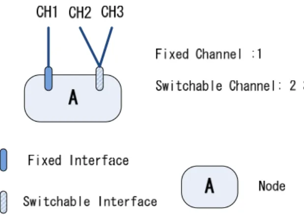
interfaces. One of the interfaces is called the fixed interface, and the other interface called the switchable interface. The fixed interface uses the static channel assignment to select its channel. The primary goal of the fixed interface is to solve the rendezvous problem. If nodes want to communicate with others, they just have to switch their interface to the receiver’s fixed channel and they can communicate in that channel without pre-negotiation. The switchable interface uses the dynamic channel assignment to dynamically switch its channel to fit the requirement of the traffic load.
Fig. 1 illustrates an example of a node with a switchable interface and a fixed interface.
Fig. 1 Example of Switchable Channel
In order to reduce the number of channel switches, HMCP uses the same number of queues to map channels. If there has a new packet to be transmitted, it only has to insert the packet into the queue corresponding to the channel of the destination node, as shown in Fig. 2. Thus, in an interval of time, the switchable interface is forced to transmit the packets in the same channel without switching between channels so as to reduce the effect of switching delay. The fixed interface only serves the queue corresponding to the fixed channel, and the other queues are served by the switchable interface.
Fig. 2 Illustration of Queues associated with 3 channels and 2 interfaces
The staying time on each channel must be carefully assigned. The maximum period of the switchable interface to serve a queue is called MaxSwitchTime. Using a shorter period increases the switching overhead, while using a longer period may cause starvation of other channels and more end-to-end
delay. The switchable interface always switches to the channel that has oldest packets in the queue. It switches to a new channel only when the other queues are not empty and one of the following conditions holds:
(i). The queue of the current switchable channel is empty.
(ii). The switchable interface has been on the current channel for more than the MaxSwitchTime duration.
Due to the multi-channel hidden terminal problem, nodes have to set a period of waiting time after switching to a new channel to avoid collision. The period of waiting time is assigned as the maximal packet transmission time. The maximal packet transmission time can be calculated by using the formula below: SIFS ACK MaxPacket CTS RTS Total
T
T
T
T
T
T
=
+
+
+
+
3
×
where TRTS denotes the period of time required to transmit an RTS packet, TCTS is the time needed to transmit a CTS packet; TMaxPacket denotes the time required to transmit a maximal size packet, TACK is the time needed to transmit an ACK packet, and TSIFS is the time of waiting an SIFS period. However, even there is no ongoing communication, a node should wait a period of the maximal packet transmission time after every switching to a new channel.
Li et al [17] proposed HMCMP to improve the performance of HMCP by replacing the static staying time, MaxSwitchTime, with the dynamic staying time, and using a shorter waiting time to replace the maximal packet transmission time. HMCMP divides the MaxSwitchTime into two parts, as shown in Fig. 4. The first part is the fixed staying time. The fixed staying time should be minimized for every channel to utilize all channels and avoid spending most of the time on switching channels without transmitting packets. The fixed staying time includes the channel’s waiting time. The second part is the dynamic staying time, which is assigned dynamically and its value is in proportion to the number of packets in the corresponding queue. Nodes set a different staying time to each channel to reduce the effect of channel utilization caused by long staying time.
HMCMP thinks that using the maximal packet transmission time as the delay time is too long to effectively utilize all of the networks resources. So, the method uses a dynamic waiting time assignment by considering the number of neighbor nodes sharing the same fixed channel to reduce the waiting time.
Although HMCMP assigns the waiting time of a specific channel by considering the situation of neighbor nodes, it still has some problems. In HMCMP, nodes will set a longer waiting time to avoid the collision caused by multi-channel hidden terminal problems, if there are more nodes sharing the same channel to be their fixed channel. Because it only considers how many neighbor nodes using a channel for the fixed channel assignment, it cannot reflect the real traffic load.
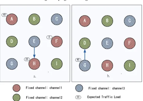
HMCMP would assign a long waiting time if there are many nodes sharing the same fixed channel. In Fig. 3a, node E wants to transmit packets with light traffic load to node H. In the case of light traffic load, it is not beneficial to set node E with a long waiting time even there are many nodes sharing the same fixed channel. On the other hand, in Fig. 3b, node G wants to transmit packets with high traffic load to node D. HMCMP
would assign a short waiting time because there is only one node D sharing channel 2 with node G. However, under a heavy traffic load, it is better to use a long waiting time to avoid collision. In this paper, we will consider a dynamic waiting time assignment algorithm based on both conditions of the traffic load and the number of nodes sharing the same channel.
2. Proposed Approach
In previous section, we show that it is not sufficient to assign the waiting time by just using the number of nodes sharing the same fixed channel. We will consider a waiting time assignment algorithm by taking the traffic load and the number of nodes sharing the same channel into account.
The probability of packet collision is proportional to the probability of packet transmission. Because collision only occurs in the receiver, we should keep
FST MaxSwitchTime of Ch2 WT2 DST2 SD FST MaxSwitchTime of Ch1 WT1 DST1
SD Data Transmit Time Data Transmit Time
SD : Switching Delay FST : Fixed Staying Time
WT1: Waiting Time for channel 1 DST1: Dynamic Staying Time for channel 1 WT2: Waiting Time for channel 2 DST2: Dynamic Staying Time for channel 2
Fig. 4 Staying Time Assignment
the record of the traffic load in the receiver. To estimate the traffic load for each receiving node, we propose to use the periodic broadcast “HELLO” message in every channel and let each node keep a data structure, called Channel Traffic Record List, CTRL, as shown in Fig. 5. In the periodic broadcasting message, the information of the CTRL list is included, which is an estimate of the traffic load for each channel. The traffic load for each channel is then proportional to the number of packets in the corresponding queue. From the receiving CTRL data, each node sums all of the traffic loads for each channel. It should be noted that although the proposed approach relies on the periodic broadcast “HELLO” message to collect neighbor information, it is not a heavy overhead.
Channel 1 2 3 4 … N
Load 2 40 50 0 … 3
Fig. 5 Example of CTRL
We summarize the proposed switching channel procedure in the following pseudo code:
Pseudo Code of Switching channel Procedure: Packet = Dequeue();
Channel = lookUpNeighobringTable( Packet ); if ( Channel == current channel ){
transmitPacket( Packet ); } else { CTRL = lookUpChannelTrafficRecordList(destination channel); T = caculateWaitingTime( CTRL ); switchChannel(destination channel); waitForWaitingTime( T ); transmitPacket( Packet ); }
where the function call lookUpChannelTrafficRecordList(destination channel)
will return an estimate of the traffic load from the neighbor nodes, whose information is contained in CTRL list, for the destination channel. The above pseudo code has clearly explained the channel switching procedure. In the following, we will explain how to calculate the waiting time, T, provided the traffic load is given.
In the switching channel procedure, nodes will calculate the waiting time for the new channel based on the Channel Traffic Record List (CTRL) and Channel Usage List (CUL). In general, the probability of collision is related to both conditions of the number of nodes sharing with the same fixed channel and the traffic load in the same channel. Either one of the
above two conditions just cannot do a good job in deciding the waiting time. Our point is that the waiting time should be decided by considering both conditions. We can divide the waiting time into two parts: the base waiting time and the dynamic waiting time. The base waiting time is the minimum period a node should wait after switching to a new channel. The dynamic waiting time is the interval of time a node after switching channel should wait until transmitting packets. We have gTime BaseWaitin tingTime DynamicWai e WaitingTim i= i+
where WaitingTimei denotes the waiting time for channel i. The dynamic waiting time, DynamicWaitingTimei,can be computed by:.
e WaitingTim ChannelMax X X tingTime DynamicWai i i= ×
where Xi denotes the total traffic load from the neighbor nodes sharing the same fixed channel, i, X is the maximum total traffic load. ChannelMaxWaitingTime is the maximal waiting time of this channel. The ChannelMaxWaitingTime is also dynamically assigned by considering the number of nodes sharing the same fixed channel.
Time MaxWaiting ber MaxNodeNum NodeNumber e WaitingTim ChannelMax = ×
where NodeNumber is the number of neighbor nodes sharing the same fixed channel, the MaxNodeNumber is the maximal number of the number of neighbor nodes to share the same channel, and MaxWaitingTime is the maximum waiting time. We note that the computation of the dynamic waiting time is based on both the number of neighbor nodes sharing the same channel and the estimate of the traffic load. The estimate traffic load is then determined by the queue length of the corresponding queue for the specific channel.
3. Simulation and Results
We used Qualnet 4.0 [20] to simulate the proposed protocols. In all simulations, nodes in the network were equipped with two IEEE 802.11b interfaces. The traffic is assumed to be constant bit rate (CBR), the basic rate is 1 Mbps, and the data rate is 11 Mbps. The duration of each simulation is 120 seconds. The transmission range of the nodes is set to be 250 m. The interface switching delay is assumed to be 1 ms. The packet size is fixed at 1024 Bytes. The number of channels is three as IEEE 802.11b provides. To
evaluate different waiting time settings, we compared the following three waiting time assignment schemes.
Fig. 6 (a) chain topology (b) grid topology
HMCMP-Static:
In this scheme, the waiting time is statically assigned to a period that is required to finish the transmission of a maximal sized packet. In all simulations, the waiting time is assumed to be 1899 ns. HMCMP-Dynamic
In this scheme, the waiting time is set as the original HMCMP scheme. That is, the waiting time is dynamically assigned according to the number of neighbor nodes sharing the same channel, as shown in Table 1.
Table 1 A set of the waiting time
number of fixed interfaces waiting time (us)
1 200 2 500 3 700 EHMCMP
In this scheme, the waiting time is determined by our proposed scheme that dynamically assigns the waiting time according to both conditions of the traffic loads and the numbers of nodes sharing the same channel. The MaxWaitingTime is assigned 1000 ns and BaseWaitingTime is assigned 100 ns. These two values are chosen by experimental observation. The maximum total traffic load X is determined according to the size of the network size.
We compared the above three schemes on two different topologies of nodes: the chain and the grid topologies, as shown in Fig. 6. We discuss the chain topology first. There are six nodes in a chain and nodes are away from their neighbors 200 m. The purpose of this experiment is to compare the aggregate throughput and the end-to-end delay in a multi-hop mesh network. There are two traffic flows in this topology: one of the
flows is from node 1 to node 6 and the other one is opposite. The fixed channel assignment adopts a uniform distribution. Thus the fixed channel of nodes is assigned as {ch1, ch2, ch3, ch1, ch2, ch3} for nodes from nodes 1 to 6. This kind of setting is managed to force nodes to switch their interfaces and increase the occurrences of the multi-channel hidden terminal problem.
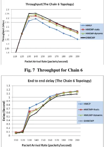
Fig. 7 Throughput for Chain 6
Fig. 8 End-to-end delay for Chain 6
Fig. 7 and Fig. 8 show the throughput and the end-to-end delay, respectively, in the topology of a chain with six nodes. Our proposed scheme EHMCMP has less end-to-end delay and more throughput than the static assignment HMCP, static, HMCMP-dynamic schemes.
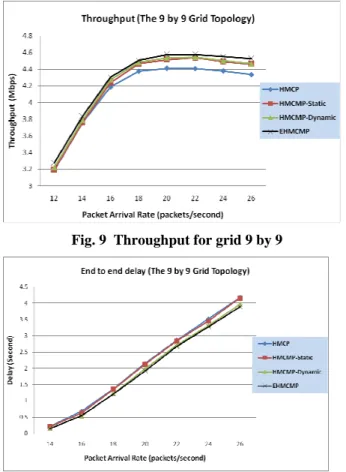
We then compared different waiting time assignment schemes in the grid topology with two kinds of traffic flows: static and dynamic traffic flows. We observed the results of the throughput and the end-to-end delay in multi-hop wireless networks with various sizes of grids: 3 by 3, 6 by 6 and 9 by 9. The distance between nodes was set to be 200 m. Since the obtained results are quite consistent in the various simulation settings, we will present the results for the 9 by 9 grids. The 9 by 9 grid is large enough to show the
Fixed channel: Ch1 Fixed channel: Ch2 Fixed channel: Ch3 (a)
advantages of dynamic waiting time assignment scheme. In all sizes of grids, our proposed scheme outperforms the other static or dynamic schemes in both the end-to-end delay and the throughput. When the traffic load is increasing, the improvements in the throughput and the end-to-end delay are more obviously observed.
In Fig. 9 and Fig. 10, we can see that the proposed EHMCMP scheme outperforms all the other schemes, including the HMCP, static, HMCMP-dynamic schemes. The improvement is more significant when the data rate increases. The throughput of the proposed scheme can improve up to 4.3% over the static scheme. The end-to-end delay can improve the static scheme up to 34.6% and as compared with the HMCMP-dynamic scheme, it also has up to 15.6% improvement. It is interesting to note that the improvement of end-to-end delay is more significant than that of throughput. This is because that reducing the waiting time has direct effects on the reduction of the end-to-end delay.
Fig. 9 Throughput for grid 9 by 9
Fig. 10 End-to-end delay for grid 9 by 9
4. Conclusion
In wireless mesh networks, the techniques of multi-channel multi-interface can utilize all channels effectively, providing more available bandwidth and more throughputs as well as reducing the end-to-end delay. In this paper, we have proposed an enhanced MAC protocol for multi-channel multi-interface wireless mesh networks. The proposed EHMCMP protocol makes use of both conditions of the traffic load and the number of nodes sharing the same fixed channel to dynamically assign the channel waiting time. Our point is that either condition alone cannot do a good job for deciding an appropriate waiting time. The simulation results show that our proposed scheme outperforms the other hybrid architecture protocols. We observed two metrics in the comparisons: one the throughput and another is the end-to-end delay. It is noted that the improvement of the end-to-end delay is more significant than that of the throughput. This is because that reducing the waiting time has direct effects on the reduction of the end-to-end delay. Another observation is that in terms of throughputs, as compared with the existing approach, the proposed scheme can only improve the throughput of 802.11b mesh networks up to 4.3%. This might be confined by the limited number of available channels, which are three non-overlapping channels provided by 802.11b networks in our Qualnet simulator. In future work, we may carry out more experiments for new techniques such as 802.11a or g.
5. References
[1] I.F. Akyildiz, X. Wang, W. Wang, Wireless mesh networks: a survey, Computer Network Journal (Elsevier), 47(4):445-487 2005
[2] P. Karn, “MACA- A New Channel Access Method for Packet Radio” Proc. ARRL/CRRL Amateur Radio Ninth Computer Networking Conference pp. 134-140 ARRL 1990
[3] IEEE, “IEEE Std 802.11-1999 Wireless LAN Medium Access Control (MAC) and Physical Layer (PHY) Specifications”, 1999
[4] S. Xu and T. Saadawi, “Does the IEEE 802.11 MAC protocol work well in multi-hop ad hoc networks?”, IEEE Community. Magazine., June 2001
[5] J. Jun and M.L. Sichitiu, The nominal capacity of wireless mesh networks, IEEE Wireless Communications Oct 2003 (5), pp. 8–14
[6] ”IEEE 802.11b Standard,”
standards.ieee.org/getieee802/download/802.11b-1999.pdf
[7] ”IEEE 802.11a Standard”;
standards.ieee.org/getieee802/download/802.11a-1999.pdf
[8] A. Raniwala and T. Chiueh, “Architecture and Algorithms for an IEEE 802.11-Based Multi- Channel Wireless Mesh Network,” in IEEE Infocom, 2005.
[9] S. Liese, D. Wu, P. Mohapatra “Experimental Characterization of an 802.11b Wireless Mesh Network ”ACM International Conference On Communications And Mobile,pp587-592 2006 [10] J. So and N. H. Vaidya, ”Multi-Channel MAC for
Ad Hoc Networks: Handling Multi-Channel Hidden Terminals Using A Single Transceiver,” ACM SIGMOBILE, pp. 222- 233, 2004.
[11] C.-Y. Chang, H.-C. Sun and C.-C. Hsieh, ”MCDA: An Efficient Multi-Channel MAC Protocol for 802.11 Wireless LAN with Directional Antenna,” In Proc. of AINA, vol. 2, pp. 64-67, 2005.
[12] A. Raniwal, K. Gopalan, T. Chiueh “Centralized channel assignment and routing algorithms for multi-channel wireless mesh networks”, - ACM SIGMOBILE Mobile Computing and Communications Review, vol. 8, no 2,pp55-65, April 2004
[13] P. Kyasanur and N.H. Vaidya, “Routing and Interface Assignment in Channel Multi-Interface Wireless Networks,” Proceedings of Wireless Communications and Networking Conference, 2005 IEEE. Vol. 4, pp. 2051 – 2056, Mar. 2005.
[14] P. Bahl, R. Chandra, J. Dunagan, “SSCH: Slotted Seeded Channel Hopping for Capacity Improvement in IEEE 802.11 Ad hoc Wireless Networks, in: ACM Annual International Conference on Mobile Computing and Networking (MOBICOM), 2004, pp. 216–230. [15] S.-L. Wu, C.-Y. Lin, Y.-C. Tseng and J.-P.
Sheu, ”A New Multi-Channel MAC Protocol with On-Demand Channel Assignment for Multi-Hop Mobile Ad Hoc Networks,” In Proc. of ISPAN, pp. 232-237, 2000.
[16] Y.-C. Tseng, S.-L., C.-Y. Lin and J.-P. Sheu, ”A Multi-Channel MAC Protocol with Power Control for Multi-Hop mobile Ad Hoc Networks,” In Proc. of CDCS, pp. 419-424, 2001. [17] C. -Y. Li, A. -K. Jeng, R. -H. Jan “A Medium
Access Control Protocol for Multi-Channel Multi-Interface Wireless Mesh Network”, Journal of Information Science and Engineering, Vol. 23, pp. 1041-1055, 2007.
[18] P. Kyasanur and N.H. Vaidya, ”Routing and Link-layer Protocols for Channel Multi-Interface Ad Hoc Wireless Networks,” ACM SIGMOBILE Mobile Computing and Communications Review, Vol. 10, No 1, pp. 31-43, 2006.
[19] J. Mo, H.-S. W. So and J. Walrand, ”Comparison of Multi-Channel MAC Protocols,” In Proc. of ACM SIGSIM, pp.209-218, 2005.
[20] Scalable Network Technologies, “Qualnet Simulator version 4.0” www.scalable-networks.com/