A HYBRID NEURAL NETWORK MODEL FOR SOLVING OPTIMIZATION PROBLEMS

218 IEEE TRANSACTIONS ON COMPUTERS, VOL. 42, NO. 2, FEBRUARY 1993

A Hybrid Neural Network Model

for Solving Optimization Problems

K.

T. Sun and H. C. Fu, Member, ZEEE

Abstract-In this paper, we propose a hybrid neural network model for solving optimization problems. We first derive an energy function, which contains the constraints and cost criteria of an optimization problem, and we then use the proposed neural network to find the global minimum (or maximum) of the energy function, which corresponds to a solution of the optimization problem. The proposed neural network contains two subnets: a Constraint network and a Goal network. The Constraint network models the constraints of an optimization problem and computes the gradient (updating) value of each neuron such that the energy function monotonically converges to satisfy all constraints of the problem. The Goal network points out the direction of convergence for finding an optimal value for the cost criteria. These two subnets ensure that our neural network finds feasible as well as optimal (or near-optimal) solutions. We use two well- known optimization problems-the Traveling Salesman Problem and the Hamiltonian Cycle Problem-to demonstrate our method. Our hybrid neural network successfully finds 100% of the feasible and near-optimal solutions for the Traveling Salesman Problem and also successfully discovers solutions to the Hamiltonian Cycle Problem with connection rates of 40% and 50%.

Index Terms-Energy functions, feasible solutions, neural net- work, optimization problems.

I. INTRODUCTION

EURAL networks have been used to solve a wide variety

N

of optimization problems [2], [lo], [14], [20], [22], [23], [28], [31]. Hopfield and Tank [8] suggested that the Traveling Salesman Problem [6] can be represented by an energy function that can be iteratively solved on a neural network. The difficulty in using a neural network to optimize an energy function is that the iteration procedure may often be trapped into a local minimum, which usually corresponds to an invalid solution. Moreover, the values assigned to the parameters of an energy function can greatly affect the convergence rate of iterations. Aiyer et al. [l] proposed a mathematical method for predicting a set of parameters on the Hopfield model that allow the Hopfield net to reach a feasible solution. However, Aiyer’s .method is still restricted to quadratic functions (the Hopfield net) only. Many optimization problems, such as satisfiability problems, cannot be solved by the Hopfield net. In this paper, we propose a hybrid neural network for solving energy functions of different orders. The solutions found by our network are all feasible.

Manuscript received February 15, 1991; revised September 10. 1991. This work was supported in part by the National Science Council under Grant The authors are with the Department of Computer Science and Information Engineering, National Chiao-Tung University Hsinchu, Taiwan 30050, R.O.C.

IEEE Log Number 9205428.

NSC 79-0408-E009-23.

We first express an optimization problem by a set of logical expressions and then map the logical expressions into algebraic equations. Based on these algebraic equations, an energy function is formulated. The energy function has two parts: constraints and the cost criteria. The proposed neural network also has two parts: a Constraint net (for the constraints) and

a Goal net (for the cost criteria). Benchmark tests on the

traveling salesman problem show that our neural network can provide 100% of the feasible and near-optimal (or optimal) solutions to the test problems.

The contents of this paper are as follows. In Section

11, we describe the proposed method for constructing an energy function from an optimization problem. In Section

111, we present the operations and functions of the proposed neural network model. A neural state updating method, the

coordinate Newton method, and some convergence theorems

are also introduced in Section 111. In Section IV, the results of experimental tests of our network are presented and discussed. Concluding remarks are given in Section V.

11. PROBLEM REPRESENTATION AND

THE TRANSFORMATION METHOD

Since Hopfield and Tank [SI constructed an energy function to represent the Traveling Salesman Problem (TSP) so that it could be iteratively solved on their neural network, many energy functions have been proposed to represent different optimization problems. To date, there is no systematic transfor- mation method for constructing an energy function to represent an optimization problem. In this section, we shall propose such a systematic transformation method. Our transformation method contains three steps: 1) representing an optimization problem as a set of logical expressions; 2) mapping these logical expressions into a set of algebraic equations; and 3) formulating an energy function from these algebraic equations. Each of these steps will be discussed as follows.

A. Representing an Optimization Problem by a Set of Logical Expressions

Since most optimization problems contain two parts: con- straints and cost criteria, to achieve an optimal solution, the constraints must he satisfied and the cost criteria must be minimized (or maximized). For example, in the Traveling Salesman Problem [9], the constraints are that each city must be visited exactly once and that a salesman can arrive at only one city at a time during the tour, and the minimization of the cost criteria is to find the shortest tour length. For this problem,

0018-9340/93$03 00 0 1993 IEEE

SUN AND FU: HYBRID NEURAL NETWORK MODEL FOR SOLVING OPTIMIZATION PROBLEMS 219 we use the logical symbol Czj or its complement to represent

whether or not a city z is being visited at time j during a tour, and we use the algebraic symbol d,, to represent the distance between cities z and y. Thus, the constraints and the minimization of cost criteria can be represented by the logical expressions at the bottom of this page and in the following.

In both of these constraints, N represents the number of

cities in the problem, and 1

5

i,j

5

N . Cost criteria: To find the shortest tour length.

where @ is an exclusive-OR operator (XOR).

Under constraints (1) and (2), the space of feasible solutions can be represented by a binary value matrix [ c ] N , N . In matrix [ C ] , there can be only one “1” (True) in each row and each column; all other variables must be “0” (False), so that constraints (1) and (2) are satisfied. Mapping logical expressions into algebraic equations is the second step of the transformation method. If we try to map expressions (1) and (2) directly into algebraic equations, however, the transformed algebraic equations will contain N N t h power terms, making it difficult and complicated to update the new value on a neural net and slowing down the convergence speed. Therefore, we propose to rewrite the constraints of the problem using shorter logical expressions with fewer state variables. The rewritten constraints and the logical expressions are as follows:

Constraint I : Each city i must be visited at least once and

no more than once. This constraint can be expressed by the

following set of logical equations:

\*

At least one Gib, 1

5

k

5

N , is True.

*\

\*

No more than one C i k , 1

5

k

5

N . is True.

*\

Constraint 2: A salesman arrives in at least one and no more than one city at any time j during the tour. Similarly, this

constraint can be expressed by the following set of logical equations:

\*

At least one C k j , 1

5

k

5

N , is True.

*\

Clj V Czj V C3j V . . . V CAT, = T r u e ,

\ *

No more than one C k j , 1

5

k

5

N , is True.

*\

Clj A C2j = False, Clj A C3j = False,

.

.

. ,

Clj A C N ~ = False,

Czj A Csj = False, . . .

,

C2j A C N ~ = F a l s e , . . .

,

CN-lj A Cp~j = False. ( 5 )

The logical expression “Cyi+l @ C,i-1 = True” in the cost

expression can also be formulated as

(Cyz+l A

c,i-1)

V

(Eyi+l

A

Cyi-l)

= False. ( 6 ) Now, we shall simplify the cost expression in (6) by eliminat- ing the term “(Cyi+l A C,i-l) = False, 1

5

y, i

5

N ” that

also appears in the constraints [Le., in (4)]. Thus, we can delete this term - from (6) so that expression - (6) can - be simplified to Cyz++l A C,i-1 = False. Since “Cyi+l A Cyi-l = False”

is logically equivalent to “C,i+l V C,i-1 = True,” the cost

expression then becomes

-

N N

M i n x x [ & , ( C , t A (c,i+l V C y i - l ) ) ] .

Now the constraints and the cost criteria of a TSP can be represented by expressions (4), ( 5 ) , and (7).

(7)

X,Y i

B. Mapping Logical Expressions into Algebraic Equations

By applying a mapping method similar to that used in

[29], logical expressions can be formulated as algebraic equa-

tions without changing their semantic meaning. The mapping method is listed as follows: Replace each instance of

1 ) True by 1 ,

2 ) False by 0,

3 ) Logical variable C%j by c ; j ,

4) A NOT operator by subtraction from one, and

5 ) An AND operator by multiplication.

Constraint 1: Each city i must be visited exactly once.

220 lEEE TRANSACTIONS ON COMPUTERS, VOL. 42, NO. 2, FEBRUARY 1993

When an OR operator is needed, it can be derived by com- bining the NOT and AND operators. For example,

xi

V =

Xi

A Y i . ( X i V

x)

can then be transformed into the algebraic equation 1 - (1 - x;)(1 - yi).

Based on this mapping method, the logical expressions of a TSP can be transformed into the following algebraic equations:

Constraint 1: Each city a must be visited at least once and no more than once.

-

C . Constructing an Energy Function from

the Algebraic Equations

function E, can be formulated as follows:

For the constraints of the TSP [(8) and (9)], a squared error

”

E , = C ( t i - (11)

i = l

where ti represents the target value (at the right-hand side) and

ai represents the iteration value (at the left-hand side) of each

algebraic expression of (8) and (9). N’ is the total number of algebraic equations in (8) and (9). An energy function E can be obtained by combining (10) and (11) as follows:

N’

E = E ,

+

C o s t = A c ( t i - ~ i

+

)BCost ~

where A and B are the parameters. When the constraints are satisfied (i.e., E, = 0) and the cost criteria is minimized, the shortest tour length of the TSP is obtained.

Parameter Setting: There are two adjustable parameters in

(12). Previous studies of neural networks for optimization problems have had to assign appropriate values to the param- eters in an energy function to find a feasible solution [l], [22]. Consequently, choosing improper values for the parameters in the energy function slows down the convergence speed and results in invalid solutions [l], [22]. In the next section, we propose a neural network and a neural state updating method in which the parameters of the energy function can be fixed values and no initial setting of the proper parameters is required. In addition, our method accelerates the convergence speed and generates feasible solutions.

(12) i=l 0 ... 1...0 Constraint Network

I

Network Goa’

1

1

Fig. 1. The structure of the hybrid neural network.

111. MINIMIZATION OF THE ENERGY FUNCTION Many neural network models and algorithms [4], [ll], [12], [MI-[20], [23], [30], [32] have been proposed for solving optimization problems. Most of the algorithms often converge to an invalid solution or require a large amount of computation time to reach an optimal (or near-optimal) solution. In this section, we propose a neural network model that finds an optimal (or near-optimal) solution within a short computation time.

The proposed neural network, which we called the hybrid neural network, contains two subnets: a Constraint network and a Goal network (see Fig. 1).

The Constraint network models the constraints of the prob- lem and computes the gradient (updating) value of each neuron (i.e., Ax1, Axz,

. . . ,

Ax,). By using these gradient value Ax’s, the Goal network computes the direction of convergence during each iteration for minimizing (or maximizing) the cost criteria (functions). The underlying point of this method is to ensure the constraints are satisfied (or at least are closer to being satisfied) at each stage of the gradient descent search on the cost functions. Therefore, the hybrid neural network produces feasible and near-optimal solutions.

We have designed an array processor system [5], [13] (see Fig. 2) for our hybrid neural network. In Fig. 2, each processor element (neuron) xi in the Constraint Net computes the updat- ing value Axi, and all updating values (Axl, Axz,

. . . ,

AZN)

are sent to the Max-Min Net to determine which neuron is to be updated. Each processor in the Goal net computes

F.

Both the Axi and are sent to the Max-Min net to determine which variable xi is to be updated. The output of the Max-Min Net enables the Selector module to output the corresponding updating value Axi, which will be passed

back to the input neurons to update their states. The iteration procedure continues until a stable state (i.e., Axi = 0) is reached.

The Coordinate Newton Method: To minimize the squared

error function E,, we propose a neural state updating method called the coordinate Newton method to compute the updating value of each neuron (i.e., each variable) at each iteration. This method is based on the concept of the coordinate descent method [17], in which a function f(z) is minimized with respect to one of the coordinate variables xi of z at each

SUN AND FU: HYBRID NEURAL NETWORK MODEL FOR SOLVING OPTIMIZATION PROBLEMS 221

Constraint Network

Goal Network

Fig. 2. The architecture of our hybrid neural network system.

iteration until the gradient of function f reaches zero (i.e., V f ( z ) = 0). In order to achieve faster convergence speed, we apply the Newton method [17] instead of the gradient method to search for the minimum. By using the Newton method to find the minimum of a function f , the updating value Ax for a vector

X

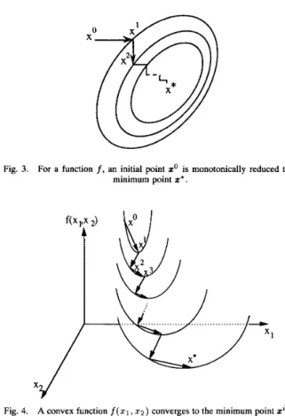
at an iteration t is defined by (13).

Fig. 3 .

Fig. 4.

For a function f, an initial point zo is monotonically reduced to a minimum point z * .

A convex function f(x1,xz) converges to the minimum point zi on the updating coordinate in each iteration.

AXt = [ F ( x ' ) ) l - l V f ( ~ X ~ ) ~ , and _{(potential) curve of a function f . The proof of this theorem}

is given in Appendix A.

Theorem 2: The coordinate Newton method always finds

(13)

- -

the minimum point of a function f along the updating coor- dinate at each iteration, where f has nonzero second-partial derivatives over a convex set

f2

in which each variable is of For updating a function

f

with only one variable x, (13) can

be simplified as

-

dx2

Thus, the updating value along a coordinate variable zi will be

where the value xi" is the new value on the coordinate xi such that the new point zt+l is closer to the minimum point. Some interesting properties of the coordinate Newton method are presented in the following theorems.

Theorem 1: The coordinate Newton method monotonically

reduces a function f to a stable state, where f has nonzero second-order partial derivatives over a convex set f2 in which each variable is of order two.

Fig. 3 illustrates that an initial point z'monotonically re- duces to a minimum point z* by the coordinate Newton method. Each ellipse curve in Fig. 3 represents an equal value

order two.

Theorem 2 means that the new point zt+l is the minimum point along the updating coordinate xi of the iteration t. The proof of this theorem is shown in Appendix B. Fig. 4 illustrates that an initial point z' of a convex function f ( x l r x 2 ) con- verges to the minimum point z1 along the updating coordinate 21. At the next iteration, the point 2' converges to the minimum point z2 along the updating coordinate 22, and the convergence procedure proceeds continuously until a stable point z* is reached (i.e., Of = 0).

Another property of the coordinate Newton method is that

it converges to a minimum with order two of convergence. Order of Convergence: When a sequence

{a}

converges to z*, the order of convergence [16] of {zk} is defined as the supremum of the nonnegative number p satisfying

(16)

-1

Xk+l - x*

I

O < lim

<

00.

k - i m

1

xk - x*

I p

A larger order of p implies a faster convergence speed.

Theorem 3: Let f be a function on

R".

Assume that there exists a minimum point z*, and the Hessian F ( z * ) is positive

222 IEEE TRANSACTIONS ON COMPUTERS, VOL. 42, NO. 2, FEBRUARY 1993 definite. If the initial point zo is not a minimum and it is

sufficiently close to z*, the sequence of points generated by the coordinate Newton method converge to

x*

with order two convergence.

The proof of this theorem is presented in Appendix C. From Theorem 3, the coordinate Newton method has the same convergence-of order two-as the Newton method. In order to apply the coordinate Newton method in the proposed neural network for solving optimization problems, we propose the following algorithm:

Hybrid Network Updating Algorithm (HNUA)

1.

2. 3.

4.

5 .

Apply the coordinate Newton method to minimize the squared error function E , by computing the updating

value Ax, (= &) for all variables (neurons) x,’s.

Calculate the partial derivative of the Cost function over

each variable xi (Le.,

F).

Determine the maximum value Ax* of N

I

A x , 1’s a E ,

a z 2

Ax* = Inax({[ Axi I,l

5

i

5

N } ) , ₍₁₇₎

then form a set

r

of variables x j that corresponds to the maximum updating value A x * , i.e.,

Among the x j variables in set I?, select a variable XI,

which corresponds to the minimum value of the partial derivative of the Cost function,

dCost

x,+ = min( - , v x j E

r).

a r g d x j

Update x i by adding the A x i obtained in Step 1,

=

+

ax;.

Check the gradient of function E , (i.e., V E , =

2,

Vi). If V E , is equal to OlxN, i.e., the energy function converges to a stable state (Axi = O,Vi), then stop. Otherwise, return to step 1 for the next iteration. The HNUA is implemented by the Constraint network and

the Goal network. Steps 1 and 2 can be executed in parallel on these two subnetworks. The max and min operations in steps 3

and 4 are performed by the Max-Min net. Based on the output from the Max-Min net, the Selector module selects the neuron

xk for updating. Finally, the Constraint net checks the gradient value V E , to see whether the iteration procedure should be

stopped or not. If the gradient V E , is equal to O l x ~ , then

the energy function has converged to a stable state, which represents a solution to the optimization problem.

We will apply the HNUA to solve two well-known opti- mization problems: the Traveling Salesman Problem and the Hamiltonian Cycle Problem.

Example 1: Traveling Salesman Problem (TSP): By apply-

ing the transformation method, the TSP can be represented by an energy function E [(12)]. The steps involved in using the

HNUA to solve the TSP are described as follows.

1. Apply the coordinate Newton method on the squared

error function E, [see ( l l ) ] to compute the Ac,, for

each variable czi, 1

5

x , i

5

N :

N dCost - _-

dzy(cyi+l+ cyi-i - c y i + i c y i - i ) . (23) acxi y=l,y#x

Determine the maximum value Ac* of N 2

I

Acxi )’s, Ac* = max({l Ac,, ) , 1

I

x , i

I

N } ) , (24) then form a set

r

of variables cyj that corresponds to the maximum updating value Ac*, Le.,

Among the cyj’s in set

r,

select a variable Cwk which

corresponds to the minimum value of the partial deriva- tive of the Cost function.

acost

,vcyj E

r).

c W k = min( -

arg dcyj

Update Cwk by adding the updating value obtained in Step 1.

Test the gradient of function E , (Le., V E , ) . If V E , is

equal to O1 N2, i.e., the energy function converges to a

stable state (i.e., Acxi = 0, Vx, i), then stop. Otherwise, return to step 1 for the next iteration.

Based on the HNUA, the squared error function E , of

the TSP monotonically converges to a stable state, because the squared error function E, has nonzero second partial

derivatives over a convex set in which each variable is of order two (see Theorems 1 and 2). Many interesting properties of the squared error function E, are presented with proofs in

Appendix D.

Example 2: Hamiltonian Cycle Problem (HCP): A Hamil-

tonian cycle in a graph G = (V, E ) is a cycle in graph

G containing all vertices in V. If G is directed, then the Hamiltonian cycle is directed; if G is undirected, then the Hamiltonian cycle is undirected. Note that not all graphs have a Hamiltonian cycle, and the problem of determining whether a graph G has a Hamiltonian cycle is NP-complete. To solve an HCP, we need to derive an energy function for the HCP. The energy function for an HCP can be derived in a way similar to the derivation of (12) for TSP. Since the nodes in an HCP are not fully connected, the cost (distance) d i j between nodes is defined as follows:

d i j = 1, if node i is connected to node j .

d i j = N , if there is no connection between node i and node j . (28) We represent the distance between two unconnected nodes i and j by a number N for ease of formulation and computation

SUN AND FU: HYBRID NEURAL NETWORK MODEL FOR SOLVING OPTIMIZATION PROBLEMS ₂₂₃

The procedure of using the Hybrid Network Updating Algorithm to solve an HCP is similar to the procedure for solving the TSP. To avoid repetition, in the following we will discuss only the major procedure differences between these two problems. For an HCP, a valid tour length is N for an N

nodes problem. The total distance connected to a node x at time i is equal to the value of

p.

Using the distance defined in (28), a value of greater than or equal to N indicates

a disconnected path to node x at time i . In order to continue searching for a connected cycle, we randomly select a node y

to visit at time i and remove the selected nodes at time i

+

1

and time i - 1. Thus, another path is tried in order to establish a complete cycle. This process can be seen as a hill-climbing technique used to escape from a spurious minimum z:and to search for the global minimum z* (an optimal solution).

From the TSP and HCP, we see that the coordinate Newton method is suitable for rapidly solving different optimization problems with different orders of the squared error function E,. Therefore, a wide variety of optimization problems, such as the satisfiability problem [23], the traffic control problem in interconnection networks [25], [26], the restrictive channel routing problem [27], the independent set problem, the multi- processor scheduling problem, and the partition problem can be also solved by this method.

IV. EXPERIMENTAL RESULTS

Simulation systems for the proposed neural network were constructed on an IBM RS/6000 workstation. The Traveling

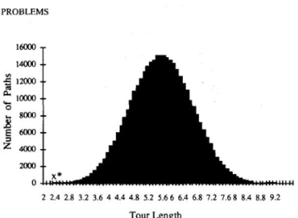
Salesman Problem (TSP) and the Hamiltonian Cycle Problem (HCP) were used as examples to test the performance of the proposed neural network. For the TSP, we tested 10, 50, 100 and 200-city problems with randomly chosen city coordinates within a unit square, similar to [21]. One hundred test cases with different city coordinates were simulated and tested for problems with different number of cities. The initial values of the neurons for different tests were all set to “O”, except for the starting city c11 (=1) of the tour. Fig. 5 shows the

tour length distribution for a 10-city TSP. For this case, our test result, 2.28, is an optimal solution. Table I shows our

simulation results along with the results for the Potts Neural Network ( N N , ) [21], Elastic Net (EN) [4], Genetic Algorithm (GA) [19], Simulated Annealing (SA) [ l l ] , Hybrid Approach (HA) [12], and Random Distribution (RD).

Using our neural network, the simulation time for solving a 200-city problem on an IBM RS/6000 workstation was

about two minutes. As shown in Table I, our results are

far better than those obtained by RD (random distribution), and our results are comparable to those for the Potts Neural Network (NN,). Although our method, HN, generates the longest or the second longest tour lengths, our object is to compare the overall performance of the different methods, including such factors as tour length, convergence speed, and feasible solution rate. As listed in Table I, our method is the only method that does not apply hill-climbing technique to escape from a local minimum. Obviously, applying hill- climbing technique requires a lot of computation. Davis [3] and Wilson et al. [30] have reported that some neural networks

2 2.4 2.8 3.2 3.6 4 4.4 4.8 5.2 5.6 6 6.4 6.8 7.2 7.6 8 8.4 8.8 9.2 Tour Length

Fig. 5. The distribution of tour lengths of a 10-city TSP. Our solution falls at the position z * (= 2.28), which is an optimal solution.

TABLE I

NETWORK (HN), Pons NEURAL NETWORK (NNp), ELASTIC NET (EN), GENETIC ALGORITHM (GA), SIMULATED ANNEALING (SA),

HYBRID APPROACH (HA), A N D RANDOM DISTRIBUTION (RD) COMPARISON OF AVERAGE TOUR LENGTHS DERIVED USING THE HYBRID

-v

Different Approaches (number ofcities) HN NNp EN GA SA HA RD 50 6.7 6.61 5.62 5.58 6.8 - 26.95 100 9.28 8.58 7.69 7.43 8.68 7.48 52.57 200 12.77 12.66 11.14 10.49 12.79 10.53 106.42

that do not use hill-climbing technique can become trapped into invalid solutions. Although our method guarantees that the solution search for the travelling salesman problem stops at the global minimum of the constraints, it may stop at the local minimum of the cost function. Thus we claim that our method generates feasible solutions for the TSP, although these solutions may not be optimal solutions. In addition, our method does not require setting proper values for the parameters in the energy function or estimating the temperature

T, for the annealing schedule, both of which are critical for

obtaining a good solution using the Potts Neural Network. The Elastic Net (EN) can only be applied to the TSP using geometrical distances between cities, which is too restrictive for the general TSP. The distances for a general TSP may contain costs, times, etc., and the Elastic Net cannot be used to solved this general problem. The genetic algorithm has the best performance, since it provides the shortest tour lengths. When a genetic algorithm is used, the solution is obtained after many evolutions of generations. In each generation, thousands of feasible solutions are generated, and the better solutions are selected to evolve the next generation. Therefore, using the genetic algorithm to compute a solution provides a higher probability of discovering a near-optimal solution than other methods, which generates only one result. However, the genetic algorithm requires a large amount of computation to find a solution. In addition, different operations of the genetic algorithm, such as crossover, mutation, and inversion, must be specially defined to solve different optimization problems. For example, the crossover operation in the genetic algorithm can be defined to exchange the positions of cities on the tour for the TSP, and it can also be defined to change the assignment of objects to different sets for partition problem.

224 IEEE TRANSACTIONS ON COMPUTERS, VOL. 42, NO. 2, FEBRUARY 1993 14000

-

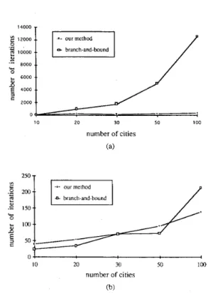
f, E 4000 .. a 10 20 30 50 100 number of cities (a) 250 T fn O J I 10 20 30 50 100 number of cities (b)

Fig. 6 . The number of iterations needed by our method and another efficient

algorithm to solve an HCP with connection density (a) 40% and (b) 50%.

So the genetic algorithm cannot provide a systematic method for solving different optimization problems. The simulated annealing (SA) method uses much time to reach a stable state, which makes it impractical for larger problems. The hybrid approach (HA), which combines three methods-the greedy method, simulated annealing, and exhaustive search-is a complex and computation-inefficient algorithm for solving the TSP. Compared with the other methods listed in Table I, our

method provides greater computational efficiency.

For the HCP, we also tested 10, 20, 30, 50, and 100-node problems with connection densities of 40% and 50%. One hundred tests with different connection distributions between nodes were simulated for each different size and density problem. A comparison of our method with the branch-and- bound algorithm [9], is shown in Figs. 6(a) and (b).

The branch-and-bound algorithm is a tree search procedure in which the number of iteration steps grows exponentially as the size of the problem is increased. However, our simulation results show that the number of iteration steps in our neural network approach grows approximately in linear. When the connection density is 50%, the results of our method are

comparable to those of the branch-and-bound algorithm. When the connection density is reduced to 40%, our method performs much better than the branch-and-bound algorithm. Our method seems to be suitable for solving HCP's with lower connection densities.

V. CONCLUSIONS

In this paper, a hybrid neural network and a neural state updating method for solving optimization problems have been proposed. A transformation method for representing an op-

timization problem by an energy function has also been presented. The transformation method can be applied to any type of optimization problem that can be represented by logical expressions such as those used in Section I1 of this paper. The energy function has two parts: the constraints and the cost criteria. It is solved using a hybrid neural network that comprises two subnets: the Constraint net and the Goal net, which correspond to the two parts of the energy function. The energy of the function is iteratively minimized (or maximized) by the neural network ~ operations until a

stable state is reached. The coordinate Newton method, a neural state updating method that combines the concepts of the coordinate descent method and the Newton method, is proposed for computing the updating value of each variable (neuron). Various merits of using the coordinate Newton

method to determine the gradient value of each variable in

order to reduce (or increase) the energy of the function are 1) the coordinate Newton method's convergence speed (order two convergence) is faster than that of the gradient descent method; 2) the coordinate Newton method is more suitable for parallel implementation than the Newton method; 3) if a function f has nonzero second-order partial derivatives over a convex set R in which each variable is of order two, then by applying the coordinate Newton method, a) the function f is monotonically reduced to a stable state, b) the function f always reaches the minimum point along the updating coordinate at each iteration; and 4) the stable state of the energy function represents a feasible solution.

In summary, the proposed neural network technique for solving optimization problems has the following advantages:

1) It provides a mapping technique for systematically trans- forming an optimization problem into an energy func- tion.

2) It does not require selection of the proper values for parameters in an energy function in order to obtain an optimal (or near-optimal) solution.

3) It prevents the energy function from being trapped into an invalid solution.

APPENDIX A PROOF OF THEOREM 1

The coordinate Newton method monotonically reduces a function f to a stable state, where f has nonzero second- order partial derivatives over a convex set R, in which each variable is of order two.

Proof: According to Taylor's series expansion, we can

expand a function f ( z ) at point z0 as follows:

1 1

f ( z ) = f ( ~ ~ ) + d f ( ~ ~ ) + - d ~ f ( z O ) i 3 d ~ f ( ~ ~ ) + . . . 2!

,

(29)

f Po ) where d k f ( z O ) =

E,1

cz2

.

. .

Czk

a z l B x z azn qiqz

. .

and qz = x, - 2 : . By applying the coordinate Newton method,

the updating value of 2 , along the coordinate 2 , at iteration t is

afo

ax: 2t+l - 2 ; - aZ, z a z f ( x ' )

'

and 2;" = xi, VJ

#

r . - (30)

SUN AND FU: HYBRID NEURAL NETWORK MODEL FOR SOLVING OPTIMIZATION PROBLEMS

~

225 kt z 1 xt+' and zo = xt. Then q; = x i -

~4

= - x: =

Ax;, such that the value of qi is equal to Axi. Rewrite (29) in terms of z t , x t t l and A z . Then

1 d3f(zt)

3! dX?

+

-Ax: ~

+

.

.

.

.

Since each variable in function f is of order two, the higher order terms (&Ax?-

+

. .

.) vanish and (31)'becomes

axt

Then,

1 (*)2

A f ( z t ) = 2 a 2 f ( z t ) ' (33)

ax:

Since f ( z ) is a convex function, the second partial derivatives of function f ( z ) are greater than 0 (i.e.,

>

0). Therefore, we can prove that

A f ( z t )

5

0. (34)

This implies that the' function

f

is monotonically reduced to

a stable state. Q.E.D.

APPENDIX B PROOF OF THEOREM 2

The coordinate Newton method can always find the mini- mum point of a function f along the updating coordinate at each iteration, where f has nonzero second-partial derivatives over a convex set R in which each variable is of order two.

Proof: The function f ( z ) , z = (xl, 2 2 , .

. . ,

zn), can be expressed in terms of the variable X, as follows:

f ( z ) = Ex:

+

Fx,

+

G , and E

>

0; F, G E R, ₍₃₅₎ where E , F and G are the terms that contain variables x l , V j

#

i in the function f ( z ) . By applying the coordinate Newton method to function f on the coordinate 2 % ) the variable

x,

is

updated by

afo

-az,

₍₃₆₎

W '

If new point z' is the minimum point on the coordinate z,,

then the partial derivative of f over X, at the next iteration should equal zero.

d

+

--xi

a

+

0

dxa d X 2

= 2 E ( 1 - l)

+

F ( l

-

l )

= o + o

= 0 . (37)

From the minimization of convex functions, (37) shows that the new point z' is the minimum point on the coordinate x i at the next iteration. Thus, the coordinate Newton method always finds the minimum point along the updating coordinate at each

iteration. Q.E.D.

APPENDIX C PROOF OF THEOREM 3

Let f be a function on R". Assume that there exists a minimum point z* and that the Hessian F ( x * ) is positive

definite. If the initial point zo is not a minimum and is sufficiently close to z*, the sequence of points generated by the coordinate Newton method converge to

x*

with order two convergence.

Proof: According to the coordinate Newton method, the

updating value for each neuron is x:+' = xr + A x : , which can

be represented in vector form for the purpose of proving the convergence of the function f . In vector form the updating value is

%t+l = zt - [ e , F ( z t ) e r ] - ' V f ( z t ) e r e , (38) where e, is the zth coordinate unit vector (i.e., el =

(1,O,O

, . . . ,

O),e2 = (O,1,O

,...,

0) , . . . , e , = (O,O,O

,...,

1)); F ( x t ) is the Hessian matrix [17], [ d 2 f / d x , d x , ] , V z , ~ ,

of the function f ; and V f ( z t ) is the gradient of function f at time t . There exists p, a

>

0,

p

>

0 such that

1

z

-

x*

I<

p,

I

[e,F(x)e:]-'

I

5

a and

I

V f ( z ) e F e ,

+

[e%F(x)eT](z* - z)

15

p

I

z - z*

12,

for all z. Now suppose zt is selected

with a.P

I

zt - z*

I<

1. Then

I

zt+' - z*

I =I

zt - z* - [ e Z ~ ( x t ) e T ] - ' o f ( z ' ) e F e ,

I

=I

[ e Z ~ ( z t ) e r ] - ' ( ~ f ( z t ) e ~ e ,

+

[ e Z ~ ( z t ) e r ] ( z *

-

z'))

I

51 [ e , ~ ( z ~ ) e ? l - + l

1 0

1

zt - z*

l2

-

<

ap

I

xt - z* 12 ₍₃₉₎ < ) z t - z *

I .

(40)

Equation (40) shows that the new point zt+' is closer to z* than the point zt, and (39) shows that the order of convergence of the coordinate Newton method is two. Q.E.D.

APPENDIX D PROPERTIES OF THE SQUARED

ERROR FUNCTION E, OF THE TSP

Property 1: Based on the coordinate Newton method, the value of each variable cxi, 1

5 x,

i

5

N , in the squared error function E, is bound within [0,1].

226 IEEE TRANSACTIONS ON COMPUTERS, VOL. 42, NO. 2, FEBRUARY 1993

Proof: The squared error function E, [(ll)] can be

rewritten as

E, =

7;

yI

+

c$icii

z i j # i x y f z i

x i i x

Equation (41) can be expressed in terms of the variable cxi:

E, = A&

+

Bcxi

+

C , (42)

where A 2 0, C 2 0, and B

5

0. Therefore, (42) is a convex function of cxi and can be expressed as

B B2 B2 E, = A ( c ; ~

+

-c,i

+

-)

+

C - - A 4A2 4 A (43) B B2 = A ( c X i

+

- ) 2

+

C -

-.

2 A 4A (44)

From Theorem 2, is equal to the minimum point (=

g )

at iteration

t

+

1 , so the value of the variable c,i is bound by

(45) From (41), the value of A (summation of the terms with order two) is greater than or equal to f B (summation of the terms with order one), thus c::’ is further bound by

(46)

t+l - -B

cxi - ~

<

1.

2 A -

This proves that the value of the variable e,; is bound by

[OJ]. Q.E.D.

Property 2: For the neuron state matrix [ C ] N x N of a TSP, when the value of a variable e,; equals one and the values of

other elements in row z and column i are not all zeros, then the gradient value of

2

is not equal to zero.

Proof: When more than one variable in a row z and column i is one and the values of the other elements in row

z and column i are not all equal to zero, (45) shows that the gradient value of

E

is not equal to zero (not in a stable

state). Q.E.D.

Property3: By applying the HNUA, when the squared

error function E, reaches a stable state and a variable c,i equals one, then each row and each column of matrix [ q n r X N must contain only one “1” and all other entries of this row and column must be “0”, which corresponds to a feasible solution.

Proof: From (41), the first-order partial derivative of E,

with respective to the variable e,, is

When the function E, reaches a stable state and the value of e,, is equal to one, (47) becomes

aEs dcx,

-

= 2[c;1

+

c22

+

’ ’ ’

+

cE,-l

+

c:,+1

+

. . .

+

+

e:,

+

e;,

+

. ’ .

+

c;-1,

+

+

. . .

+

e”,]

= 0 , 1 < z , i

5

N . ₍₄₈₎

Since (48) contains only squared terms, all variables in row z

other than c,, must be zero. Similarly, on the stable state, the partial derivative 2 , V l

#

i , must be zero. Then,

aE, dcxl

-

= -2(1 - c11)2(1 - c21)2..

.

(1 - C X - 1 l ) ( l - cx+11)2 . ’ ‘ ( 1 - C N [ ) 2 = 0, Vl

#

a. (49)

From property 2, there exists only one element cpl that is “1” in column 1 of matrix [ C ] N , N , and the other elements are all zeros. Similarly, we can prove that any row or any column

contains only one “1.” Q.E.D.

ACKNOWLEDGMENT

We are grateful to Profs. S. Y. Kung and J. N. Hwang and C .

C . Chiang for their helpful discussions and suggestions. Also,

we wish to thank anonymous reviewers for their insightful comments.

REFERENCES

S. V. B. Aiyer et al., “A theoretical investigation into the performance of the Hopfield model,” IEEE Trans. NeuralNetworks, vol. 1, pp. 204-215, June 1990.

B. Angeniol, G. De La Croix Vaubois, and J.-Y. Le Texier, “Self- organizing feature maps and the travelling salesman problem,” Neural Networks, vol. I, pp. 289-293, 1988.

G. W. Davis, “Sensitivity analysis in neural net solutions,” IEEE Trans. Syst., Man, Cybern., vol. 19, no. 5, pp. 1078-1082, 1989.

R. Durbin, R. Szeliski, and A. Yuille, “An analysis of the elastic net approach to the traveling salesman problem,” Neural Computat., vol. 1, p. 384, 1989.

H. C. Fu, J. N. Hwang, S. Y. Kung, W. D. Mao, and J. A. Vlontzos, “A universal digital VLSI design for neural networks,” in Proc. IJCNN’89,

Washington DC, June, 1989.

M. R. Garey and D. S. Johnson, Computers and Intractability: A Guide

io the Theory of NP-compleness. San Francisco, CA: Freeman, 1979.

K. M. Gutzmann, “Combinatorial optimization using a continuous state Boltzmann machine,” in Proc. IEEE First Int. Conf Neural Networks,

vol. 111, San Diego, CA, June 1987, pp. 721-728.

J. J. Hopfield and D. W. Tank, “Neural composition of decisions optimization problems,” vol. 55, pp. 141 - 152, 1985.

E. Horowitz and S . Sahni, “Dynamic programming,” in Fundamentals of Computer Algorithms. Rockville, MD: Computer Science Press, 1978.

J. J. Johnson, “A neural network approach to the 3-satisfiability prob- lem,” J . Parallel Distributed Comput., pp. 435 -449, 1989.

S. Kirkpatrick, C. D. Gelatt, and M. P. Vecchi, “Optimization by simulated annealing,” Science, vol. 220, p. 671, 1983.

S. Kirkpatrick and G. Toulouse, “Configuration space analysis of the traveling salesman problem,” J. Phys., vol. 42, p. 1277, 1985.

S. Y. Kung, VLSI Array Processors. Englewood Cliffs, NJ: Prentice- Hall, 1988.

B. W. Lee and B. J. Sheu, “Combinatorial optimization using competitive-Hopfield neural network,” in Proc. Int. Joint Conf Neural Networks, vol. 11, Washington DC, Jan. 1990. pp. 627-630, R. P. Lippmann, “Introduction to computing with neural nets,” IEEE

ASSP Mag., pp. 4-22, Apr, 1987.

D. G. Luenberger, “Speed of convergence,” in Linear and Nonlin-

ear Programming. Reading, MA: Addison-Wesley., 1984, ch. 6, pp. 189-192.

SUN AND FU: HYBRID NEURAL NETWORK MODEL FOR SOLVING OPTIMIZATION PROBLEMS 227 -, “Basic descent methods,” in Linear and Nonlinear Program-

ming.

S. Mehta and L. Fulop, “A neural algorithm to solve the Hamiltonian cycle problem,” in Proc. Int. Joint Conf Neural Networks, vol. 111, San

Diego, CA, June 18-22, 1990 pp. 843-849.

H. Muhlenbein, M. Gorges-Schleuter, and 0. Kramer, “Evolution al- gorithms in combinatorial optimization, Parallel Computat., vol. 7, p.

65, 1988.

C. Peterson and B. Soderberg, “A new method for mapping optimization problems onto neural networks,” Int. J. Neural Syst., vol. I, pp. 3-22,

1989.

C. Peterson, “Parallel distributed approaches to combinatorial optimiza- tion: Benchmark studies on the traveling salesman problem,” Neural Computat., M.I.T. Press Journals, vol. 2, pp. 261-269, 1990.

J. Ramanujam and P. Sadydppan, “Parameter identification for con-

strained optimization using neural networks,” in Proc. 1988 Connec- tionist Models Summer School, Morgan Kaufmann, 1988 pp. 154- 161.

K. T. Sun and H. C. Fu, “Solving satisfiability problems with neural networks,’‘ in Proc. IEEE Region I O Con5 Comput. and Commun. Syst.,

vol. 1, Hong Kong, Sept. 24-27, 1990, pp. 17-22.

-, “A neural network for solving the satisfiability problems,” in

Proc. Int. Comput. Symp. 1990, National Tsing Hua University, Taiwan,

R.O.C., Dec. 17-19, 1990 pp. 757-762.

-, “An O(n) parallel algorithm for solving the traffic control problem on crossbar switch networks,” Parallel Processing Lett. (PPL),

vol. 1, no. I, pp. 51-58, 1991.

-, “A neural network algorithm for solving the traffic control problem in multistage interconnection networks,” in Proc. Int. Joint Con$ Neural Networks (IJCNN-91), Singapore, Nov. 24-28, 1991 pp.

1136- 1141.

-, “A neural network approach to restrictive channel routing problems,” in Proc. Int. Conf: Artificial Networks ICA”’92. G . A. Taglianeri and E. W. Page, “Solving constraint satisfaction

problems with neural networks,” in Proc. Int. Conf Neural Networks,

San Diego, CA, June 1987, pp. 741-747.

R. J. Williams, “Learning the logic of activation functions,” in Parallel Distributed Processing, Vol. 1. Cambrideg, M A M.I.T. Press, 1986,

ch. 10, pp. 423-443.

G. V. Wilson and G. S. Pawley, “On the stability of the travelling salesman algorithm of Hopfield and Tank,” Biol. Cybern., vol. 58, pp.

63-70, 1988.

X. Xu and W. T. Tsai, “An adaptive neural algorithm for traveling salesman problem,” in Proc. Int. Joint Conf: Neural Networks, vol. I,

Washington, DC, Jan. 1990, pp. 716-719.

Reading, MA: Addison-Wesley, 1984, ch. 7, pp. 197-237.

[32] A. Yuille, “Generalized deformable models, statistical physics, and

matching problems,” Neural Computat., vol. 2, pp. 1-24, 1990.

K. T. Sun received the B.S. degree in information science from Tunghai University in 1985 and the

M.S. and Ph.D. degrees in computer science and

information engineering from National Chiao-Tung University in 1987 and 1992, respectively.

He is a Research Associate in Chung Shan In- stitute of Science and Technology, and an Adjunt Associate Professor at the Information Science De- partment in Tunghai University, Taiwan, R.O.C. His research interests include logical programming, par- allel processing, array processors, fuzzy theorems, and neural networks.

H. C. Fu (S’79-M’80) received the B.S. degree

in electrical and communication engineering from National Chiao-Tung University in 1972, and the

M.S. and Ph.D. degrees in electrical and computer

engineering from New Mexico State University in

1975 and 1981, respectively.

From 1981 to 1983 he was a member of Technical Staff in Bell Laboratories. Since 1983 he has been on the faculty of the Department of Computer Sci- ence and Information Engineering, National Chiao- Tune Universitv. Hsinchu. Taiwan. R.O.C. From Y ,,

1987 to 1988, he was a Director of the Department of Information Manage-

ment at the Research, Development and Evaluation Commission in Executive Yuan, R.O.C. In the academic year 1988-1989, he was a Visiting Scholar at Princeton University. From 1989 to 1991, he was the Chairman of the Department of Computer Science and information Engineering at N.C.T.U., where he is currently a Professor there. He is the author of over 40 technical papers in computer engineering. His current research interests are in computer architecture, array processing, parallel processing, and neural computing.

Dr. Fu is a member of the IEEE Computer Society, Phi Tau Phi, and the Eta Kappa Nu Electrical Engineering Honor Society.