A fast convolution algorithm for biorthogonal wavelet image compression

This article was downloaded by: [National Chiao Tung University 國立交通大學] On: 28 April 2014, At: 03:45

Publisher: Taylor & Francis

Informa Ltd Registered in England and Wales Registered Number: 1072954 Registered office: Mortimer House, 37-41 Mortimer Street, London W1T 3JH, UK

Journal of the Chinese Institute of Engineers

Publication details, including instructions for authors and subscription information: http://www.tandfonline.com/loi/tcie20

A fast convolution algorithm for biorthogonal wavelet image compression

Bing‐Fei Wu a _{& Chorng‐Yann Su} b a

Department of Electrical and Control Engineering , National Chiao Tung University , Hsinchu, Taiwan 300, R.O.C.

b

Department of Industrial Education , National Taiwan Normal University , Taipei, Taiwan 106, R.O.C. Published online: 02 Mar 2011.

To cite this article: Bing‐Fei Wu & Chorng‐Yann Su (1999) A fast convolution algorithm for biorthogonal wavelet image compression, Journal of the Chinese

Institute of Engineers, 22:2, 179-192, DOI: 10.1080/02533839.1999.9670455

To link to this article: http://dx.doi.org/10.1080/02533839.1999.9670455

PLEASE SCROLL DOWN FOR ARTICLE

Taylor & Francis makes every effort to ensure the accuracy of all the information (the “Content”) contained in the publications on our platform. However, Taylor & Francis, our agents, and our licensors make no representations or warranties whatsoever as to the accuracy, completeness, or suitability for any purpose of the Content. Any opinions and views expressed in this publication are the opinions and views of the authors, and are not the views of or endorsed by Taylor & Francis. The accuracy of the Content should not be relied upon and should be independently verified with primary sources of information. Taylor and Francis shall not be liable for any losses, actions, claims, proceedings, demands, costs, expenses, damages, and other liabilities whatsoever or howsoever caused arising directly or indirectly in connection with, in relation to or arising out of the use of the Content.

This article may be used for research, teaching, and private study purposes. Any substantial or systematic reproduction, redistribution, reselling, loan, sub-licensing, systematic supply, or distribution in any form to anyone is expressly forbidden. Terms & Conditions of access and use can be found at http://www.tandfonline.com/page/terms-and-conditions

Journal of the Chinese Institute of Engineers, Vol. 22, No. 2, pp. 179-192 (1999)

A FAST CONVOLUTION ALGORITHM FOR BIORTHOGONAL

WAVELET IMAGE COMPRESSION

Bing-Fei Wu*

Department of Electrical and Control Engineering National Chiao Tung University

Hsinchu, Taiwan 300, R.O.C. Chorng-Yann Su

Department of Industrial Education National Taiwan Normal University

Taipei, Taiwan 106, R.O.C.

Key Words: fast convolution algorithm, wavelet image compression, symmetric extension, zerotree coding.

ABSTRACT

Symmetric filters and symmetric extension of image edges have been widely used in wavelet image compression. Since the filters are symmetric, it is possible to take advantage of the symmetric property to reduce the computational complexity for the filtering. In this paper, we present a fast convolution algorithm for the discrete wavelet trans-form (DWT) and the inverse DWT (IDWT) such that the transtrans-form time can be greatly reduced. Compared with regular convolution, the new algorithm can decrease the multiplication operations by nearly one half. Converted into real programming, it sped up the DWT and IDWT in our experiments by at least 12% and 55%, respectively. Incorpo-rated with enhancing zerotree coding, the proposed algorithm results in a rapid and efficient coder. Experimental results showed that the coder is competitive with other high performance coders. The pro-posed convolution algorithm is also suitable for many types of wave-let-based coding, including wavelet video coding.

I. INTRODUCTION

Transform coding is a favorite technique in im-age compression. It has become a key component in international video communication standards (Pennebaker and Mitohell, 1993). In the past de.cade, the discrete cosine transform (DCT) has bee.n tfygmost popular transform because it provides almost optimal performance and can be implemented at an accept-able cost. However, recently the discrete wavelet transform (DWT) has received more attention because

it can solve the blocking effect introduced by the DCT and it is particularly well adapted to progressive trans-mission (Antonini et al., 1992). Furthermore, the pyramid-like multiresolution decomposition by the DWT can produce some degree of self-similarity across different scales, which is helpful in image com-pression.

Shapiro (1993) has introduced the embedded zerotree wavelet (EZW) algorithm, (Shapiro, 1993) which takes advantage of the features of DWT, and he has shown that the EZW is not only competitive

†Invited paper

*Correspondence addressee

180 Journal of the Chinese Institute of Engineers, Vol. 22, No. 2 (1999)

in its performance with the most complex techniques, it is also extremely fast in its execution. In addition, the set partitioning in hierarchical trees (SPIHT) (Said and Pearlman, 1996) and the space-frequency quan-tization (SFQ) algorithms (Xiong et al., 1997), etc., have also shown that DWT-based coders obtain per-formances much superior to JPEG or to most of the other DCT-based coders. Specifically, SPIHT inter-rupts the simultaneous progression of efficiency and complexity. It is almost the best coder in the litera-ture no matter if the comparison concerns perfor-mance or execution time. Because of the advantages of DWT-based coders, Martucci et. al. (1997), have transferred DWT-based techniques from gray level image coding to video compression.

However, many of the high performance DWT-based coders, such as EZW and SPIHT, have to take most of the CPU time to perform the transformation. Thus, reducing the transform time in DWT or inverse DWT (IDWT) is the crucial issue in decreasing the total execution time of these coders. This problem has motivated researchers to develop fast convolu-tion algorithms for DWT IDWT.

Two approaches are frequently used to improve performance in wavelet image compression. One approach selects a pair of biorthogonal linear phase filters, and the other approach uses symmetric exten-sion of the image edges (Said and Pearlman, 1996; Xiong et al., 1997). It is well-known that orthogonal wavelets have the merit of energy preservation. How-ever, the orthogonal wavelets are highly constrained, which allows for little design flexibility. For ex-ample, it is desirable that the finite impulse response (FIR) filters used are of the linear phase, since such filters can be easily cascaded in the pyramidal filter structures without phase compensation (Antonini et al., 1992) and the corresponding coder can obtain improved performance. Unfortunately, there are no orthogonal linear phase FIR filters with the exact re-construction property except for some trivial cases (such as the Haar filter). To preserve the linear phase (corresponding to the symmetry for the wavelet) prop-erty, one can relax the orthogonality requirement by using biorthogonal bases. In this case, biorthogonal wavelets are not used for energy preservation. Some biorthogonal filters (such as 9/7-tap (Antonini et al., 1992)) are designed to be "close" to orthogonal, so that the quantizers designed in the orthogonal case can be well approximated. In a two-channel filter bank, there are three forms of biorthogonal linear phase filters that can achieve perfect reconstruction (Vetterli et al., 1995). In the most popular form both filters are symmetric and are of odd lengths in the analysis bank. Since the filters are symmetric, sym-metric extension of the image edges can be applied. The advantage of using symmetric extension is that

the number of jumps between the transformed coef-ficients can be reduced. These jumps are probably introduced by the circular extension of the image edges because the gray levels between the first pixel and the last are generally different in the same row or column.

Martucci (1994) used the so-called symmetric convolution to convolve symmetrically extended se-quences. To use symmetric convolution to filter a sequence, one should first retrieve the right-half samples of a symmetric filter. Next, apply the ap-propriate symmetric extensions to the retrieved se-quence and to the input sese-quence, and then obtain the convolution results with the following two methods. One method involves the application of a circular or skew-circular convolution to both of the symmetri-cally extended sequences, and then a rectangular win-dow is used to extract their representative samples out of the base period. The other method involves taking an inverse discrete trigonometric transform (DTT) from the product of the forward DTTs of these two sequences. In this paper, we will develop a fast convolution algorithm that is similar to the former method, but our algorithm is a much more straight-forward approach. The proposed algorithm is mainly applied while the symmetric filter is of odd length and the image edges are symmetrically extended. Because both the filter and the image extension are symmetric, many terms of the multiplied results will be computed repeatedly while filtering an image. Hence, if we can efficiently permute the nonrepeated terms and sum up some of the terms for each differ-ent transformed coefficidiffer-ent, then we can reduce the multiplication operations by nearly one half. This is the main idea proposed in this paper. The most at-tractive feature of our new algorithm is the simplic-ity of its final form. This approach provides easy implementation without additional computational complexity.

In the following sections, we will address the algorithm for the one dimensional (1-D) case, whose results can be extended to filter higher dimensional sequences by using the 1-D case for each dimension, independently. Section II describes the regular con-volution in 1-D DWT and IDWT, which is often used in real programming. Section III and Section IV il-lustrate the frameworks of the proposed fast convo-lution algorithms for DWT and IDWT, respectively. The analysis concerning the computational complex-ity is shown in Section V. Experimental results, including the execution time, are shown in Section VI. To contrast the performance of different exten-sions of the image edges, we incorporate the proposed algorithm into our previous coder based on an enhanc-ing zerotree codenhanc-ing (Wu and Su, 1998). Some recon-structed images at a bit rate 0.5 bits per pixel (bpp)

and the results of the peak signal to noise ratios (PSNR) at various bit rates are illustrated in this sec-tion. The conclusion of this paper is given in Section VII.

II. The 1-D DWT AND IDWT

The two-channel 1-D DWT of a sequence a[n] (see Fig. 1) is defined as

= T,h[2k-n]a[n] n

Analysis Synthesis

where A[k] and B[k] represent the sequences produced from the lowpass and the highpass channels, respec-tively. Eq. (1) describes a convolution scheme fol-lowed by a downsampler with sampling period being 2. With biortho-gonal wavelets, the corresponding IDWT to reconstruct a[n] is given as

a[n]=ao[n]+ax[n]

(2)

where ao[n] anc* ai M indicate that the reconstructed

sequences are contributed to by the lowpass and highpass channels, respectively. In order to have a perfect reconstruction, we set

\yh[l-n], g[n]=(-T,h[n]h[n+2m] =

-n], and

(3)

So far, there is nothing different from usual subband coding schemes. To distinguish the wavelet decomposition from the usual subband coding schemes, the following constraints in the filters are also imposed (Anotnini et al., 1992)

= 0 and £ ( - l)"h[n] = 0 . (4)

In the above equations, all of the filters and the sequence are infinite. However, the finiteness on fil-ters and the sequence have to be considered in the real application. The immediate problem of Eq. (1) is how to compute the product h[2k-n]a[n] if the in-dex in the bracket is out of the defined range. For example, the filter h[n] is assumed to be with only positive index terms defined at 0, ..., L - l , and the computation in Eq. (1) may ask for h[-l] which is not defined. One possible solution for solving this fi-nite length issue is to perform the N-point circular

Convolve with filter X

,2 I Downsamplingby 2

Upsampling by 2

Fig. 1. Two-channel filter bank and the associated wavelets.

convolution (Oppenheim and Schafer, 1989) (assume that the sequence length is N and N>L). To do this, the filter h[n) has to be zero-padded. Since the prod-uct of a value multiplied with a zero does not con-tribute anything to the convolution sum, the compu-tation is tedious and a waste of time. A better method is to sum up only the possible nonzero terms. This can be done by computing Eq. (1) based on the filter length. Therefore, we rewrite Eq. Eq. (1) to

= Zh[n]a[2k-n],

(5) This is feasible in the linear and time invariant (LTI) systems. Consequently, the number of multiplication operations (NMOs) in Eq. (5) is L for each A[k] or B[k]. It is, generally, far fewer than those required in Eq. (1) (the required NMOs is N for each A[k] or B[k]). For the same reason, Eq. (2) is rewritten as

a[n] = £ h[k]A[(k + n)l2\ + Z g[k]B[(k + n)l2],

k k

for k+n=2l, leZ. (6)

We refer to this type of convolution based on the fil-ter length as the regular convolution, which is com-monly used in real programming.

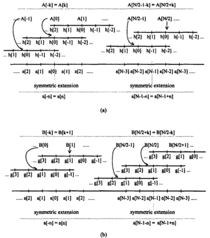
In Eq. (5), the same problem is how to compute the products when the index of a[n] is out of the de-fined interval. There are two possible solutions to solve this. One solution is to extend the sequence a[n] by circular extension (Fig. 2(a)), and the other is to extend it by symmetric extension (Fig. 2(b)). Circular extension and symmetric extension for the image edges are shown in Fig. 2(c) and Fig. 2(d), re-spectively. Circular extension is the most widely used solution in digital signal processing. This extension is suitable for all filters, but introducing possible jumps at the endpoints is its disadvantage because generally a[N-l] does not equal a[0]. The jumps introduced into the process will lower the coding performance when using the EZW-like algorithms.

Journal of the Chinese Institute of Engineers. Vol. 22. No. 2 (1999)

.|-nl=.|Vn|

- 1 0 1 2 . . NO N-l N Hi

(a) Circular cxlcmim

•J-")-.)"! ^N.|*n|-«[N-l-n|

I 1 1 1 1 1 1

N-2 N - l N N - l N+2 ..

n Symmcirt cxwn

(•ii! 1 Circular extension and symmetric extension (s) eircttlai extension in a sequence ihi symmetric extension in n se-quence H I circular extension oJ Image edgesfd] tymmei iii extension oi Image edges

As For symmetric extension, ii is onlj suitable i«u symmetric or antisymmetric tillers. However, ii is

widely applied to image compression (Anotonini et

<,!.. 1992; Said and Pearl man, ll>%; Shapiro. 1993;

Xu'ii'j <•/ «/.. ll>l)7i because some symmetric filters

exhibit better properties (sucfa as regularity). For example, the favorite one is the 9/7-tap filters of

i Vnotonini <•/ a/., ll>l)2). Note thai the symmetric

e x t e n s i o n as s h o w n in F i g , 2<hi is called wtaole-poini

synunetrj (no repeal of endpoint) (Martucci ct oi..

1997), but another symmetric eMeiision called tiall point symtnetrj (repeat "i endpoinU 's noi shown

11 e re,

Because the symmetric extension exhibits

bet-ter performance, we oave developed a fasi convolu

lion algorithm focused on the odd-length symmetric filters and the symmetric extension in the sequence

ends. For simplicity, WC will assume that a pair <>| biorthogonal wavelet Fitters are given and defined al

The Filter lengths OJ these two filters are 2/»+l and 2<y+1. respectively. Moreover, the "symmetric

cen-ter" of both filters is at »i=(>. Without loss of general-ity, the sequence n\n\ is available Tor the lime interval, n«0, I N-\. We will assume A to be the

power of two.

III. FAST C O N V O L U T I O N A L G O R I T H M F O R I)\VT

Oversiimpling is undesirable in image

compres-sion. Therefore, the essential question is h o u i<> choose -i method thai maintains a constant numbei «il pixels required to describe the image. Thai is. for an

/V-points input sequence we nave to select exactly JV nonreduiulani points limn the lowpass and bighpass channels

Taking the finiteness of summation into account,

we rewrite F,q. (5) to become

A\k\= h[n)a\2k - n \ .

H\L\= I (7)

where g{n] is calculated bj L-.q. (3). Because the s\ mmetric center of j?|«l is at n= 1 and the filler

/J|H| is symmetric aboul B—0. we have the following

identities

(|-/i[— n| and g\ \+>i\=fi\ \—n] (Si

Applying ihe whole-point symmetric extension to

both ends of the sequence a\n\. we gel the following relations:

a[-n]=a[n] and a[N-l-n]=a[N-\+n]. (9) A[-k]=A[k] A[N/2-l-k] = A[N/2+k]

Then substituting Eqs. (8) and (9) into Eq. (7) yields

and

A[-k]=A[k] and A[N/2-l-k]=A[N/2+lc] (10)

B[-k]=B[k+l] and B[N/2-k]=B[N/2+k]. (11)

Rewrite Eq. (10) as a symmetric form

A[ccL-k]=A[ctL+k] and A[aR-(k+\/2)]=A[aR+(k+l/2)], (12)

where the left symmetric center aL=0 and the right

symmetric center aR=(N-\)/2. Consequently, the

se-quence A[k] exhibits a whole-point symmetry on the left side but a half-point symmetry on the right side. Because of the symmetry of the sequence A[k], we only need to store the set of M2-points, i.e. A[0], A[l], ..., A[N/2-\], and then use the relations in Eq. (10) to reproduce the remains. Similarly, there are two sym-metric centers in the sequence B[k] as well. Rewrite Eq. (11) into a symmetric form as

B[pL-(k+U2)]=B[PL+(k+l/2)] and B[pR-k]=B[pR+k]. (13) From this equation the left symmetric center of the

sequence B[k] is /3L=l/2 and the right is pR=N/2. Thus,

the sequence B[k] represents half-point symmetry on the left side and whole-point symmetry on the right side. One possible selection for storing the sequence is to record the set of A72-points B[l], B[2], ..., B[N/2]. Then we can refer to the relation in Eq. (11) to get the other terms. As a result, the total number of nonredundant points stored for these two se-quences, A[k] and B[k], is exactly equal to N. This satisfies the demands to filter an N-points sequence and then to maintain exactly N points from the lowpass and highpass channels. With no informa-tion lost in these N nonredundant points, perfect reconstruction is possible. Fig. 3 illustrates these re-lations.

In Fig. 3, the input sequence starts with a[0] and ends at a[N-\]. Then we extend this sequence by continuing to take a[-l]=a[l], a[-2]=a[2], and so forth on the left side of this sequence. On the right side of this sequence, we take a[N]=a[N-2], a[N+l]=a[N-3], and so on. While evaluating a coef-ficient, the filter is applied to the corresponding position. For example, to calculate A[0], the symmetric center of the filter h[n], that is h[0], is above at a[0]. Fig. 3(a) and Fig. 3(b) demonstrate

rA[-l] • A[0] A[l] I i i ^

AfN/2-l] A[N/2]

h[-2]... 1 1 1 1 1 —

a[2] o(l] a[0] a[l] a[2] .... symmetric extension

al-n] = a[n]

B[-k] = B[k+l]

(a)

1 I i 1 I a[N-3] a[N-2] a[N-l] a[N-2] a[N-3]

symmetric extension a[N-l-n] = a[N-l+n]

B[N/2+k) = B[N/2-k]

.a[2] a[l] a[0] a[l] a[2] symmetric extension

a[N-3] a[N-2] ] a[N-2] a[N-3]. symmetric extension

a[N-l-n] - afN-l+n] (b)

Fig. 3. The filter positions while evaluating the kth wavelet coef-ficient, (a) filter positions at lowpass channel (b) filter po-sitions at highpass channel.

the filter positions for evaluating each A[k] and B[k], individually. The negative indexes in the filters just indicate that these filters are time-reversed in the con-volution. Note that we have to shift the filter posi-tion to the right by two steps when computing the next coefficient because the downsampling is per-formed after the convolution. From Fig. 3, one can easily verify the relations shown in Eqs. (10) and (11). In the above, we have addressed how to select the nonredundant coefficients of the sequence A [k] and B[k]. Now, we will develop an efficient algo-rithm to calculate these coefficients. For simplicity, in the following discussion, evaluating A[k] and B[k] means to calculate the principal terms:

A[k], k=0, ..., N/2-l and B[k], k=l, ..., Nil. (14)

Two skills are used in the proposed algorithm. First, to avoid the jumps between the coefficients and to create a pyramid structure, the coefficients of A[k] and B[k] in Eq. (14) will be stored back to the locations of a[n] in the order of A[k] first. Sec-ond, to reduce the NMOs, we omit the computation for the terms of the repeated products. For example, as shown in (10), the coefficient A[0] can be decom-posed as the sum of the 2p+l productsas

A[0]=h[-p]a[p}+...+h[-l)a[l]+h[0]a[0]

(15) Since h[n]=h[-n] and a[n]=a[-n], the product

184 Journal of the Chinese Institute of Engineers, Vol. 22, No. 2 (1999) N/2-2 N/2-1 N/2-2 N/2-1 C0[n] C,[n] %[*) C3[n] C4[n] C5[n] CM h[O]a[O] h[l]a[l] h[2]a[2] hl3]a{3] h[4]a[4] h[5]a[5] htp]a[p] h[0]a[2] h[l]a[3] h[2]a[4] h[3]a[5] h[4]a[6] h[5]a[7] h[p]a[p+2] h[0]a[4] h[l]a[5] h[2)a[6] h[3]a[7] h[4]a[8] h[5]a[9] h[p]a[p+4] h[0]a[6] h[l]a[7] h[2]a[8] h[3]a[9] h[4]a[10] h[5]a[ll] h[p]a[p+«] h(O]a[N^] h[l]a[N-3] h[2]a[N-2] h[3]a[N-l] h[4]atO] h[5]aIH h[p]a[i>4] h[0]a[N-2] h[l]a[N-l] h[2]a[0] h[3]a[l] hH]a[2] h(5]a[3] h[p]a[p-2] D,[n] D^n] D3(n] D4[n] D5[n] D6[n] Dq+l[ n ] gll]a[l] g[l]a[3] g[2]a[0] g[2]a[2] g[3]a(N-l] g[3]a[l] g[4]a[N-2] g[4]a[0] g[51a[N-3] g[5Ja[N-l] g[6]a[N-4] g[6]a[N-2] g[q+l)a[N-q+l] g[l]a[5] g[2]a[4] g[3]a[3] g[4]a[2] g[5]a[l] g[6]a[0] g[l]a[7] g[2]a[6] g[3]a[5] g[4]a[4] g[5]a(3] g[6]al2] g[l]a[N-3] g[l]a[N-l] g[2]a[N-4] g[2]a[N-2] g[3]a[N-5] g[3]a[N-3] g[4]a[N-6] g[4Ja[N-4] g[5]a[N-7] g[5]a[N-5] g[6]a(N-8] g[6]a[N-6] g[q+l]a[N-q-3] g[q+l]a[N-q-l] (a) n= N/2-1 N/2-2 N/2-1 0 circular extension (b)

Fig. 4. Evaluation of the principal terms of A[k]. (a) arrangement of the products (b) corresponding points and the way to calculate each A[k].

(a) n= N/2-1: 0 D,[n] Djln] D3[n] D4[n] D5[n] D6[n] wall circular extension N/2-2 N/2-1 circular extension (b)

Fig. 5. Evaluation of the principal terms of B[k]. (a) arrangement of the products (b) corresponding points and the way to calculate each B[k].

h[l]a[-l] is equal to fc[-l]a[l]. Thus, the multiplica-tion operamultiplica-tion on the /i[l]a[-l] can be discarded if /i[-l]#[l] is already available. Similarly, the coeffi-cient A[l] can be expressed as

A[l]=h[-p]a[2+p)+...+h[-l)a[3]+h[0]a[2]+h[l]a[\] (16) Because /i[l]a[l] is identical to /i[-l]a[l], we can omit the multiplication operation on this term if we sequentially calculate A[l] after A[0]. Thus, the main idea to reduce the computational com-plexity is to list all the values of the possible and non-repeated products while evaluating the co-efficients in Eq. (14), and then sum up some of them for each different coefficient. Fig. 4 and Fig. 5 illustrate the frameworks to calculate the sequences A[k] and B[k], respectively.

As shown in Fig. 4(a), we utilize a matrix C to temporarily store all the possible terms of the nonrepeated products for evaluating A[k]. The (i,n) element of C is defined as

Ci[n]=h[i]a[((2n+i))N], i=0, ..., p, n=0, ...,

(17)

where the notation ((n))N denotes (n modulo N).

Fig. 4(b) shows the corresponding points and the method used to calculate A[k]. The paths, starting with the first row of C and ending at the last row, only go all the way in either southwest or south. We call the path going toward the southwest path_\, and the path going toward the south path_2. Given

k, we initially set A[fc]=C0[&] and sum up all the

points on the two corresponding paths. Let the

starting point of the two paths begin with C0[k]. By

this approach, A[k] is now available. The next point of each path will be positioned on the next row of C. However, the column it locates on depends on the direction of the path. If the current point on the path is C,[ra], the next point will be either

C,+i[((m-l))W2] for the southwest or Ci+\[m] for the

south. After we apply the circular extension at the columns of C, a wall is defined as a boundary on the gap between h[i]a[N-2] and /i[/]a[0], or between h[i]a[N-\] and fc[/]a[l] for i=0, 1, ..., p. For a de-tailed explanation, consider the case z=0 and 1 first. The wall is along the gap between h[0]a[N-2],

h[0]a[0] and h[\]a[N-\], h[l]a[l]. For the case i=2 and 3, the wall is between h[2]a[N-2], h[2]a[0]

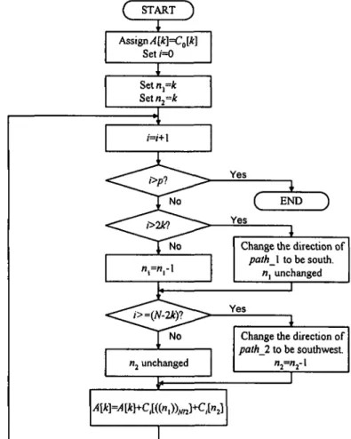
and h[3]a[N-l], h[3]a[l]. Continuing the pro-cess, we illustrate the results in Fig. 4(b). It is only when path_\ encounters the wall that then it changes its regular direction to the south, and vice versa for path_2. The algorithm is summarized as follows.

Algorithm 1. Evaluate A[k]. Step 1. Initialize

Assign A[fc]=C0[&] and set /=0.

Step 2. Sum up all the points located on the two paths toA[k].

Step 2.1) Start path_\ and path_2 from C0[k].

Let the initial directions of path_\ and pathjl be southwest and south, respectively.

Step 2.2) Check the terminal condition of summation.

Increase /by 1. If i>p then stop. Step 2.3) Decide the direction of path_\.

If path_1 is in its current direction traveling to the next point and it is blocked by the wall, then the direc-tion of path_\ will be changed to the south.

Step 2.4) Decide the direction of pathjl. If pathjl is in its current direction traveling to the next point and is blocked by the wall, then the direc-tion of pathjl will be changed to the southwest.

Step 2.5) Add both of the next points on path_\ and pathjl to A[k]. Go back

to Step 2.2).

For example, one can trace the bold solid lines indicated in Fig. 4(b) to evaluate A[2]. Both paths are illustrated encircling the path number. First we

let A[2]=C0[2], and then continuously add all the

points located on these paths together until the paths reach the pth row of matrix C. Path_\ travels

the points, d [ l ] , C2[0], C3[N/2-l], C4[A72-2],

C5[W2-2], ... , and Cp[N/2-2]. This shows that the

direction of path_\ is changed after touching the point

C4[/v72-2]. As for the points on pathjl, which

fol-low the order C,[2], C2[2], C3[2], ..., and Cp[2], the

direction of pathjl is unchanged. To verify this re-sult, substituting k with 2 into Eq. (7) and applying the relations in Eq. (8) and Eq. (9), we get

A[2]=h[-p]a[4+p]+...+h[-l]a[5]+h[0]a[4]+h[l]a[3]+ ...+h[p]a[4-p)

=h[p]a[4+p]+...+h[l]a[5]+h[0]a[4]+h[l)a[3]

=sum of path J2+h[0]a[4]+ sum of path_\. (18) That is the exact result obtained by Algorithm 1.

Note that the direction checking in Algorithm 1 (step 2.3 and step 2.4) is only necessary for a few terms of A[k]. For most of the terms of A [A;], the paths will follow the initial direction all the way until the

Change the direction of

path_\ to be south.

n, unchanged

L

Change the direction of

pathjl to be southwest.

Fig. 6. Flowchart for evaluating A[k\.

end. For A[0], ... , A[p-l], we just have to check the direction of path_\. As for the last Trunc{pl2) terms of A[k], (the Trunc(x) function returns an integer-type value that is the value x rounded toward zero), only the direction checking for path_2 is necessary. Once the direction is changed, the path will follow the new direction and there will be no additional modifica-tions.

Similarly, as shown in Fig. 5(a), a matrix D is used to temporarily record all the possible terms of the nonrepeated products for evaluating B[k]. The (i,n) element in this matrix is defined as

(19) i=l, ..., q+l,n=0, ..., 7W2-1.

To obtain B[k], we follow the steps stated in

Algo-rithm 1 and replace A[k) by B[k], C0[k] by D,[fc-1], p

by q+l, southwest by southeast, and set the initial value of /to 1, respectively. The next point of Dj[m]

on a path is either Di+\[((m+l))N/2\ in the southeast

direction or D,+1[m] in the south direction here. As

with the first example, it is only necessary to check the directions of the paths for just a few coefficients of B[k). Fig. 5(b) shows the corresponding points and the method to calculate each B[k]. The bold solid lines denote the paths for B[2]. One can decompose B[2] by Eq. (7) into several product terms, and use the same approach mentioned in Eq. (18) to verify this result.

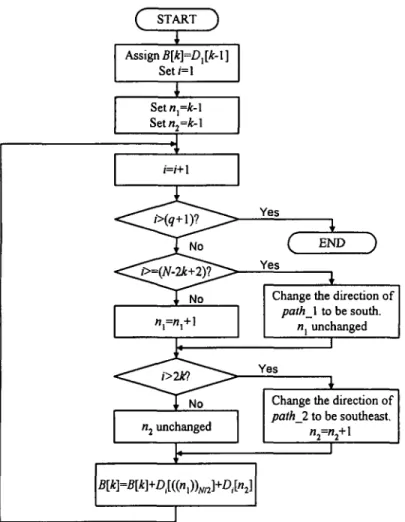
Flowcharts to calculate each A[k] and B[k] are individually shown in Fig. 6 and Fig. 7, respectively.

186 Journal of the Chinese Institute of Engineers, Vol. 22, No. 2 (1999) START ) .!bf;n?.."Vn!. Assign B[k]=Dx[k-\] Set/=1 JJjNlO JTNO 1 J N O n2 unchanged 1 i Yes ( END ) Yes

Change the direction of

path_\ to be south, n, unchanged 1 Yes i »

Change the direction of

path_2 to be southeast.

1

Fig. 7. Flowchart for evaluating B[k].

o[N-l-n] = a()[N-l+n] a(TN-2]a()[N-l]a0[N].

A[l] 0 A[0] 0 A[l] symmetric extension A[k] (a) 0 A[N/2-l]0 A[N/2-l] 0 symmetric extension A[N/2-l-k] = A[N/2+k] a,[-n] = a,[n] a ,rN-l-n] = a JN-l+n] 0 B[l] 0 B[l] 0 symmetric extension (b) B[N/2-l] 0 B[N/2] 0 B[N/2-l] symmetric extension B[N/2+k]-B[N/2-k]

Fig. 8. Filter positions while reconstructing the nth coefficient. (a) filter positions at lowpass channel (b) filter positions at highpass channel.

We treat both ri\ and n2 in these figures as the

col-umns on path_l and pathjl, respectively.

IV. FAST CONVOLUTION ALGORITHM FOR IDWT

We will first discuss how to reconstruct the sequence a[n] from the stored principal terms of A[k] and B[k] by a method similar to the method in Sec-tion III. Later, we will efficiently list all the pos-sible nonrepeated product terms and sum up some of them for each a[n].

Considering the finiteness of the summation of Eq. (6), we can rewrite it to

a[n]=ao[n]+aj[n]

q p + \

= X ti[k]A[(k+n)f2]+ Z g[k]B[(k + n)f2],

k = -q k = -p + 1

for k+n=2l, /eZ, (20)

where g[k] is calculated from Eq. (3). The symmet-ric centers of g[k] and h[k] are at &=1 and at k=0, respectively. Thus, the constraints on these two fil-ters are

h[k]=h[-k] and g[l+k]=g[l-k]. (21)

To calculate a[n] as shown in Eq. (20), first we indi-vidually extend the sequences A[k] and B[k] by Eqs. (10) and (11), respectively, and then upsample them

by interpolating zeros. Next, applying the filters as Eq. (21) to these two sequences, we can obtain the relationship as shown in Eq. (9).

Figure 8(a) denotes the reconstructed sequence from the lowpass channel. According to Eq. (10), the sequence A[k] is a whole-point symmetric exten-sion on the left side, but a half-point symmetric ex-tension on the right side. After the exex-tension, we upsample this sequence by interpolating zeros. Then using the filter, we get

ao[-n]=ao[n] and ao[N-l-n]=ao[N-l+n]. (22)

Similarly, Fig. 8(b) shows the reconstructed sequence from the highpass channel. The sequence B[k] is a half-point symmetry on the left side, and a whole-point symmetry on the right side. Substituting the symmetry filter as shown in Eq. (21) into Eq. (20), we have

a\[-n]=ai[n] and ai[N-l-n]=ai[N-l+n]. (23) With the symmetric property of these two sequences, what we need to do is to calculate the index terms of

ao[n] and ax[n\ at n=0, ..., N-l, and sum them up point

by point to obtain the reconstructed sequence a[n]. To efficiently convolve A[k] and B[k] with fil-ters , we use two matrices E and F to temporarily record all the possible terms of the nonrepeated prod-ucts to reconstruct a[n]. The matrix E stores the products reconstructed from the lowpass channel, and

k= N/2-2 N/2-1 1 N/2-2 N/2-1 E^k E4(k \i EiLk Ejtk Ejfk Eqlk k= EJW Ftl-ik E,M Ej[k] ] hIO]A[O] J h[2]A[0] ] h[4JA[0] kj h[q-l]A[O] ] hIl]A[O] ] h(3]A[0] ] h[5JA|0] ] h[q]A[O] 1 0 JO] « I whole-po * ^ A h[0]A[l] h[2]A[l] h[4]A[l] hlq-.lAm h[l]A[l] h[3]A[l] h[5]A[l] h[q]A[l] 1 ao[2] * tnt symmetry h[0]A[2] h[2]A[2] h[4]A[2] h[q-l]A[2] h[l]A[2] h(3]A[2] h|5]A[2] h[q]A[2] 0 2 •bW ft >< > -h[0]A[3] h[2]A(3] h[4]A[3] h[q-l]A[3] .... h[l]A[3] h[3]A[3] h[5)A[3J h[q]A[3] 0 3 %ra ^«i

X.

^ ^

Fig. 9. Reconstruction of the sequence from the lowpass channel, (a) arrangement of the products (b) corresponding points and the way to calculate each value.

Ffi[k] F,[k] F5[k] g[2]B[l] g[2]B[2] g[2]B[3| g[2]B[4] g[4]B[l] i[4]B[2] g[4]B[3] i[4]B|4] g[6]B[l] i[6]B[2] g[6]B[3] i(6]B[4] g[p]B[l] g[p]B[2] g[p]B[3] g[p]B[4] i(l]B[l] g"[l]B[2] g[l]B[3] i(l]B[4J g(3]B[l] i[3]B[2] g[3]Bt3] i(3]B[4] g[5]B[l] g[5]B[2] g[5]B(3] g[5]B[4] g[2]B[N/2-l] g[2]B[N/2] ~g[4|B[N/2-H .~g[4]B[N/2] ~g[6]B[N/2-U " g[p]B[N/2-l] g(p]BfN/21 g[l]B[N/2] ~g[3]B[N/2-l] lg[3]B[N/2] ~g[5]B[N/2-l] ~g[5]B[N/2] g[p+l]B[2] g[p+l]B[3] g[p+l]B[4] g[p+l]B(N/2-l] g[p+l]B[N/2] k= 0 0 I (a) 2 3 N/2-2 N/2-1 N/2-2

half-point symmetry whole-point symmetry (b)

Fig. 10. Reconstruction of the sequence from the highpass chan-nel, (a) arrangement of the products (b) corresponding points and the way to calculate each value.

the matrix F keeps the products reconstructed from the highpass channel. The (i,k) element of these two matrices is individually defined as:

Ei[k]=h[i]A[k], i=0, ..., q, k=0, -l, (24) and

Fi[k]=g[i]B[k+l], i=0, ..., p+l, k=0, ..., N/2-1, (25)

Figures 9(a) and 10(a) list the elements in these two matrices, respectively. Fig. 9(b) and Fig. 10(b) show the corresponding points and the way to calcu-late each reconstructed value. We assume that p is even and q is odd in these figures for simple illustra-tion. However, there are no constraints on p and q in our design. To calculate the even terms of a[n], we will unite the even terms of ao[n] and a\[n\. The

se-quence ao[n] is obtained by summing up the elements

in the matrix E while the sequence a^[n] is given from

the matrix F. To evaluate the even terms of ao[n],

we assign E0[n] to ao[2n] and then add together all

the points located on the two paths to ao[2n]. These

paths travel in the even-index rows of matrix E. As shown in Fig. 9(b), these two paths independently travel in the southwest and southeast directions. The

elements in matrix E are extended by the whole-point symmetry on the left side, and by the half-point sym-metry on the right side. As a result, one can easily add all the points on the paths without changing di-rections. For simplicity, these paths start with the same point EQ[U\ and will terminate at the largest

even-index row of matrix E. The initial point, E0[n],

does not need to be added to ao[2n] again. To

calcu-late the even terms of ci\[n\, we have to sum up all the points on the two corresponding paths that travel in the even-index rows of matrix F. As shown in Fig.

10(b), these two paths start with F2[n-\] and F2[n]

for G|[2n], then go southwest and southeast, respec-tively. To maintain the directions of the paths, the elements in matrix F are extended by the half-point symmetry and by the whole-point symmetry on the left side and on the right side, individually. Figure 11 illustrates the complete flowchart to calculate the even terms of a[ri\.

Similarly, to evaluate the odd terms of a[n], we

have to add the odd terms of ao[n] and ax[ri] together.

The odd terms of ao[n] are obtained from the

odd-index rows of matrix E while the odd terms of «)[«] are found in the odd-index rows of matrix F. One can follow an approach similar to the one in the last paragraph to acquire the odd terms of a[n]. The

188 Journal of the Chinese Institute of Engineers, Vol. 22, No. 2 (1999)

( START )

Fig. 11. Flowchart of evaluating the even terms of the recon-structed sequence a[n]

flowchart is shown in Fig. 12.

Note that k\ and k2 in Fig. 11 and Fig. 12 are

used to denote the columns on path_\ and path_2, respectively.

V. COMPUTATIONAL COMPLEXITY Assume that the size of an image is N by N. We perform a one-dimensional DWT on the rows and columns of the image. Thus, we have to execute the DWT up to 2N times. For an Appoint circular convo-lution, it requires N multiplication operations to evaluate each transformed coefficient. As a result,

the NMOs taken in a row will be equal to N2. Thus,

the total NMOs are 2N3 for a one scale DWT. For the

next scale, the value of N is reduced by one half. The

NMOs turn out to be 2JV3+2(A72)3 for a 2-scale DWT.

Consequently, for ,s-scale DWT, the total NMOs are up to

2(N/2l~ ' )3 = 16(1 - 2~3s)N3/7 . (26) For regular convolution, it takes 2p+l and 2q+l multiplication operations to calculate each A[k] and B[k], respectively. Then the NMOs for a row equal to be (2p+l)N/2+(2q+l)N/2=(p+q+l)N. Thus, the

regular convolution will demand 2(p+q+l)N2

multi-plication steps for a one scale DWT. Advancing to the next scale, N is reduced by one half but the NMOs for each A[k] and B[k] are unchanged. So the num-ber of multiplication operations for an s-scale DWT will be

. (27)

Table 1. The comparison of computational compolexity among yV-point circular con-volution, regular convolution and the proposed fast convolution with image size N by N (Pixels), s-Scale DWT,

Convolution The number of

multiplication operations N-point circular convolution Regular convolution Fast convolution S(p+q+l)(l-2-2s)N2/3 4(p+q+2)(l-2-2s)N2/3

Fig. 12. Flowchart of evaluating the odd terms of the reconstructed sequence a[n]

Since our fast convolution algorithm omits the computations on the repeated products, the NMOs of the convolution are the sum of the total elements in matrices C and D for a row of an image. That is, (p+\)N/2+(q+l)N/2=(p+q+2)N/2. For the next scale, N is reduced by one half but the NMOs for each A[k] and B[k] are unchanged. Thus, this new convolution will take

(p+q+ 2)(A72'-')2 = 4(p + q -2~2s)N2/3 (28)

1 = 1

multiplication operations for an 5-scale DWT. Com-paring Eq. (27) with Eq. (28), we see that the NMOs have been reduced nearly to one half. Table 1 lists the comparison of computational complexity among these three convolutions.

VI. NUMERICAL RESULTS

To compare the performance of symmetric and

A

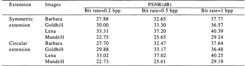
Table 2. The Performance comparison of the symmetric extension and the circular extension in the im-age edges using the EZC coder.

Extension Symmetric extension Circular extension Images Barbara Goldhill Lena Mandrill Barbara Goldhill Lena Mandrill Bit rate=0.2 bpp 27.88 30.00 33.31 22.75 27.70 29.88 33.02 22.73 PSNR(dB) Bit rate=0.5 bpp 32.65 33.30 37.20 25.65 32.47 33.17 37.02 25.61 Bit rate=l bpp 37.77 36.57 40.39 29.24 37.64 36.48 40.25 29.19

circular extensions of an image, we used our previ-ous study, the enchancing zerotree coding (EZC) (Wu and Su, 1998), to test four images, namely Barbara, Goldhill, Lena, and Mandrill. The EZC coder achieved fairly good results for image compression due to the following three reasons. First, the EZC uses a content-dependent scheme to decompose subbands such that the transformed coefficients get closer to zero. Second, the EZC applies a flag at each subband to denote whether all the coefficients in this subband should be encoded corresponding to the cur-rent quantizer. Finally, the optimal compensations on the retrieved coefficients are performed in the EZC coder. All the test images used in this section were 8 bpp, and 512x512. These images can be obtained at the URL, http://links.uwaterloo.ca/greyset2.base.html site.

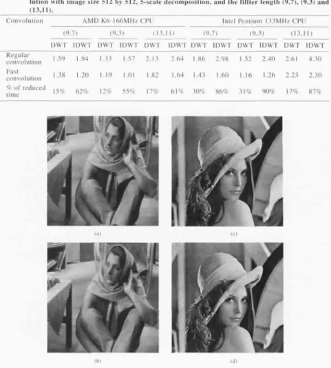
Table 2 shows the coding results from applying the EZC coder to these test images at various bit rates. Both the symmetric extension and the circular extension are reported for comparison. We utilized the 9/7-tap filter (Antonini et al., 1992) for this coder. As shown in Table II, the performance of the symmetric extension is superior to the cir-cular extension. The former can improve the perfor-mance, achieving 0.1 to 0.29 dB for most images. Some reconstructed images for these two extensions are shown in Fig. 13. Although there is no percep-tible difference between these two extensions, one still can use the symmetric extension to avoid possible jumps at the transformed coefficients. Note that the reported bit rates are calculated from the actual compressed files and the PSNRs are from the reconstructed images given by the decoding algorithm. This coder is available by using an anony-mous ftp to cc.nctu.edu.tw under the directory pub/EZC.

To exhibit the improvement in CPU time, both the regular convolution and our new convolu-tion algorithms were tested on two IBM com-patible personal computers (PC). One PC was

equipped with an AMD K6-166 MHz CPU and the other was equipped with an Intel Pentium-133 MHz CPU. The results of the average CPU time are listed in Table III. Three pairs of filters 9/7-tap, 9/3-tap (Antonini et al., 1992), and 13/11-tap (Villasenor et al., 1995) were used in our experi-ments. For the PC with the AMD CPU, the fast con-volution algorithm can increase the execution time up to at least 12% and 55% while executing DWT and IDWT, respectively. However, it can achieve at least a 17% improvement for DWT and an 86% im-provement for IDWT using the PC equipped with the Intel CPU. All of the execution time results point out that the proposed algorithm can reduce the trans-form time. The test programs were written in object-Pascal language Delphi 3.0. Of course, one can further reduce the execution time by the assembly language.

VI. CONCLUSION

In this paper, a fast convolution algorithm for DWT/IDWT was proposed. This algorithm focused on the odd length symmetric filters and the symmet-ric extension of an image. The aim of this paper was to reduce the transform time, which is the essential problem for many wavelet-based image processing al-gorithms. The proposed algorithm can decrease the number of multiplication operations by nearly one half according to the mathematical analysis on the computational complexity. Converting it to a real pro-gram, we can speed up both the DWT and IDWT to at least 12% and 55%, respectively. The most attrac-tive feature of the new algorithm is its simplicity in its final form. The proposed structure can be easily implemented in the hardware design for image or video compression systems.

ACKNOWLEDGMENT

This work was supported by National Science

Journal of the Chinese Institute of Engineers, Vol 22. No. 2 (1999!

Table 3. Mir comparison of average CPU time (sec) of regular convolution and the proposed fast convo-lution with [mage Size 51 2 h> 512. 5-SCaie decomposition, and the t'illter length 19.7|, (9,3) and

Convoluiioii A M I ) K h - l h h M H / CPU Intel Pentium l.UMH/ CPU

19.71 19.3) (13,1 0.7) (9,3) ( 1 3 , 1

DWT IDWT DWT IDWT DWT IDWT DWT 1DWT DWT IDWT DWT iDWT

Regular convolution Fast convolution ' I of reduced lime 33 1.57 2.13 2.64 1.86 1M 1.52 2.40 2.61 4.30 1.38 1.20 1.19 1.01 1.82 1.64 I .43 1,60 1,16 1.26 2.23 2.30 I v , (,:-, I : • , 55( i 17', 6 1 8 3 0 $ S(/,f 31 '/< WV'i 11<Y( K7'/.

Fij 1 ( I hi- comparison o! the reconstructed images ui the BJ ntowti t< extension and ihc circular extension at bii ralt=OJ5 hpp. (a) Barbara.

symmetric extension, and I'SNK- '2 (o ilB (b) Barbara, circuloi extension, and PSNR»32.47 JH. [c) Lean, symnKtrit extensioQ,

and PSNR=37.20 dfi (d) l ena, drculwr extension, and PSNR-.i7.i)2 .IB.

Council of ihc ROC under Granl NSC 87-2213-E-009-043.

NOMENCLATURE

input set|uGncG

flotw] reconstructed sequeace ai Lowpass chan-nel

ii\\n\ reconstructed sequence ai tiigbpass

channel

A \ h \ ouipui transformed sequence at lowpsss

channel

B[k] CM

DM

output transformed sequence at highpass channel

temporary matrix used to store all the possible product terms for evaluating Aik]

temporary matrix used to store all the possible product terms for evaluating

•B[k]

temporary matrix used to store all the possible product terms for evaluating

aoin]

temporary matrix used to store all the possible product terms for evaluating a\[n]

analysis highpass filter synthesis highpass filter analysis lowpass filter synthesis lowpass fitler n modulo N

round x near zero REFERENCES

1. Antonini, M., Barlaud, M., Mathieu, P., and Daubechies, I., 1992, "Image Coding Using Wavelet Transform," IEEE Trans. Image

Process-ing, Vol. 1, pp. 205-220.

2. Sullivan, G., 1988, "Draft Text of Recommenda-tion H.263 Version 2 ("H.263+") for Decision". 3. Martucci, S.A., Sodagar, I., Chiang, T., and Zhang, Y.-Q., 1997, "A Zerotree Wavelet Video Coder," IEEE Trans. Circuits and Systems for

Video Technology, Vol. 7, No. 1, pp. 109-118. 4. Martucci, S.A., 1994 "Symmetric Convolution

and the Discrete Sine and Cosine Transforms," IEEE Trans. Signal Processing, Vol. 42, No. 5, pp. 1038-1051.

5. Oppenheim, A.V. and Schafer, R.W., 1989,

Discrete-Time Signal Processing. Englewood Cliffs, NJ: Prentice Hall.

6. Pennebaker, W.B. and Mitchell, J.L., 1993, JPEG-Still Image Data Compression Standard. New York, NY: Van Nostrand Reinhold.

7. Said, A. and Pearlman, W.A., 1996, "A new, Fast, and Efficient Image Codec Based on Set Partitioning in Hierarchical Trees," IEEE Trans. Circuits and Systems for Video Technology, Vol. 6, no. 3, pp.243-250.

8. Shapiro, J.M., 1993, "Embedded Image Coding Using Zerotrees of Wavelets Coefficients," IEEE Trans. Signal Processing, Vol. 41, pp. 3445-3462. 9. Strang, G. and Nguyen, T., 1996, Wavelets and

Filter Banks. Wellesley MA.

10. Vetterli, M. and Kovacevic, J., 1995, Wavelets and Subband Coding. Englewood Cliffs, NJ: Prentice Hall.

11. Villasenor, J.D., Belzer, B., and Liao, J., 1995, "Wavelet Filter Evaluation for Image Compres-sion", IEEE Trans. Image Processing, Vol. 4, No. 8, pp. 1053-1060.

12. Wu, B.-F. and Su, C.-Y., 1998, "Low Computa-tional Complexity Enhancing Zerotree Coding for Wavelet-based Image Compression," submitted to Signal Processing: Image Communication. 13. Xiong, Z., Ramchandran, K., and Orchard, M.T.,

1997, "Space-frequency Quantization for Wave-let Image Coding," IEEE Trans. Image Process-ing, Vol. 6, no. 5, pp. 677-693.

Discussions of this paper may appear in the discus-sion section of a future issue. All discusdiscus-sions should be submitted to the Editor-in-Chief.

Manuscript Received: Aug. 19, 1998 and Accepted: Sep. 22, 1998

192 Journal of the Chinese Institute of Engineers, Vol. 22, No. 2 (1999)

flsl ^

#cW»fM5£ ' 1£ RlMnifc DWT fP IDWT ^J#lfT^?'JM^ 12% fP 55% fftU