Received March 31, 1999; revised June 16 & July 27, 1999; accepted September 20, 1999. Communicated by Shang-Rong Tsai.
*This work was supported in part by the NSC of the ROC under Grant No. NSC87-2213-E-009-023. A preliminary version of this paper, entitled “IPLS: An Intelligent Parallel Loop Scheduling for Multiprocessor Systems,” ap-peared in Proceedings of the 1998 International Conference on Parallel and Distributed Systems (ICPADS ’98), Taiwan, pp. 775-782, 1998.
169
An Intelligent Parallel Loop Scheduling for
Parallelizing Compilers
*YUN-WOEI FANN, CHAO-TUNG YANG+,
SHIAN-SHYONG TSENGAND CHANG-JIUN TSAI
Department of Computer and Information Science National Chiao Tung University
Hsinchu, Taiwan 300, R.O.C. +ROCSAT Ground System Section
National Space Program Office Hsinchu, Taiwan 300, R.O.C.
In this paper we propose a knowledge-based approach to solving loop-schedul-ing problems. A rule-based system, called IPLS, is developed by combinloop-schedul-ing a reper-tory grid and an attribute ordering table to construct a knowledge base. IPLS chooses an appropriate scheduling algorithm by inferring some features of loops and assigning parallel loops to multiprocessors to achieve significant speedup. Because more at-tributes are proposed, the accuracy of selection of an appropriate scheduling method is improved. In addition, the refined IPLS system can automatically adjust the attributes in the knowledge base according to profile information; therefore, IPLS has the capability of feedback learning. The experimental results show that our approach can achieve greater speedup on multiprocessor systems than can others.
Keywords: parallelizing compiler, parallel loop scheduling, knowledge-based system, multi-processor systems, speedup
1. INTRODUCTION
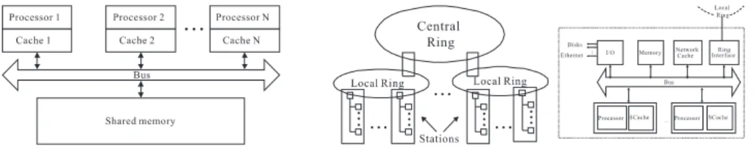
Parallel processing has been one of the most important technologies in modern com-puting for several decades. Many powerful multiprocessor hardware systems have been built to exploit parallelism for concurrent execution. Two models are classified below according to their memory organization, addressing schemes, and inter-processor com-munication mechanisms:
∑ The uniform memory access (UMA) model: Most UMA systems as shown in Fig. 1(a)
are shared-memory environments, in which all processors use the common memory and have equal time to access all memory words.
∑ The non-uniform memory access (NUMA) model -In NUMA system shown in Fig. 1
(b), the cost of accessing memory increases with the distance between the accessing processor and target memory.
In view of the difference between these two architectures, the memory access and interprocessor communication overheads should be taken into consideration when access-ing the shared variables. To speed up multiprocessor systems, it is likely that tasks must be decomposed into several sub-tasks and executed in parallel on different processors. Parallelizing compilers and parallel programming tools that can translate ordinary pro-grams into parallel codes have been proposed. Parallelizing compilers can analyze se-quential programs to detect hidden parallelism. The information is used to automatically restructure sequential programs into parallel sub-tasks for multiprocessors using schedul-ing algorithms. Therefore, it is important to design and implement efficient parallelizschedul-ing compilers that can extract the maximum amount of parallelism for multiprocessors.
An efficient approach to extracting potential parallelism is to concentrate on the parallelism available in the loops. Since the body of a loop may be executed many times, loops often comprise a large portion of a program’s parallelism. By definition, a loop is called a DOALL loop if there is no cross-iteration dependence in the loop; i.e., all the iterations of the loop can be executed in parallel. If all the iterations of a DOALL loop are distributed among different processors as evenly as possible, a high degree of parallelism can be exploited. Parallel loop scheduling is a method that schedules a DOALL loop on multiprocessor systems as evenly as possible.
In a shared-memory multiprocessor system, scheduling decisions can be made ei-ther statically at compile-time or dynamically at runtime. Static scheduling is usually applied to uniformly distributed iterations on processors [1, 2, 4-6, 9-11, 14, 19-21]. However, it has the drawback of creating load imbalances when the loop style is not uni-formly distributed, when the loop bounds cannot be known at compile-time, or when local-ity management cannot be exercised. In contrast, dynamic scheduling is more appropriate for load balancing; however, the runtime overhead must be taken into consideration. In general, parallelizing compilers distribute loop iterations by using only one kind of sched-uling algorithm, which maybe static or dynamic. However, a program may have different loop styles, including a uniform workload, an increasing workload, a decreasing workload, and a random workload. Every scheduling algorithm can achieve good performance with some loop styles and different system states because the loop style and the system envi-ronment influence the selection of scheduling strategies. For example, it is not appropri-ate to apply GSS on a NUMA system because the communication cost of accessing remote memory is too high.
The scheduling performance of a DOALL loop on shared-memory multiprocessor systems is usually dependent upon the amounts of overhead that arise from four main factors: load imbalances among processors, the synchronization overhead, the communi-cation overhead, and the thread management overhead. They are described as follows:
∑ Load imbalances: If some processors are idle, we cannot take full of advantage of their
multiprocessing capacity. A good scheduling algorithm tries to spread the workload around to multiprocessor systems as evenly as possible. To avoid uneven assignment of work units to processors, many loop-scheduling algorithms use a central work queue for remainder iterations.
∑ Synchronization overhead: This type of overhead arises from simultaneous accesses
made by different processors of a set of shared variables that contain the iteration indices.
∑ Communication overhead: This is non-uniform data access time among
multiproces-sor systems and is often caused by having to access remote memory for non-local data. Data locality management policies attempt to minimize the communication over-head by allocating iterations close to their data.
∑ Thread management overhead: This refers to the time required to create, detach and
schedule multiple concurrent lightweight processes to express the concurrency on multithreaded operating systems. It is well known that the system performance will drop if too many threads are created for execution.
It is difficult to balance the tradeoff among these factors; therefore, this paper con-centrates on how to distribute parallel loop iterations on a shared-memory multiprocessor system not only as evenly as possible, but also with the lowest overhead. For example, the block size should be large enough to reduce the synchronization overhead, but load imbal-ance and the communication overhead may become extreme. As described above, none of the scheduling algorithms is best for all cases. That is, all of the algorithms are only appropriate for some cases, and none can manage all these features well. Therefore, find-ing a good trade-off among them is not an easy task. Suppose the parallelizfind-ing compiler can analyze loop attributes, such as the loop style, loop bound, data locality, etc.; an appro-priate scheduling algorithm for this particular case can be determined. This leads to se-lecting scheduling algorithms based on a knowledge-based system approach.
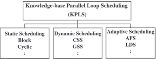
The scheme proposed in [19] is called Knowledge-Based Parallel Loop Scheduling (KPLS). KPLS uses knowledge-based techniques to select an adequate loop-scheduling algorithm for a loop according to the attributes of the loop behaviors and system states. However, in KPLS, some attributes that influence the accuracy of selecting an adequate loop-scheduling algorithm are neglected. Therefore, in this paper, we propose a new approach, called the Intelligent Parallel Loop Scheduling (IPLS) algorithm. It considers more attributes so as to make up for the shortcoming of KPLS. IPLS also integrates more existing loop-scheduling algorithms than KPLS does for UMA and NUMA systems to make good use of their advantages in loop parallelism. Because more attributes are proposed, the accuracy of selection of an appropriate scheduling method is improved. In addition, the refining system in IPLS can automatically adjust the attributes in the knowledge base ac-cording to profile information. Therefore, it has a feedback-learning mechanism. The experimental results show that our approach can achieve more speedup on multiprocessor systems than others can. Furthermore, our approach is obviously superior to others in terms of system maintenance and extensibility. Once a new scheduling algorithm or tech-niques is proposed, it can be easily integrated into IPLS by adding knowledge and rules to improve the power of IPLS.
2. BACKGROUND
The major source of parallelism in a program is loops. If the loop iterations can be distributed to different processors as evenly as possible, the parallelism within loop itera-tions can be exploited. Parallel loop scheduling is used to achieve this goal by determin-ing how to assign the DOALL loops onto each processor in a balanced fashion so as to effect a high level of parallelism with the least amount of overhead. In a shared-memory multiprocessor system, two kinds of parallel loop scheduling decisions can be made either statically at compile-time or dynamically at run-time. In the rest of this section, we will review the various scheduling algorithms. We use N and P to denote, respectively, the number of iterations and the number of processors, and we set the size of the ith partition to
Ki.
2.1 Static Scheduling
Static scheduling [6] makes a scheduling decision at compile-time and uniformly
distributes loop iterations onto processors. It is applied when each loop iteration takes roughly the same amount of time, and the compiler knows how many iterations must be run and how many processors are available for use at compile-time. It has the advantage of incurring the minimum scheduling overhead, but load imbalances may occur. However, static scheduling may perform unacceptably when the loop style is not uniformly distrib-uted or the loop bounds can not be known at compile-time. In the following, the different static scheduling methods with and without consideration of data locality are reviewed.
Block Scheduling In block scheduling [6], N iterations are divided into
NP rounds.Each round consists of consecutive iterations and is assigned to one processor. This is only suitable for uniformly distributed loop iterations.
Cyclic Scheduling Instead of assigning to a processor a consecutive block of iterations,
iterations are assigned to different processors in a cyclic fashion [6]; i.e., iteration i is assigned to processor i mod P. This method may produce a more balanced schedule than block scheduling for some non-uniformly distributed parallel loops.
Block-D Scheduling In NUMA systems, managing data locality is important due to the
increased cost of accessing remote memory. For good performance, it is essential that the loop partitioning match the data partitioning. If both the data partitioning and loop sched-uling occur in blocks, the static schedsched-uling is called Block-D schedsched-uling [6].
Cyclic-D Scheduling As mentioned above, if both the data partitioning and loop
schedul-ing occur in a cyclic fashion, the static schedulschedul-ing is called Cyclic-D schedulschedul-ing [6].
2.2 Dynamic Scheduling
Dynamic scheduling adjusts the schedule during execution whenever it is uncertain
how many iterations to expect or when each iteration will take a different amount of time due to a branching statement inside the loop. Although it is more suitable for load balanc-ing between processors, runtime overhead and memory contention must be considered.
Dynamic scheduling algorithms, such as SS [12], fixed-size chunking [3, 11], GSS [8], factor-ing [2], and TSS [11], share the followfactor-ing same characteristics. They always maintain a global queue containing indices of iterations. At runtime, when a processor is idle, it issues syn-chronous operations to the global queue and fetches some iterations for execution.
Pure Self-Scheduling (SS) This is the easiest and most straightforward dynamic loop
scheduling algorithm [12]. Whenever a processor is idle, an iteration is allocated to it. This algorithm achieves good load balancing but also introduces excessive overhead.
Chunk Self-Scheduling (CSS) Instead of allocating one iteration to an idle processor as
in self-scheduling, CSS allocates k iterations each time, where k, called the chunk size, is fixed and must be specified by either the programmer or the compiler [3, 11]. When the chunk size is one, this scheme is pure self-scheduling, as discussed above. If the chunk size is set to the bound of the parallel loop equally divided by the number of processors, the scheme becomes static scheduling. A large chunk size will cause load imbalancing while a small chunk is likely to produce too much scheduling overhead. For different partitioning schemes, we adapted CSS/l, which is a modified version of CSS, where l means the number of chunks.
Enhanced Chunk Self-Scheduling (ECSS) When all the dependent iterations of a loop
are assigned to the same processor, the dependent relation is satisfied and it does not need synchronization operations to keep the executing order of the loop. Let chunk size be K. If a loop exist loop carried dependence distance D, and if every time each processor gets K iterations that mutually are a distance D from work queue, then the dependent relation of K iterations are reserved without a synchronization operation. For the loop whose LCD distance is larger than one, ECSS can develop more parallelism than CSS and reduce the amount of synchronization overhead.
Guided Self-Scheduling (GSS) This algorithm can dynamically change the number of
iterations assigned to each processor [8]. More specifically, the next chunk size is deter-mined by dividing the number of remaining iterations of a parallel loop by the number of available processors. The property of decreasing chunk size implies an effort is made to achieve load balancing and to reduce the scheduling overhead. By allocating large chunks at the beginning of a parallel loop, one can reduce the frequency of mutually exclusive ac-cesses to shared loop indices. The small chunks at the end of a loop partition serve to balance the workload across all the processors.
Multilevel Interleaved Guided Self-Scheduling (MIGSS) This is a hybrid scheduling
scheme blended with run-time scheduling techniques and compile-time loop restructuring [15]. Its run-time scheduling is based on guided self-scheduling. A compile-time loop transformation method is used to enhance the parallel execution performance. The basic idea of MIGSS is to split a hybrid perfectly nested loop into several independent loops and then apply high-level spreading to the generated loops. Since the resulting loops are independent, loop splitting must be applied to outer DOALL loops only. As in the GSS scheme, loop interchange and loop coalescing can be applied to the resulting loops to reduce the number of synchronization points.
Factoring In some cases GSS might assign too much work to the first few processors, so that
the remaining iterations are not time-consuming enough to balance the workload. This situation arises when the initial iterations in a loop are much more time-consuming than later iterations. The factoring algorithm addresses this problem [2]. The allocation of loop iterations to processors proceeds in phases. During each phase, only a subset of the remaining loop iterations (usually half) is divided equally among the available processors. Because Factoring allocates a subset of the remaining iterations in each phase, it balances loads better than GSS does when the computation times of loop iterations vary substantially. In addition, the synchronization overhead of Factoring is not significantly larger than that of GSS.
Trapezoid Self-Scheduling (TSS) This approach tries to reduce the need for
synchroni-zation while still maintaining a reasonable load balance [11]. TSS(Ns, Nf) assigns the first
Ns iterations of a loop to the processor starting the loop and the last Nf iterations to the
processor performing the last fetch, where Ns and Nf are both specified by either the
pro-grammer or the parallelizing compiler. This algorithm allocates large chunks of iterations to the first few processors and successively smaller chunks to the last few processors. Tzen and Ni proposed TSS(N/2P, 1) as a general selection. In this case, the first chunk is of size 2NP, and consecutive chunks differ in size N
P
8 2 iterations. The difference in the size of successive chunks is always a constant in TSS whereas it is a decreasing function in GSS and in Factoring.
Self-Adjusting Scheduling (SAS) Hamidzadeh and Lilja introduced the SAS technique,
which is capable of improving the performance of programs on NUMA systems by em-ploying an on-line optimization technique on a dedicated processor [1]. The object of this algorithm is to address the tradeoffs between three interrelated factors in dynamic scheduling, namely the remote memory access delay, load imbalancing, and scheduling costs, to compute schedules that result in minimum total loop execution times on a multi-processor system. SAS is an on-line branch-and-bound algorithm that searches through a space of all possible partial and complete schedules. The overlapping scheduling and execution, along with self-adjustment of the durations of partial scheduling periods re-duces scheduling and synchronization costs significantly. To satisfy load balancing and locality management, SAS introduces a unified cost model that accounts for both of these factors simultaneously.
Safe Self-Scheduling (SSS) The basic idea behind SSS is to assign to each processor the
largest number, m, of consecutive iterations having a cumulative execution time just ex-ceeding the average processor workload EP [5]; i.e., i s
s m i s s m e i E P e i =+ − < =+ ∑ 1 < ∑ ( ) ( ), where E i e i N
= ∑ =1 ( ) and s is some starting iteration number of the chore. m is the best choice of chore size, which is the smallest critical chore size. SSS is similar to Factoring but im-proves the shortcoming of Factoring. In the implementation of SSS, α×N
P iterations are
given to each processor at compile time, where 0 < a £ 1. (For most of the applications we
have encountered, 0.5 £ a < 1.) At run time, an idle processor fetches more unscheduled
iterations. The ith fetching processor is assigned a chunk of max
{
(
1−α)
Pi ×N×α,}
P k ,Adaptive Hybrid Scheduling (AHS) One solution to workload imbalance on every processor
is to adopt a hybrid scheduling mechanism. This mechanism distributes the workload as much as possible at compile-time based on not breaking the load balance among all processors, and it schedules the left workload at run time. Let Emax, Emin and Eavg be the maximum, average
and minimum execution times of every iteration, respectively; obviously, E = N × Eavg. A
block is defined as a number of successive iterations. The jth block is denoted as B
j, and the
number of iterations included in Bj is called the block size, denoted as |BSj|. In AHS, the first
block B1 is assigned to processor p1, the second block B2 is assigned to processor p2, and so on. Every m consecutive blocks forms a round. A large number, |BS0| = (N/P) × b + E/(Emax × p) × g = (N/P) × w, of iterations is distributed in round 0, where b is the probability not to
fetch again and g is the probability to fetch again, obviously b + g = 1. b and g are selected by
programmers according to the properties of parallel computers. The other iterations are left for later rounds. |BSi| = (Nr/P) × b + E/(Emax × p) × g = (Nr/P) × w, Nr is the number of remaining
iterations.
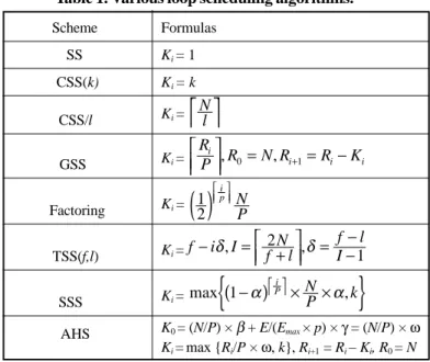
Table 1. Various loop scheduling algorithms.
Scheme Formulas SS Ki = 1 CSS(k) Ki = k CSS/l Ki =
Nl GSS Ki = R P R N R R K i i i i , 0= , +1= − Factoring Ki = 1 2( )
ip N P TSS(f,l) Ki =f i I N f l f l I − = + = −− δ, 2 ,δ 1 SSS Ki = max{
(
1−α)
× ×α,}
i P N P kAHS K0 = (N/P) × b + E/(Emax × p) × g = (N/P) × w
Ki =max {Ri/P × w, k}, Ri+1 = Ri – Ki, R0 = N
Table 2. Sample partition sizes.
Scheme N = 1000 and P = 4 SS 111111111111... CSS(125) 125 125 125 125 125 125 125 125 CSS/4 250 250 250 250 GSS 250 188 141 106 79 59 45 33 25 ... Factoring 125 125 125 125 62 62 62 62 31 ... TSS(88,12) 88 84 80 76 72 68 64 60 ... 12 SSS 188 188 188 188 47 47 47 47 12 12 ... AHS 188 188 188 188 16 16 16 16 11 11 ...
Formulas for calculating Ki in different algorithms are listed in Table 1. Table 2 gives
sample partition sizes for SS, CSS(125), CSS/4, GSS, Factoring, TSS(88, 12), SSS, and AHS, when N = 1000 and P = 4.
2.3 Affinity Scheduling
As modern shared memory multiprocessor systems have high and non-uniform memory access costs, these costs gradually dominate the source of a parallel application’s execution. To reduce the remote memory access cost, affinity scheduling algorithms partition and sched-ule the loop iterations to the local work queue of each processor. The data for iteration is placed on the cache of some dedicated processor to be used repeatedly. Therefore, they are more suitable for a NUMA machine that takes data locality into account, but load balancing between the processors, runtime overhead and memory access rate must be considered.
Affinity Scheduling (AFS) Most of the dynamic loop scheduling methods work well
only in UMA share-memory systems; in NUMA systems, the overhead of communication for accessing remote memory is too heavy and more important. While most existing dy-namic scheduling algorithms fail to take locality into account, there is one method, called AFS [7], that gives us a useful alternative. Markatos and LeBlanc proposed this algorithm, which takes locality into account [7]. AFS consists of two phases: initialization and
execution. In the initialization phase, AFS divides the iterations of a loop into chunks of
size
NP . The ith chunk of iterations is always placed in the local work queue of processori. During the execution phase, when a processor is idle, the processor removes 1k (in general, we assume that k = P) of the remaining iterations from its local work queue and executes them. If a processor’s work queue is empty, the scheduling process finds the most loaded processor, removes
1P of the remaining iterations from that processor’s work queue, and executes them.Modified Affinity Scheduling (MAFS) Because the migration strategy of AFS is too
conservative, a mortified policy called MAFS [13] to fix the migration algorithm has been. The main difference between AFS and MAFS is in the migration policy. MAFS assigns a more appropriate quantum than AFS when migrating work between processors. For an idle processor, instead of taking P1 iterations from the most loaded processor, i, it removes
min(N Ni, i N ) most i 1 − 1 iterations, where Ni 1 equals NPi N i most
, , is the most loaded processor’s remaining iterations, and Ni is the total iterations of all processors at time ti.
This scheme combines the advantages of GSS and AFS, reduces the communication cost, avoids using global queues to alleviate contention, and provides better load balancing.
Locality-Based Dynamic Scheduling (LDS) Most of the loops scheduling methods
work well only in share-memory systems, but in NUMA systems, the overhead of network communication is too heavy and more important. While most existing dynamic scheduling algorithms fail to take locality into account, there is one method called LDS [6] that offers a good solution to this kind of problem. LDS partitions loops into
2nP sub-tasks, wheren is the number of remaining unscheduled iterations. The subtask size is half of GSS, but the
proces-sor p executes a subtask from 1 to S1, then LDS executes the iterations as follows: p + P, p + 2P, ..., p + P × S1. On the other hand, if the data locality is sequential, the subtask will be executed in the p × B + 1, p × B + 2, º, p × B + S1 order, where B is the block size with a number
of continuous iterations. When all the local iterations have been executed completely, non-local iterations are acquired from the processor with the most unscheduled iterations.
Dynamic Partitioned Affinity Scheduling (DAFS) The basic idea behind this approach
is to dynamically change the partitioned size of AFS scheduling by using the traced record of previous executed iterations [10]. There are three distinct phases in this method. First is the loop initialization phase: it partitions iterations with size NP to each processor, and this is only done for the first execution of the loop. Second is the loop execution phase: a processor removes 1P iterations from its local work queue and executes them. If a processor’s local work queue is empty, the idle processor finds the most heavily loaded processor, migrates 1P of the remaining iterations of that processor and executes them. Every processor keeps track of the actual number of iterations that it has executed. The first two steps are the same as in AFS. Third is the re-initialization phase: before executing the next iteration loop, the loop partition for each processor is re-initialized. Each pro-cessor runs the size of iterations, which is last time they were executed. DAFS can dy-namically change the partition size in each processor initialization, and the proposed algo-rithm is more capable of handling workloads that are unbalanced with respect to the amount of computation represented by each iteration.
Clustered Affinity Scheduling (CAFS) A new algorithm called clustered affinity scheduling
(CAFS) has been proposed to improve AFS on cluster NUMA machines [16]. In the initial-ization phase of CAFS, the iterations are divided into C clusters, and a cluster consists of
S P C
= processors, where C is about
P and P is the number of processors, respectively. Processors 1, 2, ..., and C are assigned to clusters 1, 2, ..., and C in sequence, respectively. But processors (C + 1), (C + 2), ..., and 2C are assigned to the clusters in reverse order, and so on.In the execution phase of CAFS, each time, a processor performs
1S of the re-maining iterations from its local queue until the local queue is empty, where S is the number of processors in each cluster. If no imbalance occurs, then migration is not needed. When imbalance occurs, the first idle processor migrates
1S iterations from the proces-sor with the largest number of non-executing iterations in its local cluster. Instead of searching the other P-1 processor of AFS, CAFS searches only the other processors of itscluster.
Localized Affinity Scheduling (LAFS) A new algorithm called localized affinity scheduling
(LAFS) has been proposed to improve AFS on a cluster NUMA machines [17]. In the initialization phase of LAFS, the iterations are divided into NP chunks, where N is the total number of loop iterations and P is the number of processors. If there are C clusters in the NUMA system, then chunk 1, chunk 2, ..., and chunk C are assigned, respectively, to the first
processor of cluster 1, cluster 2, ..., and cluster C in order. Sequentially, chunk C + 1, chunk
C + 2, ..., and chunk 2C are assigned to the second processor of cluster 1, cluster 2, ..., and
cluster C in sequence, and so on.
In the execution phase of LAFS, each time, a processor performs
1S of the remain-ing iterations form its local queue until the local queue is empty, where S is the number of processor in each cluster. If no imbalance occurs, then migration is not needed. When imbalance occurs, the first idle processor migrates
1S iterations from the processor with the largest number of non-executing iterations in its local cluster. If the queues of processors in local cluster are all empty, the idle processor migrates
P1 iterations from the processor with the largest number of non-executing iterations in other clusters.Global Distributed Control Scheduling (GDCS) The basic idea behind GDCS is to
decentralize the scheduling task among all the processors [4]. The scheme logically orga-nizes P processors in a ring topology. Initially, GDCS assigns NP iterations to each pro-cessor using the static scheduling scheme in the hope that each propro-cessor will receive the same size workload. Each processor executes these assigned iterations from its local queue. When a processor Pi becomes idle, it requests extra iterations from successive
processors on the ring, Pi+1, Pi+2, ..., PN, P1, ..., Pi-1, until it finds an active processor that still
has more than b iterations. The active node, processor Pj, dispatches a iterations to this
request, where a and b are two threshold values. The processor Pi remembers that
proces-sor Pj was the last node from which a request was satisfied. The next time Pi becomes idle,
it starts requesting work from processor Pj, by-passing processors between Pi and Pj. An
additional feature of this scheme is that if, in the meantime, processor Pj becomes idle and
processor Pj remembers that it received tasks from processor Pk, then node Pi will jump
from Pj directly to Pk without asking for work from processors between Pj and Pk. Thus, it
can avoid unnecessary task searching overheads.
2.4 Knowledge-Based Approach
There are four aspects to the problem of loop scheduling on shared-memory multiprocessors: the synchronization overhead, communication overhead, threaded man-agement overhead, and load balancing. In order to reduce the synchronization overhead, the block size should be large, but load imbalance and the communication overhead may become very serious. Therefore, finding a good trade off between them is not easy. That is, all of the algorithms are only suitable in some cases, and none can do well in all these four aspects.
A rule-based system, called Knowledge-based Parallel Loop Scheduling (KPLS) [19], was proposed to make use of the advantages of typical loop scheduling algorithms for parallelism. KPLS can choose an appropriate scheduling by analyzing the characteristics of the input program and can apply the selected scheduling to assign parallel loops on multi-processor systems to achieve a high level of speedup.
Because KPLS achieves good performance by selecting an appropriate scheduling algorithm for each executed application, KPLS is very similar to other scheduling algorithms. We show the hierarchy of loop-scheduling algorithms in Fig. 2.
3. A NEW APPROACH TO PARALLEL LOOP SCHEDULING
Suppose the parallelizing compiler can analyze a loop’s attributes, such as the loop style, loop bound, data locality, etc.; a suitable scheduling algorithm for this particular case can be determined. This leads us to select scheduling algorithms by using a knowl-edge-based system approach to get reasonable execution results. Below, we shall propose a new approach which uses knowledge-based techniques to construct an intelligent parallel loop scheduling (IPLS).
In this section, we will further propose two methods to enhance the functionality of IPLS. One includes additional attributes that influence the selection of appropriate sched-uling algorithm for a parallel loop. If there are more attributes that can be used to increase the accuracy of selecting an appropriate algorithm, the functionality of IPLS can be improved. The other is that a refining system, a new component is developed to improve the inferrence accuracy of IPLS.
3.1 Some Attributes Affecting Scheduling Performance
Four main overheads, the processor load imbalances, synchronization overhead, com-munication overhead, and thread management overhead, influence the performance of par-allel loop scheduling on multiprocessor systems. For example, the block size should be large enough to reduce the synchronization overhead, but the load imbalance and commu-nication overhead may become extreme. As described above, there is no scheduling algo-rithm that is best for all cases. That is, all of the algoalgo-rithms are only suitable for some cases, and none can manage all these aspects well. Therefore, finding a trade-off among them is not an easy task. According to the analysis of numerous related researches, eigh-teen attributes influencing the selection of an adequate loop-scheduling algorithm can be classified into three categories: the system architecture, loop information, and scheduling method. They are discussed in detail below.
3.1.1 The attributes of the system architecture
∑ Number of processors: The number of processors must be known at compile time if we
want to use the static scheduling algorithm. This is a necessary condition for static scheduling since a scheduling decision is made at compile time. For dynamic sched-uling methods, except CSS, the factors can be omitted.
∑ Machine model: Because of the difference between UMA and NUMA, the memory
access and inter-processor communication overheads should be taken into consider-ation when accessing shared variables. If a loop has strong data locality, it seems best
Fig. 2. The hierarchy of loop scheduling algorithms.
Knowledge-base Parallel Loop Scheduling (KPLS) Static Scheduling Block Cyclic : Dynamic Scheduling CSS GSS : Adaptive Scheduling AFS LDS :
to adopt a AFS on NUMA system so that the number of remote memory accesses will be reduced. For a well load-balanced loop, we can consider to using CSS on a UMA system so that the synchronization overhead and communication cost can be reduced.
∑ Cache size: When a block of data is retrieved and placed in the cache, not only the
desired word, but also some adjacent words are retrieved. As the block size increases, the hit ratio will at first increase because of the principle of locality: there is great probability that data in the vicinity of a referenced word will be referenced in the near future. As the block size increases, more useful data is brought into the cache. The relationship between the block size and hit ratio depends on the locality characteris-tics of a particular program, and no definitive optimum value has been found.
∑ Memory access rate: The memory access cost for a UMA system and a NUMA
Sys-tem is different because NUMA will spend much more on memory access if the data is missed in cache. When a migration policy is used for AFS, we must set the value of the transfer_limit by considering the memory access rate to avoid unnecessary migra-tion of chunks.
3.1.2 The attributes of loop information
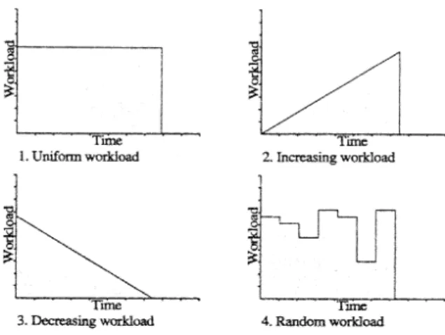
∑ Loop style: Loops can be roughly divided into four kinds as shown in Fig. 3: uniform
workload, increasing workload, decreasing workload, and random workload loops are the most common ones in programs, and should cover most cases. In general, increas-ing workload and decreasincreas-ing workload are called uniform workload loops. The static scheduling method is only suitable for uniform workload loops. In contrast, dynamic scheduling is suitable for all loop styles except that GSS is not good for the third kind. It is possible GSS will initially allocate too many iterations to a processor when the third kind of loop is present; that is, GSS may cause load imbalancing.
∑ Program size: For Enhanced CSS and Factoring, the size of a loop affects the fitness
about the adopted scheduling algorithm. If the size of the loop is large, the performance will be improved.
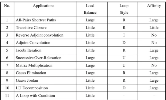
∑ Loop type: The typical applications listed in Table 3 have been studied and implemented
in related researches. Some features of these applications, such as the load balance, loop style and affinity, are different. Therefore, each application listed in Table 3 can be set as a specific type of loop. If the experience used to correctly choose an adequate scheduling algorithm for each loop type can be applied to other programs, then the accuracy of the inference engine in IPLS will be enhanced.
∑ Loop boundary: It is necessary to know the boundary of a loop at compile time before
the compiler applies the static scheduling method so that the synchronization overhead can be reduced. On the other hand, this is not necessary for the dynamic scheduling method because the boundary will be known at runtime.
Table 3. 11 types of loops.
No. Applications Load Loop Affinity
Balance Style
1 All-Pairs Shortest Paths Large R Large
2 Transitive Closure Little R Little
3 Reverse Adjoint convolution Little I No
4 Adjoint Convolution Little D No
5 Jacobi Iteration Little R Large
6 Successive Over-Relaxation Large U Large
7 Matrix Multiplication Large U No
8 Gauss Elimination Large R Large
9 Gauss Jordan Little R Large
10 LU Decomposition Little D Large
11 A Loop with Condition Little – –
∑ Data locality: Among all the scheduling algorithms, only AFS, MAFS, LDS and DAFS
consider data locality. They work well when there is strong data locality in the loop. Strong data locality is common in many applications, particularly those that employ iterative algorithms wherein a parallel loop is nested within a sequential loop. Take the program segment of Successive Over-Relaxation shown in Fig. 4 as an example. The ith iteration of the parallel loop always accesses the ith row of the matrix. Thus
data locality is the only effect that can be exploited.
∑ Loop level: If a loop is nested, usually the level of parallelism is large, especially when a
parallel loop is embedded within a sequential loop. This is because the more the execu-tion times of iteraexecu-tions of outer loop, the more the occurrence of data locality needed by inner parallel loop in the cache of processors on a UMA machine. Usually, the needed data are the elements of the matrix that are at different locations. This is especially
obvious on a NUMA machine. For example, the re-initialization phase in DAFS needs nested loops to dynamically change the partition size, so that it can reassign the workload of each processor as balanced a manner as possible.
3.1.3 The attributes of scheduling method
∑ Start time: If the start times of processors are unequal, static scheduling may not perform
well. In contrast, dynamic methods can work well when this unequal processor start time condition is applied.
∑ Loop carried dependence: The attribute decides if the class of data dependence of a
loop is DOALL or DOACROSS. This will influence the parallelism of the program and an adequate scheduling algorithm must be adopted. When the LCD distance of a loop is larger than one, we can apply ECSS to schedule the loop so as to reduce the synchronization overhead.
∑ Thread overhead: The overhead for creating and executing a thread has to be considered.
Large numbers of threads can balance imbalanced workloads but may introduce an over-head that worsens performance. This is a tradeoff. The results indicate that workloads must be as evenly distributed as possible, and that a minimum number of threads should be used.
∑ Communication cost: In UMA systems, the effect of network overhead has never been
considered. But in NUMA systems, the network traffic exerts a very important influ-ence on the scheduling of decisions. The right decision will save message-passing time and network communication. This attribute has the same effect that data locality has, in that the LDS method is a good example of this kind of problem may be handle. The network communication overhead can be roughly divided into three levels:light traffic, normal traffic and heavy traffic.
∑ Synchronization overhead: The synchronization primitives provided by a system are
related to the synchronization overhead introduced by scheduling algorithms. If a system provides few synchronization primitives, the synchronization overhead will be high. Thus, we divide the synchronization overhead into four levels. Level one is no overhead, level two is slight overhead, level three is moderate overhead, and level four is high overhead. SS works well when there is no synchronization overhead since it may introduce many overheads when shared variables are accessed. GSS does not work well when the overhead is moderate or high.
Fig. 4. The program segment of SOR.
for (i = 1; i <= MAXITERATIONS; i++)//SEQUENTIAL for (j = 1; j <= N; j++)//PARALLEL
for (k = 1; k <= N; k++)//SEQUENTIAL A(J, k) = UPDATE(A, j, k)
∑ Easie of: If two scheduling methods are suitable for a particular loop, the one that is
easier to implement should be chosen. Therefore, ease of implementation should also be considered in our expert system approach.
∑ Factor: In some scheduling strategies, the values of factors, such as allocation factor
in SSS [5], b and g in AHS, the chunk size in CSS, etc, deterministically affect the
execution time of the program. Therefore, they should not be neglected if we want to get optimal factors in order to achieve reasonable performance.
∑ Prefetch: To maximize memory performance, prefetching of multiple single-word
blocks on a miss reduces the miss ratio by approximately 5% to 30% compared to a system with no prefetching. The adaptive prefetching strategy tends to further reduce the miss ratio and the network traffic. In addition, the average memory delay in a multiprocessor system using this adaptive prefetching will be reduced. The relation between a loop-scheduling algorithm and the method used to prefetch the data is not clear and will not be discussed in this paper. The memory performance appears to be relatively insensitive to whether the specific loop-scheduling strategy is GSS, or to whether a single chunk of iterations is assigned to each processor at the start of each parallel loop.
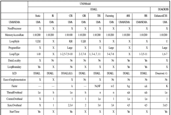
Tables 4 and 5 show the relationships between seventeen attributes and parallel loop scheduling algorithms in UMA and NUMA models, respectively. The features mentioned above are the attributes based upon which we constructed our attribute grid. ‘Machine model’ has two categories: UMA and NUMA. ‘Memory access ratio’ means the speed ratio of the cache, memory and network. ‘CPU number’ denotes the system size, which can be classified into three levels, small, medium, or large. ‘Loop style’ includes four kinds of loops: U(uniform), I(increasing), D(decreasing) and R(random). ‘Program size’ shows the appropriate scale that algorithms fit. ‘Data locality’ determines if loop data behavior has affinity or not. ‘Loop boundary’ determines if it must be known at compile time. ‘Loop level’ determines if a nested loop is profitable to algorithms. ‘Loop carried dependence’ is classified as DOALL and DOACROSS. ‘Ease of implementation’ describes if implementation of the algorithm is easy. ‘Facto’ means the variables, which can dynami-cally influence the performance due to loop information and system states. The overheads of synchronization, communication and thread management are roughly classified into four levels: none, light, normal, and heavy. ‘Start time’ determines whether all each processor starting time need to be equal or not.
3.2 The Anatomy of the IPLS System
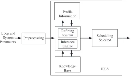
In this paper, we propose a new system, called intelligent parallel loop scheduling (IPLS) (Fig. 5), which uses knowledge-based techniques to select an appropriate loop-scheduling algorithm. The approach makes good use of the advantages of algorithms to improve loop parallelism. By the resulting algorithms for assigning parallel loop on multipro-cessor systems, it is believed that the applications can save execution time and achieve a high level of speedup.
Table 5. The attributive table for NUMA models.
NUMA Model DOALL
AFS MAFS CAFS LAFS DAFS LDS GDCS[4] ASS
UMA/NUMA NUMA NUMA NUMA NUMA NUMA NUMA NUMA NUMA
No of Processor S,M S,M S,M,L S,M,L S S,M S,M S
Memory Access Rate 1:10:200 1:10:200 1:10:200 1:10:200 1:10:200 1:10:200 1:10:200 1:10:200
Loop Style X D,I,R X X X X X X
Program Size — — — X — — — —
Loop Type 2-3, 9-10 2, 4-5 1, 4, 8 1, 4, 8 2, 5, 9, 11 1, 5, 6, 8, 10 2, 5, 9, 11 2, 4, 5, 6
Data Locality Yes Yes Yes Yes Yes Yes Yes Yes
Loop boundary X X X X X X Yes X
Loop Level X X X X X X X X
LCD DOALL DOALL DOALL DOALL DOALL DOALL DOALL DOALL
Ease of implementation No No No No No No No No
Factor 0.5<a<1 — k K — b a,b A=pN2
Thread Overhead l, n l l,n l,n l l,n l,n l
Comm. Overhead l l l l l l,n,h l,n,h h
Sync. Overhead 3, 4 5 3,4 3.4 5 3,4 4,5 3,4
Start Time X X X X X X X X
Table 4. The attributive table for UMA models.
UMA Model
DOALL DOACROSS
Static SS CSS GSS TSS Factoring AHS SSS Enhanced CSS UMA/NUMA UMA UMA UMA UMA UMA UMA UMA/NUMA UMA/NUMA UMA
No of Processor X X X X X X X X X
Memory Access Rate 1:10:200 1:10:200 1:10:100 1:10:200 1:10:200 1:10:200 1:10:200 1:10:200 1:10:200
Loop Style U,D,I X R,R U,I,R X X X X U
Program Size X X Large X X Large X X Large
Loop Type 1-10 X 1-2, 5-7, 9-10 2-3, 7-8 1, 3-4, 7, 11 3-4, 7-8 X 1-3, 5-11 1, 6-7
Data Locality X No No No No No Yes Yes X
Loop Boundary Yes X No X X X Yes Yes X
LCD DOALL DOALL DOALL(0,1) DOALL DOALL DOALL DOALL DOALL Doacross (>1)
Ease of implementation X X X No X No No No No
Factor — — k — Ns, NF x=2 b,g a,k K
Thread Overhead l,n h l,n h n n n,h n,h l,n
Comm. Overhead X l l l l,n l l,n l,n l
Sync. Overhead X 1 2,3,4 2 3,4 3,4 4,5 4,5 3,4,5
A knowledge system is a system that depends on a vast base of knowledge to perform difficult tasks. The knowledge is saved in a knowledge base separate from the inference component. This makes it convenient to append new knowledge or update existing edge easily. The rule-based approach is one of the forms commonly used in many knowl-edge-based systems. The primary difficulty in building a knowledge base is in acquiring the desired knowledge. To ease acquisition of knowledge, one popular technique is Reper-tory Grid Analysis (RGA). RGA is easy to use, but it suffers from the problem of missing embedded meanings. For example, when a doctor says that the symptoms of cold are headache, coughing and sneezing, he may have those symptons. However, in RGA, a per-son is not considered to catch a cold unless that he has all of the symptoms. To overcome the problem, the concept of Attribute Ordering Table (AOT) is employed to elicit embed-ded meanings by recording the importance of each. A knowledge-based system is com-posed of two parts: the development environment and the runtime environment. The former is used to build the knowledge base while the latter is used to solve the problem. In this paper, the development environment is not discussed. The runtime environment contains five components, which are briefly described as follows:
∑ Knowledge Base: This component contains knowledge required to solve the problem of
determining an appropriate parallel loop-scheduling algorithm to be applied. The knowl-edge is constructed as a rule base. This type of system uses knowlknowl-edge encoded in the form of production rules, i.e., If ... Then ... rules.
∑ Inference Engine: The inference engine is the interpreter of the knowledge stored in the
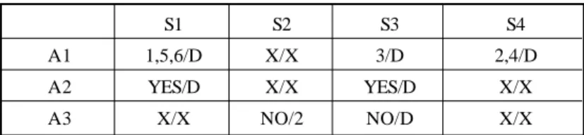
knowledge base. It examines the contents of the knowledge base and the data, includ-ing the system characteristics and the loop attributes, provided by the machine architec-ture and programmers to draw a conclusion, an appropriate parallel loop-scheduling algorithm. The inference engine attempts to find connections between the input at-tributes explained in section three and the selected loop-scheduling algorithm accord-ing to RGA and AOT. An example of applyaccord-ing RGA/AOT is shown in Table 6. ‘X’ means
Fig. 5. The system architecture of IPLS.
Loop and System Parameters Preprocessing Profile Information Refining System Inference Engine Knowledge Base Scheduling Selected IPLS
that the attribute has no relation with the scheduling algorithm. ‘D’ means that the attribute dominates the scheduling algorithm; i.e., if the attribute is not equal to the entry value, it is impossible to apply the scheduling algorithm. For those entries that are not labeled ‘X’ or ‘D’, integer numbers are used to represent the relative degree of tance for an attribute that does not dominate the object but is of some degree of impor-tance relative to other attributes. A larger integer number implies that the attribute is more important to the object. According to the table, four rules can be generated. As we observe, [A1, S1] = 1, 5, 6, [A2, S1] = YES, [A3, S1] = X; hence, the resulting rule will be generated.
RULE:
If (A1 is in 1, 5, 6) and (A2 = YES) Then Choose S1
We illustrate the inference of IPLS with an example. Input data: hungry Rule 1: If ( thirsty ) Then ( drink water )
Rule 2: If ( hungry ) Then ( eat sandwich )
Inference: Rule 2 is matched because of the input data, so a result is obtained, that is, “eat a sandwich”.
Table 6. The repertory grid and the attribute ordering table.
S1 S2 S3 S4
A1 1,5,6/D X/X 3/D 2,4/D
A2 YES/D X/X YES/D X/X
A3 X/X NO/2 NO/D X/X
∑ Scheduling Algorithm Library: In the library, there are twelve representative scheduling
algorithms that are classified as UMA or NUMA models. Whenever any new typical scheduling strategy is developed, the rule can be modified easily, and the new strategy is added into the library.
∑ Profile Information: After the program applying the selected loop scheduling algorithm
is executed, some information about the number of iterations, the maximal time of iterations, the minimal time of iterations, the total time used by the program, the number of synchronizations, the number of remote memory accesses, and the workload distribu-tion of each processor will be recorded and saved in a profile file. The profile file will be referred to in order to modify the attributes by means of the refining system.
∑ Refining System: When a program is embedded with a parallel loop scheduling algorithm,
if we can refine some attributes, such as the values of the factors in the loop-scheduling algorithm, by using the profile information derived from the record of executing process of the program, then the refining procedure, in order to get ideal values, will modify the factors. It is obvious that this will make the parallelism of program better and improve the performance.
3.3 Refining System
In many parallel loop-scheduling algorithms, there are some attributes, such as factors, which influence the performance of an executed program. For example, the adaptive hybrid scheduling algorithm has two factors, b and g, determining the fetching processor whether or
not to fetch more iterations form the work queue in the dynamic level after executing the iterations from the static level. These two factors, b and g, should be adjusted by the
programmers according to the properties of parallel computers. However, appropriately selecting the values of b and g on different systems is difficult. If we can refine the values of
the factors in the loop-scheduling algorithm by using the profile information derived from the record of the execution process of the program, it is obvious that the new factors cycli-cally modified by the refining procedure will make the parallelism of program more clear and improve the performance. This method stated also has feedback-learning ability and is intelligent. In this paper, a refining system based upon profile information consisting of the following seven items will be included in our model.
∑ the number of iteration; ∑ the maximal time of iterations; ∑ the minimal time of iterations; ∑ the total time of program; ∑ the number of synchronizations;
∑ the number of remote memory accesses; ∑ the workload distribution of each processor.
Refining attributes without modifying rules in the knowledge base is a problem, but it is solved in our refining system by storing attribute data into a file called Attri_file and using the data type of the structure (record) as a condition testing of antecedent of if statement in rules. When a loop is executed and profile information is generated, the refining system will input profile information to modify the attributes in Attri_file; therefore, the rules in the knowledge base do not need to be changed, and the inference engine does not need to be recompiled.
There are several situations in which the refining system is suggested to be used. Firstly, when IPLS is constructed completely, some attributes in the knowledge base maybe crude, which may prevent an appropriate loop scheduling from being selected. Secondly, when IPLS is ported to a new system environment, some attributes of the computer system, such as the memory access rate, need to be changed to reflect the selection of scheduling method. In addition, the non-optimal values of features in the knowledge base may cause an appropriate loop-scheduling algorithm to consume much execution time. Therefore, these features shall be refined to reduce the execution time of the program if the executable code is executed repeatedly. The programmer can determine whether or not to use the refining system before deriving an ideal loop-scheduling algorithm for the program. When the refin-ing system is used, the programmer can also decide how many loop-schedulrefin-ing algorithms are to be selected by the inference engine. The flow chart of the refining system is shown in Fig. 6.
3.4 The Algorithm of IPLS and an Example
In this section, we will describe our algorithm for the intelligent parallel loop schedul-ing system (IPLS). The algorithm consists of four phases. The followschedul-ing attributes will be obtained from the input file and the parameters of the computer system.
2. Which machine model of the system architecture? (UMA/NUMA)
3. What is the memory access rate (the speed ratio of the cache, memory and network)? 4. What kind of loop type is present? (1-11; 11 types)
5. What is the level of program size?
6. What kind of loop style is used? (1-4; 4 style methods) 7. Is there strongly affinity? (yes/no)
8. Is the loop bound known during compiler time? (yes/no) 9. Is the loop nested? (yes/no)
10. How large loop carries dependence distance?
A certainty factor (CF) value for each question expresses the importance of that question. Output: If there is more than one suggestion, the one with the optimal evaluation number among the thread overhead, communication overhead and synchronization overhead will be chosen. There are four phases in the process for constructing the algorithm.
∑ Phase 1: Get the loop attributes from the input file.
∑ Phase 2: Call the inference engine to draw a conclusion using the rules; that is, find
the most suitable loop scheduling method.
Fig. 6. Flow chart of the refining system.
Refine the System? Yes Inference Engine selects 3 adequate scheduling methods in library Run 3 applications applying different algorithms Produce profile Analyze profile information
Modify the attributes in knowledge base
Scheduling method selected No
∑ Phase 3: Apply the Single-to-multiple thread translator (s2m) [20] to adopt the
appropri-ate scheduling so as to partition the loop on multiprocessor systems.
∑ Phase 4: While the loop is being executed, the profile information is generated and
referenced in order to modify the attributes.
For example, the program segment of Adjoint Convolution is shown in Fig. 7. The attributes of the system, the number of processors, machine model, and memory access rate, are detected by the system automatically. Let us describe the four phases used in this example.
Fig. 8. The multithreaded program segment of Adjoint Convolution. Void FORALL1 (loop)
Struct loop_args * loop; {
int i, k, n; n = 1000;
for (i = loop->begin; i <= loop->end; ++i) for (k = i; k <= n * n; ++k)
A[i-1] += x * b [k-1] * c[n*n+i-k-1]; }
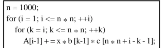
Fig. 7. The program segment of Adjoint Convolution. n = 1000;
for (i = 1; i <= n * n; ++i) for (k = i; k <= n * n; ++k)
A[i-1] + = x * b [k-1] * c [n * n + i - k - 1];
∑ Phase 1: The following attributes can be obtained from the input file.
1. The loop is the 4th type (AC). 2. The program size is large.
3. The loop has decreasing workload, which means it is the 3rd style. 4. There is slight affinity in this example, that means no.
5. The loop bound is known during compiler time. 6. The loop is nested.
7. Loop carried dependence distance is zero, that means DOALL.
∑ Phase 2: Post to inference, IPLS finds that the constraints of TSS are satisfied and
deter-mines that TSS is the most suitable algorithm.
∑ Phase 3: The TSS is invoked to transform the loop into a multithread program as shown
as Fig. 8. The TSS algorithm partitions and schedules the iterations of Adjoint Convolution.
∑ Phase 4: While the loop is being executed, the profile information is generated and
4. EXPERIMENTAL RESULTS
In this section, two parts of an experiment will be examined for IPLS. The first part of the experiment is based on a UMA system. The other is simulation of a NUMA system by using a UMA system.
4.1 Experimental Environment
Our target machine was a two Pentium-133 CPU multiprocessor system, running the Windows NT multithreaded OS that supports Win32 API functions. The system included a 512K external cache, 64MB shared-memory, and a 64-bit high-speed frame bus. Our pro-gramming tool was visual C++, which provides Win32 API function call. Due to the symmet-ric architecture, computation tasks could be easily distributed to any available processor.
4.2 Applications
Ten popular application programs were chosen and executed in UMA and NUMA environments. These applications were discussed in section 3 and represent different loop types. We tested these applications as follows to show the feasibility and generalization of IPLS.
1. Adjoint Convolution: The loop in this application has a decreasing workload; only the outer loop can be parallelized and the ith iteration takes O(N2- i) time. It has no data affinity to exploit.
2. Reverse Adjoint Convolution: This program has an increasing workload. As the loop bound i increases from 1 to N2, the workload also increases from O(1) to O(N2). 3. Gaussian Elimination: This program has a small load imbalance across iterations and has
some data affinity between matrix references. The inner loop can be parallelized. 4. Matrix Multiplication: This, the most commonly used program in parallel processing,
has a uniform workload. Since Matrix A rows and Matrix B columns are referenced constantly, and the elements of both Matrices are not modified, and a local cache, if available, will be very useful to the system.
5. All Pairs Shortest Paths: The workload of the ith iteration of the inner parallel loop
depends on A[i][k], and it takes O(1) or O(N) times to complete the work. Because each processor’s work queue initially contains about N/P consecutive iterations, the total loads for all the processors are about the same. Load imbalance is not significant. The
ith iteration always accesses the ith row of the matrix. Therefore, the application has to
exploit the affinity effect.
6. Successive Over-Relaxation (SOR): All the iterations of the SOR parallel loop take about the same time to execute, and each iteration always accesses the same set of data. Exploiting processor affinity may improve performance better than balancing the workload can. In this application, each parallel iteration has a locality rate of one and a data set of N array elements. The computational granularity of each parallel iteration is O(N). 7. Jacobi Iteration: In the JI program, the top 20% of the rows of elements in the non-singular
matrix A are nonzero elements, which are generated by a random number generator. The iterations of the parallel loop have a different workload, which is determined by the distribution of nonzero elements in A, so exploiting load imbalance will improve the performance. However, the workload of each parallel iteration is not changed when it is executed repeatedly.
8. LU Decomposition: This consists of an outer sequential loop and a parallel loop. In the innermost loop, one of the rows of the matrix A is modified based on the pivot row k. 9. Gauss-Jordan Elimination: The iteration granularity of Gauss-Jordan Elimination is small
and is independent of the program size. The amount of variance in the iteration length is small, too. Programs of this kind are more suitable for static scheduling schemes than scheduling schemes. To outperform the static scheduling scheme problems, self-scheduling schemes must be able to achieve load balance with very small self-scheduling overhead.
10. Transitive Closure: The characteristic of this program is that the workload depends on the input data. Each iteration takes either O(1) or O(N) time. Since the input data af-fects the amount of execution time, the workload is randomly.
4.3 Experimental Results on a UMA System
Because the restriction of the operating system to programmers, a system function call for binding any thread onto a specific processor is not available and only dynamic scheduling is allowed to use on this experiment. There were two kinds of experiments on a UMA system and a NUMA system. One studied the execution time and speedup of above ten applications, and the other examined a combined case that included ten applications in a program.
4.3.1 The implementation on the UMA system
Let us examine the implementation on the UMA system, which was a 2-processor machine; the execution time and the corresponding speedup are shown in Table 7 and Fig. 9, respectively.
Table 7. The execution time (ms)/speedup of 11 applications obtained by applying different scheduling algorithms.
Applications SERIAL CSS/2 GSS TSS Factoring SSS AHS IPLS Adj-Con 20104/1 15042/1.337 15055/1.335 10398/1.933 13974/1.439 12359/1.627 12352/1.628 as TSS Gauss_Eli 365359/1 256945/1.422 197157/1.853 202922/1.8 195016/1.873 208055/1.756 196852/1.856 as Factoring Gauss_Jor 7765/1 4245/1.829 5587/1.39 5599/1.387 5266/1.475 4333/1.792 4391/1.768 as CSS/2 Jacobi_Iter 14047/1 10109/1.39 12836/1.094 12656/1.11 13125/1.07 9802/1.433 9758/1.44 as AHS LU 40995/1 28094/1.459 33521/1.223 34356/1.193 33071/1.24 28505/1.438 28432/1.442 as CSS/2 Matrix_Mul 23453/1 12281/1.91 12095/1.939 12229/1.918 12214/1.92 12187/1.924 12203/1.922 as CSS/2 Radj_Con 27235/1 21274/1.28 14719/1.85 15587/1.747 15255/1.785 14336/1.9 15477/1.76 as SSS Saor 109062/1 76891/1.418 82594/1.32 83943/1.299 86742/1.257 38126/1.41 77680/1.404 as CSS/2 Spath 63063/1 57032/1.106 58867/1.071 43146/1.462 310469/1.543 295922/1.619 296078/1.618 as SSS Tran_Clos 479188/1 298312/1.606 308844/1.552 325430/1.472 310469/1.543 295922/1.619 296078/1.618 as SSS If_Then 17125/1 9682/1.769 9693/1.767 8595/1.992 8667/1.976 8656/1.978 8620/1.987 as AHS
GSS performed poorly for Adjoint Convolution because the workload of the iterations is decreasing and TSS is the most efficient algorithm for Adjoint Convolution (shown in Fig. 5.1(a)). CSS/2 was suitable for the applications like Gauss Jordan Elimination with a random unbalanced workload, LU Decomposition with a decreasing imbalanced workload, and SOR with a uniform balanced workload (shown in Fig. 5.1(c), (e), (h)) respectively. The factoring scheduling algorithm wass suitable for Gauss Elimination with a random balanced workload (shown in Fig. 5.1 (b)). SSS was suitable for applications like Reverse Adjoint Convolution with an increasing imbalanced workload, All Pairs Shortest Paths with a random balanced workload, and Transitive Closure with a random unbalanced workload (shown in Fig. 5.1(g), (i), (j)), respectively. AHS was suitable for Jacobi Iteration with a random unbalanced workload (shown in Fig. 5.1(d)). We can find that none of six scheduling algorithms under UMA system was suitable for all applications. IPLS could choose an appropriate scheduling algorithm and get good performance for most of the applications except Matrix Multiplica-tion and If_Then. In the case of Matrix MultiplicaMultiplica-tion, IPLS did not apply the optimal approach, GSS, but chose CSS/2 because the workload of iterations in this program is uniform. However, the number of processors, 2, was so small that CSS could not exploit the ability fully. In the case of the If_Then application, IPLS did not apply the optimal approach, TSS, but chose AHS because AHS is suitable for a random workload of iterations in the program. The reason for not selecting an optimal approach was similar to that for the case of Matrix Multiplication. Although the selection of scheduling algorithms was not absolutely accurate, we could solve the problem by refining the attributes causing the error. The refining system in IPLS will be used afterwards. Traditionally, once a scheduling algorithm is used, it will be used through out the entire program. But IPLS can always choose an appropriate schedul-ing algorithm accordschedul-ing to the behaviors of the loops among one program. A comparison of results obtained using KPLS and IPLS on a UMA system is shown in Table 8.
In the second experiment, IPLS chose different scheduling algorithms for each loop in the combined program integrated from the above eleven applications. For example, accord-ing to the loop behaviors, IPLS selected TSS for the Adjoint Convolution part of the com-bined program and chose factoring for the Gauss Elimination part, instead of choosing only one scheduling method. Table 9 and Fig. 10 show, respectively, the experimental execution time and the corresponding speedup for the combined program.
4.3.2 The simulation results on the UMA system
To overcome the problem of the limit of only 2 processors in the UMA system in our experiment, we simulated multiprocessor systems with 4, 8, 16 and 32 processors on our target machine with 2 processors, and the results are shown in Table 10.
From the simulation on the UMA system, some significant results were obtained: On the UMA system, generally speaking, the greater the number of processors, the better the performance of the applications with DOALL loops while applying each scheduling algorithm, and the number of processors also influenced the selection of loop scheduling algorithms.
Fig. 10. The speedup of the combined program for different kinds of loop scheduling. Table 9. The execution time (ms)/speedup of the combined program for different
scheduling algorithms.
Applications Serial CSS/2 GSS TSS Factoring SSS AHS IPLS All 1167396/1 789907/1.477 750968/1.554 754511/1.547 755346/1.545 709657/1.645 700640/1.666 693687/1.683
Table 8. A comparisons of results obtained by applying KPLS and IPLS.
Applications Best Loop Scheduling KPLS Result IPLS Result
Adj_Con TSS as TSS as TSS
Gauss_Eli Factoring as Factoring as Factoring
Gauss_Jor CSS/2 as CSS/2 as CSS/2
Jacobi_Iter AHS as TSS as AHS
LU CSS/2 as CSS/2 as CSS/2 Matrix_Mul GSS as CSS/2 as CSS/2 Radj_Con SSS as Factoring as SSS SOR CSS/2 as CSS/2 as CSS/2 Spath SSS as TSS as SSS Tran_Clos SSS as TSS as SSS
Table 10. The execution time (ms) of 11 applications for different scheduling algorithms on the UMA system with 4, 8, 16 and 32 processors.
Adjoint Convolution
Processor number Serial CSS GSS TSS Factoring SSS A H S IPLS
4 2 0 1 0 4 8 6 3 7 8 6 8 4 4 9 4 4 4 9 4 2 6 7 7 3 6 9 2 1 as TSS 8 2 0 1 0 4 4 6 2 8 4 6 6 2 2 4 9 3 2 4 7 1 3 5 5 1 3 6 3 7 as TSS 1 6 2 0 1 0 4 2 3 9 3 2 3 9 2 1 2 5 6 1 2 3 7 1 8 0 9 1 8 4 4 as TSS 3 2 2 0 1 0 4 1 2 1 8 1 2 1 6 6 5 2 6 2 1 9 1 6 9 3 9 as TSS
Gauss Elimination
Processor number Serial CSS GSS TSS Factoring SSS A H S IPLS
4 3 6 5 3 5 9 1 3 4 6 8 5 9 5 0 5 2 9 0 7 6 4 4 9 5 9 1 0 1 0 3 4 3 0 1 0 3 5 3 9 as GSS 8 3 6 5 3 5 9 6 8 6 1 9 5 0 1 7 8 5 5 8 1 9 5 1 1 7 9 5 4 1 7 1 5 4 0 8 9 as GSS 1 6 3 6 5 3 5 9 3 5 0 7 5 2 7 4 1 8 3 0 7 9 6 2 8 3 6 8 2 8 9 6 6 2 8 9 7 4 as GSS 3 2 3 6 5 3 5 9 1 8 7 7 1 1 6 8 5 3 1 7 5 2 1 1 7 4 8 3 1 6 8 4 3 1 6 8 5 9 as GSS
Gauss-Jordan Elimination
Processor number Serial CSS GSS TSS Factoring SSS A H S IPLS
4 7 7 6 5 2 1 5 3 2 6 9 2 2 4 5 3 2 4 5 6 2 6 1 8 2 6 1 8 as CSS 8 7 7 6 5 1 2 0 7 1 7 0 2 1 4 6 0 1 4 6 2 1 6 1 5 1 5 9 0 as CSS 1 6 7 7 6 5 7 3 2 1 1 5 9 9 4 1 9 5 6 1 0 7 6 1 0 6 1 as CSS
3 2 7 7 6 5 5 0 1 8 6 2 7 0 5 7 1 6 7 7 7 7 7 5 as CSS
Jacobi Iteration
Processor number Serial CSS GSS TSS Factoring SSS A H S IPLS
4 1 4 0 4 7 3 5 9 9 4 2 1 6 4 2 9 3 4 5 1 8 5 0 9 4 4 2 4 6 as CSS 8 1 4 0 4 7 1 9 9 6 2 4 6 8 2 3 5 2 2 6 9 2 2 8 9 5 2 4 9 0 as CSS 1 6 1 4 0 4 7 1 0 6 8 1 5 8 1 1 4 3 8 1 6 7 6 1 7 7 3 1 6 5 0 as CSS 3 2 1 4 0 4 7 6 3 1 1 0 2 6 1 0 5 8 1 1 2 3 1 0 6 0 1 0 6 5 as CSS
LU Decomposition
Processor number Serial CSS GSS TSS Factoring SSS A H S IPLS
4 4 0 9 9 5 1 0 4 7 5 1 1 5 0 1 1 1 7 1 7 1 1 9 7 8 1 1 2 2 7 1 1 2 9 6 as CSS 8 4 0 9 9 5 5 7 7 1 6 4 7 0 6 1 4 8 6 7 4 8 6 3 5 5 6 3 4 4 as CSS 1 6 4 0 9 9 5 3 3 5 7 3 7 9 8 4 1 6 5 3 8 9 1 3 4 7 3 3 4 7 0 as CSS 3 2 3 0 9 9 5 2 1 7 2 2 3 7 3 2 4 0 8 2 2 3 6 2 3 3 6 2 3 3 1 as CSS
Matrix Multiplication
Processor number Serial CSS GSS TSS Factoring SSS A H S IPLS
4 2 3 4 5 3 5 9 0 9 5 9 5 5 5 8 4 6 5 9 4 3 5 9 4 6 5 8 4 1 as CSS 8 2 3 4 5 3 2 9 7 5 3 0 2 5 3 1 1 8 2 9 9 4 3 1 6 8 3 1 1 1 as CSS 1 6 2 3 4 5 3 1 4 8 9 1 6 3 8 2 1 0 7 1 5 1 2 1 7 7 8 1 7 6 2 as CSS 3 2 2 3 4 5 3 7 5 5 8 5 9 7 8 2 7 5 9 9 2 0 9 0 3 as CSS
Reverse Adjoint Convolution
Processor number Serial CSS GSS TSS Factoring SSS A H S IPLS
4 2 7 2 3 5 1 1 9 3 4 6 9 3 7 6 8 3 2 6 8 2 0 7 1 1 0 7 1 3 4 as GSS 8 2 7 2 3 5 6 3 6 0 3 4 5 1 3 5 4 2 3 4 1 2 3 5 8 5 3 2 6 4 as GSS 1 6 2 7 2 3 5 3 3 8 1 1 7 4 1 1 8 7 7 1 7 8 1 1 8 5 9 1 8 8 4 as GSS 3 2 2 7 2 3 5 1 6 9 5 8 7 9 9 4 6 8 9 9 9 4 5 9 5 9 as GSS
SOR
Processor number Serial CSS GSS TSS Factoring SSS A H S IPLS
4 1 0 9 0 6 2 2 1 8 0 5 2 9 2 0 4 2 9 5 7 2 3 0 1 0 8 2 9 1 2 4 2 9 1 6 6 as CSS 8 1 0 9 0 6 2 1 4 5 3 8 5 6 1 6 1 5 6 3 4 1 6 1 6 9 1 5 5 4 5 1 5 5 7 2 as CSS 1 6 1 0 9 0 6 2 7 9 3 9 8 5 6 5 9 7 9 7 8 8 2 2 8 9 1 5 8 8 6 5 as CSS 3 2 1 0 9 0 6 2 4 2 2 1 4 6 9 3 4 6 6 8 4 7 1 3 5 2 6 1 5 2 9 7 as CSS
All Pairs Shortest Paths
Processor number Serial CSS GSS TSS Factoring SSS A H S IPLS
4 6 3 0 6 3 1 6 0 9 5 1 7 0 5 2 1 7 2 2 3 1 7 5 9 1 1 6 8 9 8 1 7 1 0 0 as CSS 8 6 3 0 6 3 8 2 9 2 9 5 3 9 8 7 5 9 9 8 3 5 9 5 0 7 9 3 6 5 as CSS 1 6 6 3 0 6 3 4 4 6 8 5 5 6 0 5 8 0 2 5 7 2 5 5 4 5 5 5 4 5 2 as CSS 3 2 6 3 0 6 3 2 7 9 0 3 7 0 8 3 6 9 8 3 1 5 9 3 7 2 3 3 7 1 1 as CSS
Transitive Closure
Processor number Serial CSS GSS TSS Factoring SSS A H S IPLS
4 4 7 9 1 8 8 1 2 6 2 5 8 1 2 2 5 8 1 1 2 6 5 2 7 1 2 4 9 7 1 1 2 3 3 0 2 1 2 2 9 9 9 as SSS 8 4 7 9 1 8 8 6 4 4 1 2 6 4 4 2 3 6 4 3 1 8 6 5 0 8 8 6 3 3 3 6 6 3 7 2 4 as SSS 1 6 4 7 9 1 8 8 3 3 4 7 0 3 4 5 0 9 3 4 1 2 1 3 5 5 8 8 3 4 3 3 1 3 4 9 0 3 as SSS 3 2 4 7 9 1 8 8 1 8 2 0 6 1 9 6 1 1 2 2 3 5 8 1 9 9 6 0 1 8 9 7 4 1 9 0 2 6 as SSS