Optimizing the packet forwarding throughput of multi-hop wireless chain networks

Optimizing the packet forwarding throughput of multi-hop

wireless chain networks

S.Y. Wang*

Department of Computer Science and Information Engineering, National Chiao Tung University, 1001, Ta-Hseuh Road, Hsinchu 30050, Taiwan, ROC Received 19 April 2002; revised 1 January 2003; accepted 20 January 2003

Abstract

In the literature, it has been shown that due to signal interferences between neighboring stations, the maximum packet forwarding throughput of a N-hop wireless chain network decreases as N increases and is only 1=N of the wireless bandwidth. This 1=N trend continues until the throughput finally stabilizes at only 1/5 or even less when N becomes large. To solve this problem, this paper proposes an approach that optimizes the forwarding throughput of a wireless chain network. In this approach, which we call the ‘two-frequency scheme’, the wireless interface cards of some nodes in the wireless chain network will swap their operating frequency channels between two different channels to avoid interferences. Using this approach, even when N is large, the forwarding throughput can be cost-effectively improved to 1/2, which is the optimal forwarding throughput that can be achieved by a half-duplex wireless interface.

q2003 Elsevier Science B.V. All rights reserved.

Keywords: Wireless network; Medium access control; Ad hoc network

1. Introduction

In this paper, we study the maximum forwarding throughput of a chain of wireless stations (called ‘a wireless chain network’ in this paper). The stations of a wireless chain network can be either mobile or fixed and they are located roughly on a line (need not be absolutely straight) as depicted in Fig. 1. The primary usage of a wireless chain network is that it can be used as a forwarding (relaying) path to extend the coverage range of a wireless network. In real life, because the coverage range of a single-station wireless network is limited (e.g. the coverage range of an IEEE 802.11[1]wireless station is only several hundred meters), using a wireless chain network to relay packets is therefore desired.

To maximize the extension of a wireless chain network, normally wireless stations are placed in a way such that the coverage range of a wireless station covers only its two neighboring stations. As shown in Fig. 1, the coverage range of wireless station ðiÞ covers only wireless station ði 2 1Þ and station ði þ 1Þ; but not station ði 2 2Þ and station ði þ 2Þ:

The wireless chain network is widely used in wireless relay networks which connect two distant sites together. The wireless chain network also exists in a multi-hop wireless network, regardless of the multi-hop wireless network’s topology. On a multi-hop wireless network, because a unicast routing path is composed of a chain of wireless stations, a unicast routing path that is actively used to forward packets can be viewed as a wireless chain network by itself. Maximizing the packet forwarding throughput of a chain of wireless stations therefore is important not only to a wireless chain network, but also important to mobile ad hoc networks. In practice, a wireless station normally uses only one wireless network interface card (NIC) to send, receive, and forward packets. (Each wireless NIC normally uses only one radio.) In this case, it is easy to derive the maximum forwarding throughput of a N-hop ðN ¼ 1; 2; and 3Þ wire-less chain network. When N is 1, the maximum forwarding throughput can be 1 (i.e. 100% of the wireless bandwidth) because the sending station can keep transmitting packets to the receiving station. (Note: to save space, in the following, we will simply use a number to represent the fraction of the wireless interface’s bandwidth.) When N is 2, the maximum forwarding throughput is only 1/2 because of the half-duplex property of the middle (forwarding) station’s wireless NIC. When N is 3, the maximum forwarding 0140-3664/03/$ - see front matter q 2003 Elsevier Science B.V. All rights reserved.

doi:10.1016/S0140-3664(03)00035-5

www.elsevier.com/locate/comcom

* Corresponding author. Tel.: þ886-3-5131550; fax: þ886-3-5724176. E-mail address: [email protected] (S.Y. Wang).

throughput is only 1/3. The reason is that, to avoid collisions, at any time, packet transmission can occur on at most one hop among these three hops. For example, inFig. 1, when station ði 2 2Þ forwards a packet to station ði 2 1Þ; station ðiÞ cannot forward a packet to station ði þ 1Þ at the same time. Otherwise, the signal of the packet sent from station ðiÞ to station ði þ 1Þ will reach station ði 2 1Þ and collide with the packet sent from station ði 2 2Þ to station ði 2 1Þ:

When N further increases, simulation and experimental results both show that the achieved forwarding throughput further decreases and finally stabilizes at about 1/5 [2] or even less (1/7)[3]. These results also show that the transport protocol (e.g. TCP or UDP) used by the packets being forwarded actually is irrelevant to this low forwarding throughput problem.

Because 1/5 (or 1/7) is low compared to 1/2 (the maximum forwarding throughput of a wireless NIC) and a chain of wireless stations is a common topology, this low forwarding throughput problem is important and motivated our work. Our approach, which we call the ‘two-frequency scheme’ in this paper, is based on IEEE 802.11 MAC protocol. It is a slight modification of the 802.11 protocol with a signaling protocol used to configure the stations of a wireless chain network. In this approach, the wireless NICs of some nodes in the wireless chain network will swap their operating frequency channels between two different chan-nels to avoid interferences.

The contribution of this paper is that we propose a cost-effective approach that optimizes the forwarding throughput of a multi-hop wireless chain network. Allowing each wireless station to still use only one wireless NIC (i.e. one radio), our approach cost-effectively improves the forward-ing throughput from 1/5 (or 1/7) to 1/2, which is a 250% (or 350%) improvement.

The design of the two-frequency scheme focuses on improving the packet forwarding performance of a wireless chain network. Spectrum efficiency is not the focus of this paper. However, even from a performance/spectrum efficiency viewpoint, the two-frequency scheme is still more efficient than simply using twice spectrum (i.e. the spectrum used by two frequency channels) to double a wireless NIC’s transmission capability. This is clear as (1/2)/2 is still greater than (1/5)/1 (or (1/7)/1).

The rest of this paper is organized as follows: Section 2 surveys related work. Section 3 describes the wireless NIC parameters used in the paper. Section 4 presents the design and implementation of the two-frequency scheme. Section 5

presents simulation results showing the performances of the two-frequency scheme under various conditions. Section 6 discusses the applications of the two-frequency scheme to lattice and mobile ad hoc networks. Finally, Section 7 concludes the paper.

2. Related work

In the literature, the authors in Refs. [4 – 6] used the GloMoSim [7] simulator to compare the effects of several MAC protocols on TCP’s performance over multi-hop wireless networks. Using a CSMA/CA MAC protocol, which is similar to IEEE 802.11 MAC protocol, they found that when the maximum window size of a greedy TCP connection is set to only one packet, the TCP connection could achieve a better throughput. However, when the maximum window size is set to multiple packets, the TCP connection’s achieved throughput instead decreases sub-stantially. They explained this phenomenon with the following reasons: (1) If the TCP maximum window size is greater than one packet, more than one TCP data packets will traverse on multiple wireless hops. (2) These TCP data packets will contend with returning TCP ACK packets for wireless bandwidth on multiple wireless hops. (3) These contentions may cause packet collisions and thus result in poor TCP throughput.

When the TCP maximum window size is set to only one packet, they further found that the throughput of a greedy TCP connection over a N-hop wireless chain network decreases as N increases. It was also observed that the achieved throughput roughly is 1=N until it finally stabilizes at around 1/5 when N is 5. The authors attributed this 1=N trend to the use of the 1-packet TCP maximum window size over a N-hop wireless chain network and the contention of TCP’s two way traffic on multiple wireless hops.

In Ref. [2], the authors did a similar simulation study. The simulator used was the ns network simulator [8]with the CMU Monarch project’s IEEE 802.11 wireless module. The authors used the simulator to obtain the throughput of a greedy TCP connection over a N-hop wireless chain network. The authors also found the 1=N trend but did not investigate the causes of it. Instead, they just used the simulation results to derive a TCP connection’s expected throughput on a mobile ad hoc network. Since their focus was not on understanding the causes nor on improving the achieved throughput, they referred readers to the papers listed in Refs.[4 – 6]and did not give explanations.

Fig. 2shows a copy of a figure presented in Ref.[2]. This figure shows the achieved throughput of a greedy TCP connection over a N-hop wireless chain network. Although the authors used a different network simulator (ns) than the one (GloMoSim) used in the papers [4 – 6], the 1=N trend still clearly exists. The authors did not report the TCP maximum window size that they used in their simulations. They did not report that setting the TCP maximum window Fig. 1. A chain of wireless stations used as a forwarding path.

size to one packet could improve the throughput of a TCP connection.

In Ref. [3], the authors used their simulation and experimental results to explain the 1=N trend. When N # 4; they attributed the 1=N trend to signal interferences between neighboring stations. When N . 4; they attributed the 1=N trend to uneven competitions experienced by the stations on a wireless chain network. Their simulation and experimental results show that the maximum forwarding throughput that a wireless chain network can provide for a greedy flow is only 1/7 when the number of hops is large.

To summarize, although these related papers observed or explained the 1=N trend, none of them provided a solution to this 1=N low forwarding throughput problem. Our paper is the first paper that provides a solution to this problem.

3. Wireless NIC parameters

We used the NCTUns 1.0 network simulator [9] to perform simulation studies. The NCTUns 1.0 is a high-fidelity and extensible network simulator just released to the networking community and is available for download at

http://NSL.csie.nctu.edu.tw/nctuns.html. We ported the CMU Monarch project’s IEEE 802.11 wireless module from ns to the simulator. Therefore, the IEEE 802.11 MAC-layer parameters used in the simulator are the same as those used in ns. To reflect the fact that 802.11 2 Mbps products have been replaced by 802.11 (b) 11 Mbps products in the current markets, the bandwidth of wireless interfaces in the simulator is changed from 2 to 11 Mbps. This physical-layer change does not affect the 1=N trend.

Note that the maximum throughput that can be achieved on a single-hop 802.11 (b) 11 Mbps network is only about 7 Mbps. This is due to the 802.11 MAC protocol design in which (1) the inter-frame gap time is fixed in both the 2 Mbps and 11 Mbps versions, and (2) the physical-layer header of every 802.11 MAC frame is transmitted at 1 Mbps for backward compatability issues. As a result, when the wireless bandwidth is increased from 2 to 11 Mbps, the efficiency of the wireless medium (air) usage decreases. Ns also generates the same maximum throughput when we

change its wireless bandwidth from 2 to 11 Mbps. Besides, the Lucent Orinoco 11 Mbps IEEE 802.11 (b) wireless NIC generates the same maximum throughput as well. We point out this phenomenon because we want to make the definition of 1=N clear. When we say 1=N in the rest of the paper, actually we mean (1/N £ the maximum throughput achievable on a single-hop IEEE 802.11 network). It is not (1/N £ the bandwidth of a wireless NIC).

In the CMU Monarch project’s wireless module, the radio propagation model used is the 2-ray ground reflection model [10], the receive (RX) power threshold used is 3:652 £ e210; and the carrier sense (CS) power threshold used is 1:559 £ e211: Under the 2-ray model, the distances between the sender and receiver that correspond to the RX and CS thresholds are 250 and 550 m, respectively. These two ranges are called ‘transmission range’ and ‘interference range’, respectively, in the rest of the paper. In our simulation study, the distance between neighboring stations on a wireless chain network is set to 240 m.

4. The two-frequency scheme

Because the two-frequency scheme is based on the IEEE 802.11 design, we will present some relevant background of IEEE 802.11 in Section 4.1. Readers who are familiar with IEEE 802.11 can skip Section 4.1 without loss of continuity. 4.1. IEEE 802.11 overview

The stations of a wireless chain network use the ad hoc mode to communicate with their neighboring stations. Therefore, we will briefly present the IEEE 802.11 Distributed Coordination Function (DCF) [1], which is a CSMA/CA MAC protocol used in the ad hoc mode.

DCF performs link-layer retransmission of data frames to reduce a frame’s effective Packet-Error-Rate (PER) on a wireless link. The receiving station needs to send a link-layer ACK frame to the sending station to indicate the success or failure of receiving a data frame. If an expected ACK frame is not received in a certain time, the sending station will retransmit the data frame until a maximum-retry limit is exceeded. (In 802.11, the maximum-retry limit is four for large frames and seven for small frames.) At that time, the current data frame is discarded, the retry count is reset to 0, and a new data frame is transmitted.

To avoid frame duplications, every sending station maintains a sequence number. The sequence number is increased by one when each new data frame is transmitted. When a data frame is transmitted, the current sequence number is copied into its header. The receiving station can detect duplicate frames by comparing the sequence number carried in the just received frame with a sequence number that was most recently received from the same sending station.

Fig. 3(a) depicts the DATA/ACK frame exchange sequences, where SIFS and DIFS are the inter-frame gap Fig. 2. The 1=N trend simulation results reported in Ref.[2].

times. (In 802.11 DSSS specification, SIFS and DIFS are 10 and 50 ms, respectively.)

To reduce collisions caused by hidden terminals in a wireless network, DCF provides an option in which four-way RTS/CTS/DATA/ACK frame exchange sequences are used. Before sending a data frame, the sending station first sends a RTS (request-to-send) frame to the receiving station. On receiving the RTS frame, the receiving station sends a CTS (clear-to-send) frame back to the sending station. After receiving the CTS frame, the sending station then sends a data frame to the receiving station. The receiving station then sends back an ACK frame to the sending station if it can successfully receive the data frame. The purpose of sending RTS and CTS frames is to announce to other neighboring stations that a frame transfer will soon occur and they should keep ‘quiet’ for some time to avoid collisions. Fig. 3(b) depicts the RTS/CTS/DATA/ACK frame exchange sequences.

To transmit a data frame, either the DATA/ACK or the RTS/CTS/DATA/ACK frame exchange sequence can be used. The decision can be controlled on a per-frame basis by comparing the data frame length with the value of the RTS threshold.

Currently, IEEE 802.11 (b) wireless NICs are popular in the market. These NICs can transmit at a maximum rate of 11 Mbps and use a channel out of 11 different channels under USA FCC regulation. (Note: under Europe ETSI regulation, there are 13 available channels to choose from.) More detailed information about IEEE 802.11 can be found in Ref.[1].

4.2. Design of the two-frequency scheme 4.2.1. Macroscopic behavior

We call our scheme the ‘two-frequency scheme’. This is because in the scheme, two frequency channels are used in

a wireless chain network. We note that although in the scheme two frequency channels are used, every wireless station needs to use only one wireless NIC.

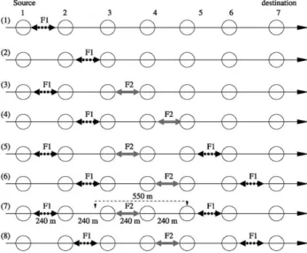
In the scheme, time is divided into fixed-length time slots. The length of these time slots is a system parameter of the scheme. In a time slot, a station is configured to exchange frames only with one (the left side or the right side) of its two neighboring stations. When the current time slot ends and the next time slot begin, the station will exchange frames only with its another neighboring station. That is, in consecutive time slots, station ðiÞ will swap it communication partner between station ði 2 1Þ and station ði þ 1Þ: For example,Fig. 4shows that station (2) swaps its communication partner between station (1) and station (3) in consecutive time slots. (Note: A pair of stations that are each other’s communication partner is represented by a thick line with two arrows here.) Because a station needs to change its communication partner in consecutive time slots and the head-of-line blocking problem should not occur, a station maintains two output queues for its wireless NIC—one for frames that need to be forwarded to its right communication partner and the other for frames that need to be forwarded to its left communication partner.

When a wireless chain network is brought up, each station’s initial communication partner for time slot (1) is properly configured by the use of a signaling protocol. This ensures that when the wireless chain network is operating, the following two communication patterns will alternate in consecutive time slots. In the first communication pattern, station ðj 2 1Þ and station ðjÞ are each other’s communi-cation partner, j ¼ 2; 4; 6; …; etc. In the second communi-cation pattern, station ðj 2 1Þ and station ðjÞ are each other’s communication partner, j ¼ 3; 5; 7; …; etc. For example,

Fig. 4shows that in time slot (6) the communication pattern is ((2, 3), (4, 5), (6, 7),…), in time slot (7) the pattern Fig. 3. The two different frame exchange sequences used in the IEEE

802.11 CSMA/CA MAC protocol: (a) DATA/ACK (b) RTS/CTS/DA-TA/ACK.

Fig. 4. The frequency channel and communication partner swapping schedule in the two-frequency scheme, where (1), (2), (3), (4), (5), (6), (7), and (8) are consecutive time slots. This figure shows how data frames are pipelined into the wireless chain network from left to right.

changes to ((1, 2), (3, 4), (5, 6),…), and in time slot (8) the pattern changes back to ((2, 3), (4, 5), (6, 7),…).

As a wireless chain network is swapping its communi-cation pattern between the two different patterns described above, data frames can be forwarded from one end to the other end of the wireless chain network. For example, a data frame which is originated on station (1) will be forwarded to station (2) in time slot ðiÞ; then from station (2) to station (3) in time slot ði þ 1Þ; then from station (3) to station (4) in time slot ði þ 2Þ; and so on. It is clear that if a wireless chain network has N hops and the time slot length is T ms, it would take a data frame ðN £ TÞ ms to traverse the whole wireless chain network. For this reason, the time slot length should be kept as small as possible while allowing the wireless chain network to have a high forwarding throughput. Since two neighboring stations can exchange their frames when they are each other’s communication partner, a wireless chain network in the scheme is bidirectional. Besides, since there is no limitation on the number of frames that may be transmitted by any of these two neighboring stations, the traffic pattern on a wireless chain network in this scheme need not be symmetric. Actually, the traffic pattern can be arbitrary and dynamic.

We useFig. 4to illustrate the two-frequency scheme’s frequency channel and communication partner swapping schedule. Initially in time slot (1), stations (1, 2), (5, 6), ð4 £ i þ 1; 4 £ i þ 2Þ; …; i ¼ 0; 1; 2; …; are configured to use F1 and stations (3, 4), (7, 8), ð4 £ i þ 3; 4 £ i þ 4Þ; …; i ¼ 0; 1; 2; …; are configured to use F2. This channel assignment can be more clearly seen in time slot (7), in which the channel assignment is the same as that used in time slot (1). Even-numbered stations (e.g. station (2), (4), (6), etc.) are configured to use their initially assigned channels in all time slots. Odd-numbered stations (e.g. station (1), (3), (5), etc.), however, are configured to swap their channels between F1 and F2 in consecutive time slots. Because the wireless chain network is configured such that the communication partner pattern ((1, 2), (3, 4), (5, 6),…) is used in odd-numbered time slots and the pattern ((2, 3), (4, 5), (6, 7),…) is used in even-numbered time slots, the frequency channel and communication partner pattern of the wireless chain network will alternate between the pattern used in time slot (7) and that used in time slot (8).

The design of the two-frequency scheme effectively avoids the signal interference problem, which causes the 1=N trend. By using two frequency channels F1 and F2 alternatively along a wireless chain network, a station no longer can interfere a station that is not its communication partner but is using the same frequency channel. This is because now they must be at least three hops away. For example, inFig. 4, we see that when station (2) is using F1 to transmit a frame to station (1), the nearest station that is not station (2)’s communication partner but using the same channel F1 is station (5), which is three hops away from station (2). Suppose that these stations are placed D meters apart, where ð550=3Þ , D , 250: Because the distance

between station (2) and station (5) is larger than the interference range (550 m), station (5) will not be able to interfere station (2)’s transmissions.

The design of the two-frequency scheme is also cost-effective. First, the scheme can effectively improve the forwarding throughput of a wireless chain network. From

Fig. 4, we see that when a wireless chain network alternates between the patterns used in time slots (7) and (8), because the signal interference problem no longer exists, the forwarding throughput of the wireless chain network can be increased to the optimum of 1/2. (The optimum is 1/2 because it is the highest forwarding throughput that can be achieved by a wireless chain network in which every station uses only one half-duplex wireless NIC.)

Second, the scheme is a low-cost solution. Every station in the scheme still uses only one wireless NIC. Although one half of stations need to swap their frequency channels in consecutive time slots, the operation of swapping a station’s frequency channel can be performed easily and quickly in today’s technology. In Ref.[11], it is stated that current DSP technology enables radios to switch from one channel to the other within 1 ms. According to section 14.6.12 of IEEE 802.11 standard (‘99’version), it takes 224 ms to change a station’s operating frequency channel from one channel to another for FHSS. A reasonable number for DSSS would be somewhere between 20 and 200 ms. Even if the channel switching time is 200 ms, it still accounts for a very small overhead when the used time slot length is longer than several milliseconds. For example, when the time slot length used is 10 ms, the overhead of the frequency channel switching time is only 2%.

4.2.2. Microscopic behavior

At the end of a time slot, all stations will need to change their communication partners. Besides, some stations will also need to swap their channels. On every station, a timer is used and scheduled to periodically issue commands to trigger these operations.

Processing a command that requests a station to change its communication partner can be easily done. This is because the command just tells a station that when the current frame transmission is finished, the next frame to be transmitted should be dequeued from the other output queue and should no longer be dequeued from the current one. On the other hand, processing a command that requests a station to change its frequency channel should be done carefully. Otherwise, frame transmissions may fail unnecessarily, which will waste network bandwidth. For example, if a receiving station suddenly swaps its channel while it is receiving a frame, the received frame will be broken and the network bandwidth used for transmitting the frame will be wasted.

Fig. 5shows the eight different cases which a station may be in when it is time (represented by a dashed horizontal line) for the station to swap its channel. The meanings of these cases are explained below. We will use ‘the local station’ to mean the station that transmits data frames and

‘the remote station’ to mean the station that transmits back ACK frames.

Case 1

The frequency channel swapping command is issued after a DATA/ACK sequence is completed and before the local station starts the next DATA/ACK sequence.

Case 2

The command is issued when the local station is transmit-ting a data frame and the receiving station has started receiving the frame.

Case 3

The command is issued in the middle of a DATA/ACK sequence. That is, the data frame has been completely received by the remote station but the remote station has not started transmitting back the ACK frame.

Case 4

The command is issued when the remote station is transmitting back an ACK frame and the local station has started receiving it.

Case 5

The command is issued when the local station is transmit-ting a data frame but the frame has not arrived at the remote station yet.

Case 6

The command is issued when the remote station is transmitting back an ACK frame but the ACK frame has not arrived at the local station yet.

Case 7

The command is issued when the local station has finished transmitting a data frame but the remote station is still receiving the frame.

Case 8

The command is issued when the remote station has finished transmitting back an ACK frame but the local station is still receiving the ACK frame.

Among these cases, case 2 will occur much more frequently than the other cases. The time window in which

case 1 and 3 may occur is 50 (DIFS) and 10 (SIFS) ms, respectively. Because the transmission time of a 68 byte MAC-layer ACK frame on a 11 Mbps channel is 74 ms (74 ¼ 24 þ 50. 24 ms is the 802.11 physical-layer header’s transmission time and 50 ms is the MAC-layer ACK frame’s transmission time), the time window in which case 4 may occur is 74 ms. Cases 5, 6, 7, and 8 are caused by signal propagation delays in the air. Because the trans-mission range of 802.11 (b) stations are less than 1000 m, the signal propagation delay between two neighboring stations are only about 3 ms. As a result, the time windows for these cases are only about 3 ms. In contrast, in case 2, the transmission time of a 1500 byte data frame on a 11 Mbps channel is about 1000 ms. Because case 2’s time window is much larger than those for the other cases, case 2 will occur much more frequently than all other cases.

Below we will present the microscopic design of the two-frequency scheme. The designs and properties of the scheme are listed below:

† First, when a frequency channel swapping command is issued, the scheme will not abort or corrupt any ongoing frame transmission due to channel swapping. The local and remote stations will swap their channels only when the current transmission is finished and their wireless NICs become idle. This property enables the design to achieve a high forwarding throughput even when the time slot length is small. Without this design, as the time slot length decreases, because now more frames will be corrupted during channel swappings, the forwarding throughput will decrease.

† Second, when a command is issued, the local and remote stations will swap their channels right after the current transmission is finished, even though a complete DATA/ACK sequence may not have finished yet. That is, when the current data frame transmission is finished, the remote station will not intend to send back an ACK frame. Besides, the local station will not expect to receive an ACK frame because it knows that the remote Fig. 5. The eight different cases which a station may be in when it is time to for the station to swap it channel.

station will not send back an ACK frame in this design. Both stations will swap their channels immediately when the current transmission is finished. This property enables multiple stations’ channel and communication partner swapping operations to be finished quickly and almost at the same time. This is crucial to achieving a high forwarding throughput in the two-frequency scheme. (A pair of communication stations cannot fully utilize a time slot if they cannot swap their channels to the same channel quickly at the beginning of a time slot.) † Third, when a command is issued, the scheme does not use any control frame to perform any handshaking between the local and remote stations. This property enables the design to maintain a high forwarding throughput even when the time slot length is small. (Note: If in the design exchanging handshaking control frames were used during channel swappings, because exchanging handshaking control frames wastes network bandwidth and time, the forwarding throughput will decrease as the time slot length decreases.)

With these common properties, there are two different operating modes in the design. We call the first mode ‘the optimistic mode’ and the second mode ‘the pessimistic mode.’ Both modes have their own characteristics and strengths in different application areas. In the following, we will present both of them.

Optimistic mode. In the optimistic mode, the local station is optimistic about data frame transmissions. After transmit-ting a data frame, if it cannot receive an ACK frame due to a channel swapping, it always assumes that the remote station has successfully received the data frame. (Note that the data frame may actually be lost and the remote station may thus fail to receive it). Therefore, if the frequency channel swapping command is issued during a data frame trans-mission (as in case 2) or before the expected ACK frame comes back (as in case 3), the local station will view the transmission of the current data frame successful and remove it from the current output queue. A channel swapping operation will then take place as soon as the local station’s wireless NIC becomes idle. In this mode, if the last frame transmitted in a time slot is a new data frame (not a retransmission), it has the ‘at most once’ semantic.

Pessimistic mode. In the pessimistic mode, the local station is pessimistic about data frame transmissions. After transmitting a data frame, if it cannot receive an ACK frame due to a channel swapping, it always assumes that the remote station did not successfully receive the data frame. In this case, the current data frame is saved. It will be retransmitted at the beginning of the next next-time slot. For example, if the frequency channel swapping command is issued during a data frame transmission (as in case 2) or before the expected ACK frame comes back (as in case 3), the transmission of the data frame will be viewed as a failure

and be retransmitted later. In this mode, the last frame transmitted in a time slot has the ‘at least once’ semantic.

These two modes differ primarily in how they process case 2 and case 3. As for case 1 and case 4, respectively, the processing is the same in both modes. Case 1 is the simplest case to handle. Since the local and remote stations now are in the ready state, they can immediately swap their channels when the command is issued. In case 4, the ACK frame transmission is ongoing when the command is issued. The local station will wait until the entire ACK frame has been received. At that time, because a complete DATA/ACK sequence has finished, the local and remote stations can now swap their channels safely.

As for case 5, 6, 7, and 8, these cases are caused by signal propagation delays in the air. In case 5 and 6, a frame may be lost during channel swappings. The reason is that when the command is issued, the remote station has not received any data of the transmitted frame. It thus may decide to swap its channel to a different one, causing the frame to be lost when it arrives at the remote station. Although frames may be lost in case 5 and 6, these cases occur rarely due to their tiny time windows. Case 7 and 8 on the other hand will not cause a frame to be lost during channel swappings. After transmitting the last frame into the air, it is safe for the local or remote station to swap its channel.

4.2.3. Further improvement

To further improve the forwarding throughput, we studied the interactions between neighboring stations at the end of time slots. We found that sometimes after a station (say A) swaps its channel and communication partner, its new communication partner (say B) may not have finished swapping its channel to the one used by station A. As a result, when station A transmits a 1500 byte data frame to station B, this long frame is lost and the network bandwidth used for transmitting this long frame is totally wasted. Actually, in most cases, station B swaps its channel to the desired channel right after the first few bits of the data frame arrive. However, this partially received frame is already useless and the whole 1500 byte worth of bandwidth will be totally wasted.

To mitigate this problem, in the design we let the first data frame transmission in a time slot use the RTS/CTS/DA-TA/ACK sequence. RTS is a small frame (68 bytes only). It serves as an effective and efficient channel probing mechanism here. If the remote station has not swapped its channel to the channel that the local station is using, the local station’s sending a RTS frame to the remote station will not result in receiving a CTS frame from the remote station. Note that RTS’s transmission time is small and 802.11 (b) will retransmit RTS if no CTS is received in a certain period of time. For these reasons, when the remote station has swapped its channel to the desired one, the RTS/CTS mechanism can quickly detect this change without wasting too much bandwidth.

4.2.4. Comparison of the optimistic and pessimistic modes In Section 4.2.2, we pointed out that the optimistic mode has the ‘at most once’ semantic and the pessimistic mode has the ‘at least once’ semantic. Because these two semantics are different, a wireless chain network using the optimistic mode has different properties than the one that uses the pessimistic mode.

One difference is regarding the end-to-end PER of a wireless chain network. A wireless chain network that uses the pessimistic mode clearly will have a much smaller end-to-end PER than a wireless chain network that uses the optimistic mode, given a non-zero BER. This PER difference may be important or unimportant—depending on the application’s needs. For example, it may be unimportant for some type of traffic such as UDP. However, because a lost or corrupted TCP packet will trigger TCP congestion control, it is clear that TCP will perform poorly on a wireless chain that has a high PER.

Another difference is about packet duplication that a wireless chain network may impose on a packet stream. On a wireless chain network that uses the pessimistic mode, a frame may be unnecessarily retransmitted and thus be duplicated multiple times when it traverses the hops of a wireless chain network. Duplicate frames not only waste network bandwidth, they also unnecessarily trigger TCP congestion control when a TCP ACK packet is duplicated more than three times on it’s way to the TCP sender. (The famous TCP fast retransmit and rate reduction is triggered when more than three duplicate TCP ACK packets are received). It is clear that TCP will perform poorly if it is triggered by too many false alarms.

Although the two-frequency scheme uses the IEEE 802.11’s default duplicate frame detection mechanism. In the pessimistic mode, frame duplications may still happen. This is because the sequence number used by the last data frame in time slot ðiÞ and the sequence number that will be used to retransmit the same data frame at the beginning of time slot ði þ 2Þ may be different. This situation may occur because in time slot ði þ 1Þ some frames may have been transmitted to the other communication partner, and this will advance the sequence number maintained by the sending station.

Although both modes have their own strengths, because the simulation results show that TCP performance in the pessimistic mode is much worse than that in the optimistic mode (to be presented later inFig. 17), we suggest that the two-frequency scheme use the optimistic mode in most cases, unless the BER is excessively high. In the rest of the paper, we thus will focus on the performances of the optimistic mode.

5. Simulation results

In the following, we will present the performances of the two-frequency scheme that uses the optimistic mode.

5.1. Simulation settings

The traffic types used in the study are greedy UDP and TCP traffics. A greedy UDP flow is used as a traffic source because its offered load to a network is fixed and not sensitive to packet losses. In addition, its traffic is one-way traffic. As such, we used it to see how much forwarding throughput a wireless chain network can provide for a one-way and fixed-load greedy flow. We also used a greedy TCP flow as a traffic source because TCP’s offered load to a network is sensitive to packet losses. In addition, its traffic is two-way traffic. We used it to see how much forwarding throughput a wireless chain network can provide for a two-way and dynamic-load greedy flow, under various BERs. The maximum window size of a TCP connection is set to 245 KB. The version of TCP used is the version of TCP used in FreeBSD 4.4, which is based on TCP reno.

The system parameters that are varied in the simulations include: (1) the time slot length, (2) the number of hops of the wireless chain network, (3) the Bit-Error-Rate, (4) the type of the wireless chain network (using the normal 802.11 or the two-frequency scheme), and (5) the operating mode used in the two-frequency scheme.

The traffic configurations include: (1) single one-way UDP or TCP greedy flow, (2) two one-way UDP or TCP greedy flows competing in opposite directions. The performance metrics include: (1) the achieved throughput of a TCP or UDP flow, (2) the total forwarding throughput of a wireless chain network, (3) the end-to-end delay of a wireless chain network, and (4) the fairness in competing for the bandwidth of a wireless chain network.

In the following performance figures, each reported TCP or UDP throughput is an average of five runs each lasting 300 s of simulated time. Unless stated otherwise, BER is by default 0% and the default operating mode that a two-frequency wireless chain network uses is the optimistic mode.

5.2. Throughput issue

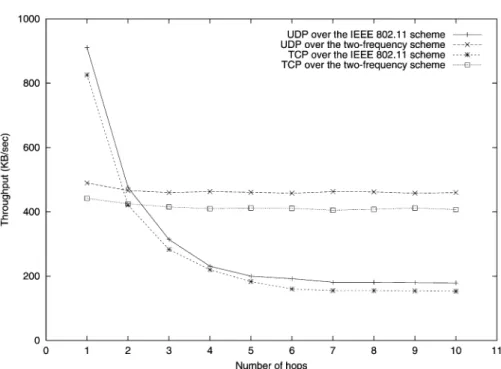
Two tests are performed to see how much forwarding throughput a wireless chain network can provide for greedy UDP and TCP traffic. In test 1, a greedy UDP flow is used as the traffic source. In test 2, instead, a greedy TCP flow is used. To save space, the results of test 1 and test 2 are plotted together inFig. 6. We can see that, for both UDP and TCP traffic, a two-frequency wireless chain network can provide a much higher forwarding throughput than an IEEE 802.11 wireless chain network.

The shape of the curves of the IEEE 802.11 scheme (for both UDP and TCP traffic) follows the curve depicted in

Fig. 6. (The reason has been explained in Section 1). We see that when the number of hop is 1, the IEEE 802.11 scheme can provide a higher throughput than the two-frequency scheme. The reason is that in this case the throughput is the transmission throughput directly between two nodes rather

than the forwarding throughput across several nodes. Because the two-frequency scheme is designed for for-warding packets across several nodes, it is inefficient in bandwidth for such a single-hop wireless chain network. Actually, since a single-hop wireless chain network does not have the signal interference problem presented in Section 1, there is no need to use the two-frequency scheme for it. 5.3. Fairness issue

To test whether a two-frequency wireless chain network can provide fair bandwidth sharings between greedy flows that compete in opposite directions on the network, we ran the following tests.

In test 1, two greedy UDP flows compete for the bandwidth of a two-frequency wireless chain network in opposite directions. In test 2, the competing greedy flows are replaced with TCP flows. To save space, the results of test 1 and test 2 are plotted together inFig. 7.

From the figure, we see that, either in the UDP or the TCP case, two greedy flows that compete in opposite directions can fairly share the bandwidth of the wireless chain network and the network bandwidth can be fully utilized.

We note that the design does not statically allocate 50% and 50% of the wireless chain network’s bandwidth to the forward and backward traffic. Instead, the fair sharing comes from the symmetric design of the two-frequency scheme. When two neighboring nodes become communi-cation partners in a time slot, they use the normal IEEE 802.11 (i.e. the MAC’s DCF) scheme to compete for the wireless bandwidth to send their packets to the other node.

As such, if both the forward and backward traffic loads are high, the two nodes (and thus the forward and backward traffic) will get about 50% and 50% of the wireless bandwidth.

5.4. Delay issue

In Section 4.2.1, we pointed out that if a wireless chain network has N hops and the time slot length is T ms, it will take a data frame ðN £ TÞ ms to traverse the whole wireless chain network. Fig. 8 shows the maximum, average, and minimum round-trip delays experienced by 1000 ping packets when the number of hops is varied from 1 to 10. The results show that if the number of hops is N; the maximum delay is ð2 £ N 2 1Þ £ time_slot_length ms; the average delay is ð2 £ N 2 2Þ £ time_slot_length ms; and the mini-mum delay is ð2 £ N 2 3Þ £ time_slot_length: These results match our predictions.

5.5. Time slot length issue

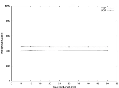
To reduce the end-to-end delay of a two-frequency wireless chain network, the time slot length should be kept small. However, a small time slot length means more frequent frequency channel and communication partner swapping operations, and this may lower the forwarding throughput of a two-frequency wireless chain network. To find out how time slot lengths may affect the forwarding throughput of a two-frequency wireless chain network, we ran two tests. In test 1, a greedy UDP flow is used. In test 2, a greedy TCP flow is used. The results of test 1 and test 2 are plotted together inFig. 9.

Fig. 6. The throughputs of a greedy UDP (test 1) or TCP (test 2) flow under the IEEE 802.11 and two-frequency scheme, tested under various hop numbers. (The time slot length in the two-frequency scheme is 10 ms).

From the figure, we see that even when the time slot length is shortened to only 5 ms, the UDP and TCP throughputs are still as good as those when the time slot lengths are large. This good property is due to the design’s using no control packet handshaking during the channel swapping process.

5.6. Bit error rate issue

With a non-zero BER, frames may be corrupted and lost. By assuming that bit errors are uniformly distributed over the bits of a packet, PER can be derived from BER and is about (BER £ m), where m is the number of bits in a packet.

To reduce the effective PER, the IEEE 802.11 scheme may retransmit a long frame at the MAC layer up to four times if its MAC-layer ACK frame does not come back. This reduces the effective PER to ðBER £ mÞ4: The end-to-end PER of an IEEE 802.11 wireless chain network with N hops thus can be modeled as N £ ðBER £ mÞ4:

In the two-frequency scheme, most frames are retrans-mitted (if necessary) using the IEEE 802.11 scheme. This means that these frames’ effective PERs are as small as those in the IEEE 802.11 scheme. However, during the channel swapping process, if a frame is corrupted, it may not be retransmitted in the optimistic mode because this mode has the ‘at most once’ semantic for new data frames. These Fig. 7. The throughputs of two greedy UDP (test 1) or TCP (test 2) flows when they compete in opposite directions on a two-frequency wireless chain network, tested under various hop numbers. (The time slot length is 10 ms).

frames’ effective PERs thus are ðBER £ mÞ and higher than their effective PERs in the IEEE 802.11 scheme. Because the effective PERs of these frames are higher than those of the other frames in the two-frequency scheme, we call these frames ‘fragile frames’ in the following discussion.

Due to these fragile frames, the end-to-end PER of a two-frequency wireless chain network that uses the optimistic mode is higher than that of an IEEE 802.11 wireless chain network. However, the simulation results show that UDP and TCP still achieve much higher throughputs on a two-frequency wireless chain network than on an IEEE 802.11 wireless chain network, unless the BER is excessively high. The reason is that an IEEE 802.11 wireless chain network has the serious 1=N low forwarding throughput problem for both UDP and TCP traffic. In contrast, the two-frequency wireless chain network does not have this problem.

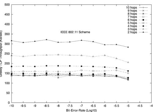
Figs. 10 and 11 show the achieved throughputs of a greedy UDP flow on an IEEE 802.11 and a two-frequency wireless chain network, respectively. Parameters varied are the BER and the hop number. Because UDP load is not sensitive to packet losses, a non-zero BER (PER) does not hurt its performance much. Clearly, we see that the two-frequency scheme outperforms the IEEE 802.11 scheme for UDP traffic.

Figs. 12 and 13 show the achieved throughputs of a greedy TCP flow on an IEEE 802.11 and a two-frequency wireless chain network, respectively. Parameters varied are the BER and the hop number. Because TCP load is sensitive to packet losses, a network with a non-zero BER (PER) may unnecessarily trigger its congestion control and thus hurt its performance. By comparing the two figures, we see that in most conditions the two-frequency scheme outperforms

the IEEE 802.11 scheme for TCP traffic. The two-frequency scheme performs worse than the IEEE 802.11 scheme only in the high BER and few hop region (where BER is between 1025.5and 1025and the hop number is 2 and 3).

We note that reducing the BER of a wireless link or the effective PER of a transmitted frame can be done in many ways (e.g. by placing the sending and receiving stations closer to each other, using error-correcting codes, or increasing the transmit power). However, the 1=N low forwarding throughput problem cannot be cost-effectively solved without using the two-frequency scheme.

5.7. Operating mode issue

Here we compare the performances of the optimistic and pessimistic modes of the two-frequency scheme. We will show how UDP and TCP perform in these modes. On one hand, because the optimistic mode has a higher end-to-end effective PER than the pessimistic mode, TCP in the optimistic mode may have a worse performance than in the pessimistic mode. On the other hand, the pessimistic mode may generate duplicate frames, which may hurt TCP performance as well. It is interesting to see which mode can provide a higher throughput for a greedy TCP flow in most conditions.

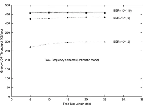
Fig. 14shows the achieved throughputs of a greedy UDP flow on a two-frequency wireless chain network that uses the optimistic mode, under various combinations of time slot length and BER.Fig. 15shows the performances of the same test except that now the operating mode is set to the pessimistic mode. From these figures, we see that because UDP is sensitive to neither packet losses nor packet Fig. 9. The throughputs of a greedy UDP (test 1) or TCP (test 2) flow on a two-frequency wireless chain network, tested under various time slot lengths. (The number of hops of the wireless chain network is 10).

duplications, these two modes have similar UDP performances.

Fig. 16shows the achieved throughputs of a greedy TCP flow on a two-frequency wireless chain network that uses the optimistic mode, under various combinations of time slot length and BER.Fig. 17shows the performances of the same test except that the operating mode now is set to the pessimistic mode. The results show that the optimistic mode can provide a much higher forwarding throughput for TCP traffic than the pessimistic mode.

The results are somewhat surprising. Most people would guess that the pessimistic mode could give TCP a better performance for the following reasons. First, TCP is very sensitive in the sense that any TCP data packet loss will trigger TCP congestion control. Since the PER of the pessimistic mode is much less than the PER of the optimistic mode, TCP should perform better in the pessimistic mode. Second, TCP is relatively insensitive to packet duplications because receiving less than three duplicate TCP ACK packets will not trigger TCP congestion control. As such, Fig. 10. The throughput of a greedy UDP flow on an IEEE 802.11 wireless chain network, tested under various combinations of BERs and hop numbers.

Fig. 11. The throughput of a greedy UDP flow on a two-frequency wireless chain network, tested under various combinations of BERs and hop numbers. (The time slot length is 10 ms).

even if a frame may be duplicated in the pessimistic mode, these duplicated frames should not hurt TCP performance too much.

Although the above qualitative arguments are correct, we found that the surprising results actually are caused by the fact that the packet loss probability in the optimistic mode is much smaller than the packet duplication probability in the pessimistic mode. In the optimistic mode, the last frame transmitted in a time slot will be lost only when both of the following two conditions hold. First, the last frame’s ACK

frame has not been received when a channel swapping command is issued. Second, bit errors really occur and corrupt this frame (the probability of this condition is PER). However, in the pessimistic mode, the last frame transmitted in a time slot will be duplicated simply when the above first condition holds. The packet loss probability in the optimistic mode thus is 1/PER times smaller than the packet duplication probability in the pessimistic mode. As an example, suppose that BER is 10210 and thus PER is (10210£ 12,000) for 1500 byte frames, the ratio of Fig. 12. The throughput of a greedy TCP flow on an IEEE 802.11 wireless chain network, tested under various combinations of BERs and hop numbers.

Fig. 13. The throughput of a greedy TCP flow on a two-frequency wireless chain network, tested under various combinations of BERs and hop numbers. (The time slot length is 10 ms).

the packet duplication probability in the pessimistic mode over the packet loss probability in the optimistic mode is a very large number of 8.3 £ 105

5.8. Clock synchronization issue

In Section 4.2 when we presented the two-frequency scheme, we implicitly assumed that the clocks of the stations on a wireless chain network are all reasonably

synchronized. This assumption is reasonable. In Ref.[1], it is stated that, because beacons (which carry clock information) are broadcast in an ad hoc network, the accuracy of 802.11 stations’ clocks shall be within 0.01%.

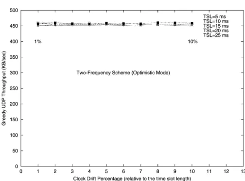
Even if the above statement is not supported, the following results show that precise clock synchronization is not needed in the two-frequency scheme.Fig. 18shows the throughputs of a greedy UDP flow on a two-frequency wireless chain network, under various combinations of Fig. 14. The throughput of a greedy UDP flow on a two-frequency wireless chain network (the optimistic mode), tested under various combinations of time slot lengths and BERs. (The number of hops is 10).

Fig. 15. The throughput of a greedy UDP flow on a two-frequency wireless chain network (the pessimistic mode), tested under various combinations of time slot lengths and BERs. (The number of hops is 10).

time slot length and clock drift percentage. We use the clock drift percentage to add random offsets to a station’s original channel swapping times (i.e. the times when the channel swapping command should be issued by the station’s timer). If the clocks of these stations are precisely synchronized and there is no clock drift, each station’s original channel swapping time for time slot ðiÞ should be time_slot_length £ ði 2 1Þ: In order to simulate the effect of clock drift, for every station’s every time

slot, we draw a random number uniformly between [2 time_slot_length £ clock_ drift_percentage, þ time_ slot_length £ clock_drift_percentage] and add it to the time slot’s original channel swapping time. By increasing the clock drift percentage, we can make the stations’ clocks less and less synchronized.

The results show that inaccurate clock synchronization does not hurt the performance of the two-frequency scheme. Under various time slot lengths, a clock drift percentage up Fig. 16. The throughput of a greedy TCP flow on a two-frequency wireless chain network (the optimistic mode), tested under various combinations of time slot lengths and BERs. (The number of hops is 10).

Fig. 17. The throughput of a greedy TCP flow on a two-frequency wireless chain network (the pessimistic mode), tested under various combinations of time slot lengths and BERs. (The number of hops is 10).

to 10% still does not hurt the two-frequency scheme’s performance.

6. Future work

The two-frequency scheme was originally proposed for fixed wireless chain networks. However, after some modifications, it can also be extended to support two-dimensional lattice networks or mobile ad hoc networks. In the following, the proposed extensions are presented and left as our future work.

6.1. Lattice networks

If we properly configure each station’s frequency channel and communication partner swapping schedule, the two-frequency scheme can be used in a lattice network to provide a two-dimension coverage area.

Unlike a wireless chain network, which alternates between two different patterns, a lattice network will cycle through four different patterns in consecutive time slots to provide horizontal and vertical communications.

Fig. 19 shows a possible schedule for a 7 £ 7 lattice network, where (a), (b), (c), and (d) represent the four different patterns. In the figure, a thick link between station ðiÞ and station ðjÞ means that station ðiÞ and station ðjÞ are each other’s communication partner in that pattern, and the number above or next to the thick link represents the frequency channel used in that pattern. Using this schedule, a dark node need not change it frequency channel, a gray node needs to change it channel between two different

channels, and all the other nodes need to change their channels among four different channels. Because now a station has four different communication partners, it uses four output queues in its wireless NIC.

During the time slots using pattern (a) and (b), packets can (and can only) be forwarded horizontally. During the time slots using pattern (c) and (d), instead, packets can (and can only) be forwarded vertically. Because the sequence of the patterns used by consecutive time slots is (a, b, c, d, a, b, c, d,…), a packet can be forwarded from any station to any other station through multiple hops on a lattice network.

When the traffic on a lattice network is greedy cross traffic, the two-frequency scheme can have a 300% throughput improvement over the normal IEEE 802.11 scheme. In Ref.[3], the authors have shown that if on each row and column of the lattice network there is a greedy flow (represented by a long line with an arrow in the figure), the maximum throughput that each flow can simultaneously achieve is 1/12 in the normal IEEE 802.11 scheme. In the two-frequency scheme, because the signal interrence problem does not exist, we can see that the maximum throughput that each flow can simultaneously achieve is 1/4. Because a wireless NIC is half-duplex and a station needs to forward its horizontal and vertical flows’ packets, 1/4 (which equals (1/2)/2) is already the optimal throughput that each flow can simultaneously achieve under this greedy cross traffic configuration.

The proposed schedule statically allocates 50% and 50% of a wireless NIC’s bandwidth to its horizontal and vertical traffic, respectively. If the traffic on the lattice is uneven or if the traffic is sparse (i.e. at any time, there are only a few routing paths that are actively used to forward packets), this Fig. 18. The throughput of a greedy UDP flow on a two-frequency wireless chain network (the optimistic mode), tested under various combinations of time slot lengths and clock drift percentage. (The number of hops is 10).

static schedule may unnecessarily waste some time slots (bandwidth). In this case, using an on-demand signaling protocol to dynamically configure involved stations will provide higher forwarding bandwidth for these active routing paths. We discuss the signaling protocol issue in Section 6.2.

6.2. Mobile ad hoc networks

Once set up, the frequency channel and communication partner swapping schedule can be easily maintained and used for a long time in fixed multi-hop wireless networks. Therefore, the two-frequency scheme is well suited for fixed multi-hop wireless networks. For a mobile ad hoc network, because stations may move and thus its network topology may change, an on-demand signaling protocol is needed to dynamically create and maintain swapping schedules for the stations on an active routing path. In the following, we propose a simple signaling scheme as the first step toward designing a more efficient, robust, and complete signaling scheme for mobile ad hoc networks.

Initially, all stations in a mobile ad hoc network use a default frequency channel to communicate. This frequency channel is also the channel that will be used by the signaling protocol. The signaling protocol can be combined with an on-demand routing protocol such as the AODV[12]or the DSR[13] routing protocol. After the routing protocol has found a routing path, it can immediately execute the signaling protocol. The signaling protocol will then issue a control packet to configure the involved stations on the routing path.

If the traffic in a mobile ad hoc network is sparse such that at any time no active routing path intercepts with other active routing paths, the signaling protocol can use the swapping schedule designed for a wireless chain network to configure the stations on an active routing path. If the traffic is dense such that two active routing paths intercept with each other at some station, the signaling protocol can use the swapping schedules designed for a horizontal line and a vertical line in a lattice network to configure the stations on these two routing paths. In either case, these stations will start using the assigned frequency channels to receive, send, and forward packets.

When an active routing path becomes inactive (e.g. there is no traffic flowing on the path for a while), the swapping schedules used by the stations on the inactive routing path should be removed. Otherwise, if a new routing path is set up and the new routing path intercepts with the inactive routing path, the signaling protocol will unnecessarily use the less bandwidth-efficient lattice swapping schedules rather than the chain swapping schedules to configure the stations on the new routing path. Removing a station’s swapping schedule can be done by using the soft state technique [14]. In this technique, a state will be removed automatically after a certain period of idle time. After the swapping schedule is removed, a station will again use the default frequency channel to communicate.

If a wireless link on a routing path breaks due to station movements, the swapping schedules used by the other stations that are still on the routing path may need to be reconfigured. The reconfiguration procedure can be trig-gered by the routing protocol automatically as the routing Fig. 19. The four different frequency channel and communication partner swapping patterns used for a lattice network.

protocol will detect the path failure and re-initiate its route-finding operation.

In the two-frequency scheme, stations on an active routing path may be configured to use a frequency channel that is different from the default channel to forward packets. To ensure that every station is able to receive signaling packets, stations’ clocks will need to be synchronized and stations will need to periodically switch their frequency channels back to the default channel in certain reserved time slots. These reserved time slots will not be used by the two-frequency scheme for forwarding packets. If a station has signaling packets to send or forward (including the routing protocol’s packets because they are also used for the signaling purpose), these packets should also be sent in these time slots.

Because the topology of a mobile ad hoc network may change constantly, to handle all possible situations well, the proposed signaling scheme will definitely need to be refined. Here, we just present a crude but feasible scheme. Designing a better signaling scheme is our future work.

Note that because the topology of a mobile ad hoc network may change constantly, the assumption made in Section 4.2.1 that neighboring stations are D meters apart, where ð550=3Þ , D , 250; may not always hold. Therefore, the optimal forwarding performance (i.e. 1/2) achieved by the two-frequency scheme represents only an upper bound in a mobile ad hoc network. The real achieved performance may be less than the optimal performance.

7. Conclusions

In this paper, we address an important problem with wireless chain networks. On a N-hop wireless chain network, when a stream of packets is forwarded, exper-imental and simulation results both show that, regardless of the transport protocol (e.g. TCP or UDP) used, the stream’s achieved throughput is only 1=N (of the wireless bandwidth) when N is less than 5 and stabilize at 1/5 or even less when N becomes large. Because the chain topology is a basic topology and commonly used, the 1=N low forwarding throughput problem is important. To solve this problem, we propose the two-frequency scheme. In this scheme, every station swaps its frequency channel between two different channels and swaps its communication partner between its two neighboring stations in consecutive time slots. The forwarding throughput of a N-hop wireless chain network in the proposed scheme is improved from 1=N to 1/2, given any N: Since 1/2 is the maximum forwarding throughput achievable by a half-duplex wireless interface, the two-frequency scheme cost-effectively optimizes the forwarding throughput of a N-hop wireless chain network.

Acknowledgements

We would like to thank the anonymous reviewers for their valuable comments. This research was supported in part by MOE Program for promoting Academic Excellence of Universities under the grant number 89-E-FA04-1-4 and 91-E-FA06-4-4, the Lee and MTI Center for Networking Research, NCTU, the Institute of Applied Science and Engineering Research, Academia Sinica, Taiwan, and NSC grant 91-2213-E-009-064.

References

[1] IEEE Computer Society LAN MAN Standards Committee, Wireless LAN Medium Access Control (MAC) and Physical Layer (PHY) Specifications, IEEE Std 802.11-1999. The institute of Electrical and Electronics Engineering, New York, 1999.

[2] G. Holland, N. Vaidya, Analysis of TCP performance over mobile ad hoc networks, ACM MOBICOM’99, Seattle, Washington, USA August (1999).

[3] J. Li, C. Blake, D.S.J. De Couto, H.I. Lee, R. Morris, Capacity of ad hoc wireless networks, ACM MOBICOM’01, Rome, Italy July (2001).

[4] M. Gerla, K. Tang, R. Bagrodia, TCP performance in wireless multi-hop networks, IEEE WMCSA’99, New Orleans, LA, USA February (1999).

[5] K. Tang, M. Gerla, Fair sharing of MAC under TCP in wireless ad hoc networks, IEEE MMT’99, Venice, Italy October (1999).

[6] M. Gerla, R. Bagrodia, L. Zhang, K. Tang, L. Wang, TCP over wireless multi-hop protocols: simulation and experiments, IEEE ICC’99, Vancouver, Canada June (1999).

[7] R. Bagrodia, R. Meyer, M. Takai, Y.A. Chen, X. Zeng, J. Martin, H.Y. Song, PARSEC: a parallel simulation environment for complex system, Computer Magazine (1998).

[8] K. Fall, K. Varadhan, ns Notes and Documentation, LBNL Technical Report, August 1998,http://www-mash.cs.berkeley.edu/ns/. [9] S.Y. Wang, C.L. Chou, C.H. Huang, C.C. Hwang, Z.M. Yang, C.C.

Chiou, C.C. Lin, The Design and Implementation of the NCTUns 1.0 Network Simulator, Computer Networks Journal, in press. (The NCTUns 1.0 network simulator software is available athttp://NSL. csie.nctu.edu.tw/nctuns.html).

[10] T.S. Rappaport, Wireless Communication: Principle and Practice, Prentice Hall, Englewood Cliffs, NJ, 1996, pp. 85 – 90.

11 R. Garces, J.J. Garcia-Luna-Aceves, Collision avoidance and resolution multiple access for multichanel wireless N networks, IEEE INFO-COM’2000, Tel-Aviv, Israel March (2000).

[12] C. Perkins, E. Royer, Ad hoc on demand distance vector routing, Second IEEE Workshop on Mobile Computing Systems and Applications February (1999).

[13] D.B. Johonson, Routing in ad hoc networks of mobile hosts, First IEEE Workshop on Mobile Computing Systems and Applications December (1994).

[14] S. Roman, S. McCanne, A model, analysis, and protocol framework for soft state-based communication, ACM SIGOCMM’99, Harvard University August (1999).