Bayesian inference in joint modelling of location and scale parameters of the t distribution for longitudinal data

Bayesian inference in joint modelling of location and

scale parameters of the t distribution for longitudinal

data

Tsung-I Lin

⋆, Wan-Lun Wang

a_{Institute of Statistics, National Chung Hsing University, Taichung 402, Taiwan} b_{Department of Applied Mathematics, National Chung Hsing University, Taichung}

402, Taiwan

c_{Department of Public Health, China Medical University, Taichung 404, Taiwan} d_{Department of Statistics, Feng Chia University, Taichung 40724, Taiwan}

Abstract

This paper presents a fully Bayesian approach to multivariate t regression models whose mean vector and scale covariance matrix are modelled jointly for analyzing longitudinal data. The scale covariance structure is factorized in terms of unconstrained autoregressive and scale innovation parameters through a modi-fied Cholesky decomposition. A computationally flexible data augmentation sampler coupled with the Metropolis-within-Gibbs scheme is developed for computing the posterior distributions of parameters. The Bayesian predictive inference for the fu-ture response vector is also investigated. The proposed methodologies are illustrated through a real example from a sleep dose-response study.

Key words: Cholesky decomposition; Data augmentation; Deviance information

cri-terion; Maximum likelihood estimation; Outliers; Predictive distribution.

⋆ Corresponding author. Tel.: +886-4-22850420; fax: +886-4-22873028. E-mail address: tilin@amath.nchu.edu.tw (T.I. Lin)

1. Introduction

During the last decade, methods of joint mean-covariance estimation for general linear models based on the modified Cholesky decomposition have received consid-erable attention in the literature (see, e.g., Pourahmadi, 1999) as a powerful tool for analyzing nonstationary longitudinal data. The key features with such an ap-proach can be attributed to the facts that the covariance matrix is constrained to be nonnegative definite and has a statistically meaningful unconstrained parameteriza-tion. Pourahmadi (2000) provided a fast scoring method for obtaining the maximum likelihood (ML) estimates of unconstrained parameters and recommended using the Bayesian Information Criterion (BIC) to select the optimal model. Pan and MacKen-zie (2003) later provided a data-driven technique for efficiently finding the global optimum of selected models. Recently, Cepeda and Gamerman (2004) presented a fully Bayesian approach to fitting this class of models via a generalization of the Metropolis-Hastings (M-H) algorithm (Hastings, 1970) of Cepeda and Gamerman (2000).

It is well known that statistical modelling built on the normality assumption tends to be vulnerable to the presence of outliers. In contrast, the multivariate t distribution has been recognized as a useful generalization of the normal distribu-tion for robust inferences. For instance, Lange et al. (1989) introduced t-distributed regression model as a straightforward extension of the normal one. Pinheiro et al. (2001) considered a robust approach to linear mixed models (Larid and Ware, 1982) by assuming that both random effects and within-subject errors follow a multivariate

t distribution. Further developments for analyzing multi-outcome longitudinal data

in the context of multivariate t linear mixed models were considered by Wang and Fan (2010), among others. A Bayesian analysis of t linear mixed models of Pinheiro et al. (2001) was investigated by Lin and Lee (2007). Recently, Lin and Wang (2009) adopted a t-based joint modelling of mean and scale covariance for the analysis of

longitudinal data and demonstrated its robustness through several real examples. A d-dimensional random vector Y is said to follow a multivariate t distribution with location vector µ, scale covariance matrix Σ and degrees of freedom ν, denoted by Y ∼ Td(µ, Σ, ν), if its density function is given by

f (Y ) = Γ ( (ν + d)/2) Γ(ν/2)(πν)d/2|Σ| −1/2 [ 1 + (Y − µ) T_Σ−1_(Y − µ) ν ]_−(ν+d)/2 .

The mean and covariance matrix of Y are µ (ν > 1) and νΣ/(ν − 2) (ν > 2), respectively. If ν → ∞, then the distribution of Y reduces to Nd(µ, Σ). Liu and

Rubin (1995) offered some efficient EM-type algorithms for ML estimation of mul-tivariate t distributions. For a comprehensive introduction to fundamental theories and characterizations of the multivariate t distribution along with its applications, the reader is referred to the monograph of Kotz and Nadarajah (2004).

With the fast development of Markov chain Monte Carlo (MCMC) methods, the Bayesian sampling-based approach has become an attractive alternative for drawing richer inferences. The advantages of adopting Bayesian methods involve the incor-poration of prior information and the interpretation of parameters uncertainties. Bayesian inference often involves computing moments or quantiles of the posterior distribution, however, it requires a large amount of integration tasks. Typically, it is difficult to obtain the marginal posterior distributions by adopting the multidi-mensional integration. To address this issue, the MCMC method has been shown the most feasible tool from many important problems encountered in practice. In a Bayesian paradigm, the posterior inference can be accurately extracted from a large set of converged MCMC samples.

In this paper, we develop an efficient data augmentation (DA) sampler (Tanner and Wong, 1987) coupled with the idea of Metropolis-within-Gibbs scheme (Tier-ney, 1994) for implementing the Bayesian treatment of models proposed by Lin and Wang (2009). The priors are chosen to be weakly informative to avoid improper posterior distributions. Moreover, the selected prior distributions are conditionally

conjugate, which are very convenient when implementing the MCMC algorithm. Posterior predictive inferences for future values are also addressed.

The rest of the paper is organized as follows. In the next section, we formulate the model and review some of its relevant properties. In Sections 3, we present a full Bayesian inference for marginal posterior distributions as well as the predictive distribution of future observations. The proposed methodologies are illustrated with a real data set in Section 4 and a brief conclusion is given in the final section.

2. Model and estimation

Suppose there are N subjects in a longitudinal study. Let Yi = (Yi1, . . . , Yini)

T

be the vector of ni measurements on the ith subject collected at the time points

ti = (ti1, . . . , tini) T_{, and X} i = [ xi1 · · · xini ]T

be an ni× p design matrix, where

xij is a p× 1 vector of covariate corresponding to Yij.

The model considered here is

Yi ∼ Tni(µi, Σi, ν) (i = 1, . . . , N ), (1)

where µ_i = (µi1, . . . , µini)

T _{is the mean response vector for subject i. Following}

Pourahmadi (1999), we reparameterize Σi via the modified Cholesky decomposition

as

LiΣiLTi = Di, (2)

where Di = diag{σ12, . . . , σ2ni} and Li = [ℓjk] is a unit lower triangular matrix with the (j, k)th entry being −ϕjk. It follows immediately that Σ−1i = L

T

i D−1i Li. The

parameters ϕjk and σj2 in Li and Di are referred to as the autoregressive parameters

and scale innovation variances of Σi, respectively. Statistical interpretations for such

the autoregressive parameters, namely −ϕjk, in ˆ Yij = µij + j_∑−1 k=1 ϕjk(Yik− µik),

which is the linear least squares predictor of Yij based on its predecessors; (b) the

diagonal entries of Di are the scale innovation variances σj2 = c−1ν var(Yij − ˆYij),

where cν = ν/(ν− 2).

To make the dimension of unconstrained parameters µij, ϕjk and log σ2j more

parsimonious, we model them using covariates in the spirit of Pourahmadi (1999), namely, for j = 1 . . . , ni and k = 1, . . . , j− 1,

µij = xTijβ, log σ

2

j = w

T

jλ, ϕjk = zTjkγ, (3)

where β, λ and γ are p× 1, q × 1 and d × 1 vectors of unknown and unrestricted parameters, respectively. Note that wj and zjk are q × 1 and d × 1 parsimonious

covariate vectors, which can usually be determined in terms of polynomial of mea-surement times tij’s with degrees of q−1 and d−1, respectively. Note that λ and γ are

assumed to be common for all Σi’s for exhibiting the same covariance structure.

Sim-ply speaking, Σi’s can be shrinkable or extendible, depending on i only through its

dimension ni× ni. Accordingly, the parameters of interest are θ = (βT, λT, γT, ν)T.

The log-likelihood function for the observed data Y = (Y1, . . . , YN) is given by

ℓ(θ|Y ) = N ∑ i=1 log Γ ( ν + ni 2 ) − N log Γ(ν 2 ) − n 2log(πν)− 1 2 N ∑ i=1 ni ∑ j=1 wT_jλ −1 2 N ∑ i=1 (ν + ni) log ( 1 + ∆i(β, γ, λ) ν ) , where ∆i(β, λ, γ) = (Yi − Xiβ)TΣ−1i (Yi − Xiβ) and n = ∑_N

i=1ni is the total

number of observations. The ML estimates ˆθ are obtained as

ˆ

θ = argmax θ

which generally have no analytical solution. Lin and Wang (2009) provided a fast scoring algorithm for carrying out ML estimation with the standard errors as a by-product.

It follows from the essential property of the multivariate t distribution that

Yi ∼ Tni(µ, Σ, ν) can be hierarchically expressed as Yi | τi ∼ Nni (

µ, τ_i−1Σ) and

τi ∼ Γ(ν/2, ν/2), where Γ(α, β) stands for a gamma distribution with mean αβ−1.

Writing τ = (τ1, . . . , τn), the complete data likelihood function is expressed as

Lc(θ| Y , τ ) ∝ exp { − 1 2 N ∑ i=1 (∑ni j=1 wT_i λ + τi ( ν + ∆i(β, λ, γ) ))} × [ (ν/2)ν/2 Γ(ν/2) ]_{N N} ∏ i=1 τ(ν+ni−2)/2 i , (4) where |Di| = |Li||Σi||LTi | = |Σi|, ri = Yi − Xiβ = {rij}nj=1i and ∆i(β, λ, γ) =

(ri−Ziγ)TD−1i (ri−Ziγ) with Zi = [z(i, 1) · · · z(i, ni)]Tand z(i, j) =

∑j−1

k=1rikzjk.

The ECME algorithm (Liu and Rubin, 1994), a generalization of EM (Dempster et al., 1977), extends the ECM algorithm of Meng and Rubin (1993) with the CM-steps by maximizing either the expected complete data log-likelihood function or the correspondingly constrained actual log-likelihood function, called the ‘CML-step’. The main advantage of the ECME algorithm is that it not only preserves the nice features of EM and ECM, but also converges substantially faster than EM and ECM, as demonstrated by Liu and Rubin (1995) for ML estimation of multivariate

t distribution with unknown degrees of freedom. Instead of the scoring method

employed in Lin and Wang (2009), a computationally efficient ECME algorithm for obtaining the ML estimates ˆθ in this context is given in a longer version of this

3. Bayesian Methodology

3.1. Prior settings, full conditionals and the DA sampler

To accomplish a Bayesian setup of the model, one must specify a prior distribu-tion for the parameter θ = (βT, λT, γT_{, ν)}T_{. Assuming that the prior distributions}

of β, λ, γ and ν are independent a priori, the joint prior density is

π(θ)∝ π(β)π(λ)π(γ)π(ν).

When there is no prior information about θ, a convenient strategy of avoiding improper posterior distribution is to use diffuse proper priors. In this case, the posterior inference will be very close to those obtained by the ML method for large samples. In many circumstances, the Bayesian approach is more useful for situations in which the large sample properties cannot be applied for ML inference, especially when the collected samples are not sufficient enough.

The prior specifications adopted here are as follows:

β∼ Np(µβ, Σβ), λ∼ Nq(µλ, Σλ),

γ∼ Nd(µγ, Σγ), log (1/ν)∼ U(−10, 10), (5)

where the hyperparameters µ_β, µ_λ, µ_γ, Σβ, Σλ and Σγ are assumed to be known

quantities. Typically, µ_β, µ_λ and µ_γ are zero vectors. To reflect the prior indepen-dence among β, λ and γ, the structures of Σβ, Σλand Σγ can be taken as diagonal

matrices with relatively large numbers on the main diagonal. In the later analysis, we take Σβ = 104Ip, Σλ = 104Iq and Σγ = 104Id for ensuring a reasonably flat

prior distribution for β, λ and γ. Note that the prior for ν in (5) follows that em-ployed in Liu and Rubin (1998) on the basis of vagueness.

Multiplying the complete data likelihood function (4) with the prior distribu-tions in (5), the joint posterior distribution of (β, λ, γ, ν, τ ) is given by

p(β, λ, γ, ν, τ | Y ) ∝ exp{−1 2 N ∑ i=1 (∑ni j=1 wT_i λ + τi ( ν + ∆i(β, λ, γ) ))}_∏N i=1 τ(ν+ni−2)/2 i × [ (ν/2)ν/2 Γ(ν/2) ]N exp { − 1 2(β− µβ) T_Σ−1 β (β− µβ) } × exp{−1 2(λ− µλ) T_Σ−1 λ (λ− µλ)− 1 2(γ− µγ) T_Σ−1 γ (γ − µγ) } Jν, (6)

where Jν = 1/ν(0 < ν <∞) is the Jacobian of transforming log (1/ν) to ν.

The DA algorithm introduced by Tanner and Wong (1987) has been shown to be a powerful tool for the computation of the entire posterior distribution. The key idea behind the algorithm is to augment the observed data Y to the latent vector τ . The DA algorithm consists of the imputation step (I-step) and the posterior step (P-step). At the kth iteration, the I-step imputes the missing data by drawing τ_i(k) from the predictive distributions p(τi | Y , θ(k)). The P-step refers to generating θ(k+1)

from p(θ | Y , τ_i(k+1)). Under suitable regularity conditions, the simulated samples of τ_i(k)’s and θ(k)converge to their associated target distributions after a sufficiently long burn-in period.

The following proposition provides the required conditional posterior distribu-tions used in the DA algorithm.

Proposition 1. From (6), the full conditionals are given as follows (the notation

“| · · · ” denotes conditioned on Y and all other variables):

τi | · · · ∼ Γ ( ni+ ν 2 , ν + ∆i(β, λ, γ) 2 ) , (7) β| · · · ∼ Np(b∗, B∗), (8) γ| · · · ∼ Nd(g∗, G∗), (9) where

b∗= B∗ ( Σ−1_β µ_β+ N ∑ i=1 τiXTi Σ−1i Yi ) , B∗= ( Σ−1_β + N ∑ i=1 τiXTi Σ−1i Xi )₋₁ , g∗= G∗ ( Σ−1_γ µ_γ + N ∑ i=1 τiZTi D−1i ri ) , G∗= ( Σ−1_γ + N ∑ i=1 τiZTi D−1i Zi )₋₁ .

The full conditional distributions of λ and ν given below are not of standard forms.

p(λ| · · · ) ∝ exp{−1 2 N ∑ i=1 (∑ni j=1 wT_i λ + τi∆i(β, λ, γ) ) − 1 2(λ− µλ) T_Σ−1 λ (λ− µλ) } (10) and p(ν | · · · ) ∝ [ (ν/2)ν/2 Γ(ν/2) ]N(_∏N i=1 τ_iν/2 ) exp { −ν 2 N ∑ i=1 τi } Jν. (11)

Proof: The proof follows from standard calculations and hence is omitted.

In the simulation process, samples for τi’s and θ are alternately generated. In

summary, the implementation of DA algorithm proceeds as follows:

I-Step: Impute τi from its conditional posterior in (7) for i = 1, . . . , N .

P-Step:

1. Draw β from its full conditional posterior in (8). 2. Draw γ from its full conditional posterior in (9). 3. Update λ from (10) via the M-H algorithm. 4. Update ν from (11) via the M-H algorithm.

To elaborate on P -Step 3 of the above algorithm, a multivariate normal distri-bution Nq(λ(k), c2Iˆ

−1

λλ) is chosen as the random walk jumping distribution J ( ˜λ|λ

(k)

), where the scale c can be taken around 2.4/√q (Gelman et al., 1996). Moreover, ˆI−1_λλ

information matrix of λ is Iλλ = 1 2 N ∑ i=1 ν + ni ν + ni+ 2    ni ∑ j=1 wjwTj − ( ∑ni j=1wj )( ∑ni j=1wTj ) ν + ni   .

Because the proposal distribution is symmetric, it follows from the Metropolis jump-ing rule (Metropolis et al., 1953) that

λ(k+1) =          ˜

λ with probability min{1, α}, λ(k) otherwise, where α = p( ˜λ| β (k+1) , γ(k+1), ν(k), τ(k+1), Y ) p(λ(k) | β(k+1), γ(k+1)_{, ν}(k)_{, τ}(k+1)_{, Y )}.

For sampling ν in P -Step 4, we first transform ν to ν∗ = log (1/ν) and then apply the M-H algorithm to the function g(ν∗ | · · · ) = p(ν(ν∗) | · · · )e−ν∗. The jumping distribution J (ν∗(k+1)|ν∗(k)) can be chosen as a truncated normal distribu-tion with mean ν∗(k) and variance 2.42σˆ_ν2∗ before truncation, and truncated region A = (−10, 10), where ˆσ2

ν∗ = ˆν−2Iˆν−1 and ˆIν−1 is the inverse information matrix of ν

evaluated at ˆν. Note that Iν is given as Iν = 1 4 N ∑ i=1 { ψ ( ν 2 ) − ψ ( ν + ni 2 ) − 2ni(ν + ni+ 4) ν(ν + ni)(ν + ni+ 2) } ,

where ψ(x) = d2_{log Γ(x)/dx}2 _{is the trigamma function. Notably, at the (k + 1)st}

iteration, one can generate a truncated normal variate (Gelfand et al., 1992) by

ν∗(k+1) = ν∗(k)+σν(k)∗Φ−1   Φ (_{−10 − ν∗}(k) σ_ν(k)∗ ) + U [ Φ ( 10− ν∗(k) σ_ν(k)∗ ) − Φ(−10 − ν∗ (k) σ_ν(k)∗ )]_ , where Φ(·) denotes the cumulative distribution function of N(0, 1) and U denotes a random uniform (0, 1) variate. Note that ν∗(k+1) is accepted according to the prob-ability min { 1,g(ν ∗(k+1) | · · · )J(ν∗(k) |ν∗(k+1) ) g(ν∗(k)| · · · )J(ν∗(k+1)|ν∗(k)) }

. If accepted, invert it back to ν(k+1) =

exp{−ν∗(k+1)}. Otherwise, set ν(k+1) = ν(k).

model uncertainty or any posterior inference of interest can be effectively taken into account by converged Monte Carlo samples, say{θ(k)}K_k=1. For example, an approx-imate posterior mean of θ can be estapprox-imated by ¯θ = K−1∑K_k=1θ(k) and its posterior variance-covariance can be approximated by∑K_k=1(θ(k)− ¯θ)(θ(k)− ¯θ)T/(K− 1).

3.2. Posterior predictive inference for future values

We consider the extended prediction of ˜y_i, a g× 1 future observations of Yi.

The posterior predictive density of ˜y_i is given by

p(˜y_i | Yi) =

∫

p(˜y_i | Yi, θ)p(θ | Yi)dθ. (12)

The integration in (12) is usually intractable, but can be easily approximated by constructing a set of stationary MCMC samples.

Let ˜xi be a g× p matrix of prediction regressors corresponding to ˜yi such that E(˜y_i) = ˜xiβ. Let ˜wj and ˜zjk, respectively, denote a q×1 and a d×1 covariate vector

associated with ˜y_i such that log σ2

j = ˜w

T

jλ and ϕjk = ˜zTjkγ for j = ni+ 1, . . . , ni+ g

and k = 1, . . . , j− 1. Further, we assume that the joint distribution for (YT_i , ˜yT_i )T

follows an (ni+ g)-variate t distribution, given by

     Yi ˜ y_i     ∼ Tni+g(X ∗ iβ, Σ∗i, ν) with X∗_i = (XT_i , ˜xT_i )T _{and Σ}∗−1 i = L∗Ti D∗−1i Li∗, where L∗i is a (ni + g)× (ni+ g)

lower triangular matrix having−ϕjk at the (j, k)th position, k < j, j = 1, . . . , ni+ g,

and D∗_i = diag{σ2 1, . . . , σn2i, σ 2 ni+1, . . . , σ 2 ni+g}. More specifically,

L∗_i =                        

L

0

exp(wT₁λ), . . . , exp(wT_niλ), exp( ˜w_nT_i+1λ), . . . , exp( ˜wT_ni+gλ)

}

.

Let Σ∗_i be partitioned conformably with the dimension of (YT_i , ˜yT_i )T. Therefore, we have Σ∗_i =      Σ11 Σ12 Σ21 Σ22     . (13)

Here we suppress the subscript i of the partitioned matrices in (13) for notational convenience. Note that Σ11 = Σi and Σ21 = ΣT12. Making use of the conditional

property concerning the multivariate t distribution, we have ˜ y_i | (Yi, θ) ∼ Tg ( µ_2·1,ν + ∆i(β, γ, λ) ν + ni Σ22·1, ν + ni ) , where µ_2·1 = ˜xiβ + Σ21Σ−111(Yi− Xiβ) and Σ22·1= Σ22− Σ21Σ−111Σ12.

Let θ(k) be the generated sample at the kth iteration of the DA sampler when the convergence is achieved. We can obtain the approximate predictive distribution of ˜y_i using the Rao-Blackwellization Theorem (Gelfand and Smith, 1990). That is,

p( ˜y_i | Y ) ≈ 1 K K ∑ k=1 tg ( ˜ y_i | µ(k)_2·1,ν (k)_{+ ∆} i(β(k), λ(k), γ(k)) ν(k)_{+ n} i Σ(k)_22·1, ν(k)+ ni ) , where µ(k)_2·1 = ˜xiβ(k) + Σ (k)

21Σ−1(k)11 (Yi − Xiβ(k)) and tg(˜yi | µ, Σ, ν) denotes the

4. A Numerical Illustration

Sleep is a fundamental and physiological demand of mankind. Recent investi-gations indicate that sleep deprivation and chronic sleep restriction would impact health, safety and productivity. In general, it would result in reduction of the neural behavior, irregular influence on the immune function, increased fatigue, decreased alertness and impaired performance in a variety of cognitive psychomotor tests.

As an illustration, we apply the proposed methods to the 3-hour group of a sleep dose-response study for 18 volunteer participants. They spent a total of 14 days in the Johns Hopkins Bayview General Clinical Research Center (GCRC, Baltimore, MD, USA) to complete this study. The first 2 days were adaptation and training (T1 and T2) and the third served as baseline (B). During the three days, all par-ticipants were required to be in bed from 23:00 to 07:00, i.e., 8-hour time in bed (TIB). Beginning on the fourth day, they were restricted to 3-hour TIB from 04:00 to 07:00 for the next 7 days (E1-E7). On the 11th day and lasting to the 13th day (R1-R3), they were requested 8 hours daily TIB from 23:00 to 07:00 for recovery. They are also placed a final night of 8-hour TIB to release from the study, but no testing occurred on the final recovery day (R4). The experimental design and TIB schedule are shown in Figure 1 of Belenky et al. (2003).

Of these 18 subjects, they received a series of cognitive and alterness tests, e.g., psychomotor vigilance task (PVT), polysomnography (PSG) measures and sleep latency test (SLT). The PVT is a generally acknowledged test to measure reac-tion time in ms (millisecond) to a visual stimulus, a thumb-operated and hand-held device (Dinges and Powell, 1985). Subjects heeded the LED timer display on the device and pressed the response button as soon as possible after the emergence of the visual stimulus. The group performed the PVT test four times per day (09:00, 12:00, 15:00 and 21:00). In this example, the response variable Yij is the average

This data set can be extracted from the database of lme4 R-package (Bates, 2007). A detailed description of participants, design and procedures of the study can be found in Balkin et al. (2000), Belenky et al. (2003) and Balkin et al. (2004).

Table 1 about here

Table 1 lists the sample variances and correlations among the repeated measure-ments of the data. Apparently, the variances tend to increase across time after the baseline. Furthermore, the correlations exhibit an irregular pattern within the same lagged times, suggesting that the data have a non-stationary covariance structure.

Figure 1 about here

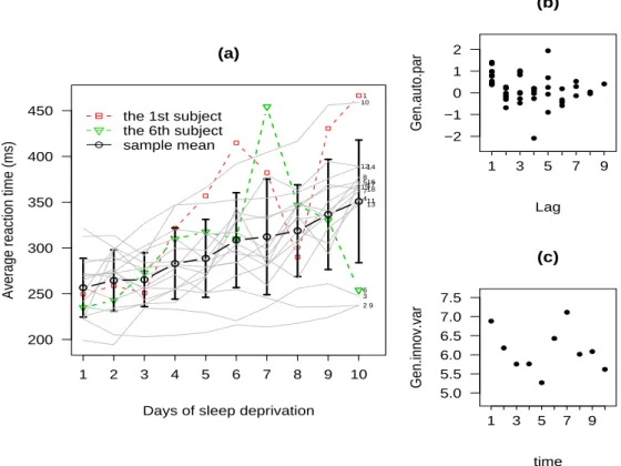
Figure 1(a) displays the trajectories of average reaction times evolved over an equally spaced 10-day period along with its mean profile and±1 standard deviations across days. A few of subjects appear to have sudden jumps and drops in experi-mental days and hence are suspected to be discordant outliers. This indicates that normal-based models could be inappropriate for this data set.

For the specification of design matrices, because the trend of population mean profile evolves linearly over time, it is reasonable to use a 1st-degree polynomial in time to model the mean responses. The covariates are thus taken as xij = (1, tij)T,

where tij = j for i = 1, . . . , 18 and j = 1, . . . , 10 . In addition, Figures 1(b) and

1(c) suggest that ϕjk’s and log σj2’s could be well suited to a cubic or a high-order

polynomial functions in lags. Following Pourahmadi (2000), we use the Poly(q, d) as a shorthand for imposing two distinct polynomials of lagged times j and j− k with degrees q and d for log σ2

j and ϕjk, respectively. Specifically, the covariates zjk and

wj are chosen as

wj= (1, j, j2, . . . , jq)T, j = 1, . . . , 10; k = 1, . . . , j− 1,

For parsimony, the largest degrees q and d are limited to 5. The best pair of degrees, say (q∗, d∗), will satisfy (q∗, d∗) = arg min(q,d){DIC(q, d)}.

Figure 2 about here

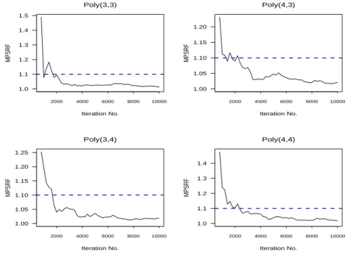
For the models fitted by MCMC sampling, we ran five parallel chains with the starting values of each chain drawn independently from their prior distributions. Based on these parallel chains, the multivariate potential scale reduction factor (MPSRF) suggested by Brooks and Gelman (1998) was used to assess the validity of convergence. Figure 2 displays the MPSRF plots for some of the selected models. Inspection of these MPSRFs suggests that the convergence occurred after 2,500 iter-ations. Therefore, we discard the first 2500 iterations for each chain as the “burn-in” samples. Furthermore, the converged MCMC realizations of each chain are collected for every 20 iterations, in order to obtain approximately independent samples. We also conduct the analysis with different values of the hyperparameters, resulting in very similar results.

Table 2 about here

Bayesian model comparison is based on the deviance information criterion (DIC) advocated by Spiegelhalter et al. (2002). The DIC is defined as

DIC = D(θ) + pD = 2D(θ)− D(¯θ) = D(¯θ) + 2pD,

where D(θ) = Eθ|Y[−2ℓ(θ | Y )] is the posterior expectation of the deviance and D(¯θ) is the deviance evaluated at the posterior means of the parameters. The penalty

term, pD = D(θ)− D(¯θ), is regarded as the effective number of parameters. Note

that the DIC can be interpreted as a Bayesian measure of fit penalized by twice the effective number of parameters pD. By definition, large value of DIC corresponds to

a poor fit. The DIC values associated with the competitive models are included in Table 2. Judging from this table, all DIC values of t models are smaller than their corresponding normal counterparts, confirming the appropriateness of the use of t

distributions. The fitted normal models are obtained by setting ν = 1, 000 when performing the MCMC algorithm. Results show that the Poly(3,4) is the preferred choice because it has the smallest DIC values for both the normal and t models.

Table 3 about here

Posterior inferences for Poly(3,4) summarized by MCMC samples, including the means, standard deviations together with 2.5% and 97.5% quantiles, are shown in Table 3. As can be seen, the 95% posterior interval of ν is (2.8, 15.1), signifying the presence of longer-than-normal errors.

Figure 3 about here

Figure 3 displays the logarithm of fitted innovation variances for the normal-and t- Poly (3,4) models along with their 95% credible intervals. In light of the graphical visualization, it appears that the t-fitted log σ2

j, which is a cubic function

of time, adapts the pattern of sample estimates more closely than does the normal one.

Figure 4 about here

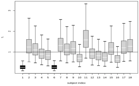
To detect possible outlying observations, Figure 4 shows the boxplots of MCMC samples of τifor i = 1, . . . , 18. As pointed out by Wakefield et al. (1994), the sampled τi’s can be used as concise indicators for detecting outliers with prior expectation of

one. When the value of τi is substantially lower than one, it gives a strong indication

that the ith participant should be regarded as an outlier in the population. Figure 4 reveals that subjects 1 and 6 are suspected outliers since none of 95% upper posterior limits exceeds 1. We marked the two subjects in colored lines in Figure 1(a). It looks fairly clear that their growth curve patterns are quite different from the others. For instance, subject 6 exhibits a sudden jump at day 6 then a sudden drop at day 7.

5. Conclusion

This paper presents a fully Bayesian approach to jointly modelling the mean and scale covariance structures for longitudinal data in the framework of multivari-ate t regression models. We have developed a workable DA sampler that enables practitioners to simulate the posterior distributions of model parameters. We also demonstrated how the model provides flexibility in analyzing heavy-tailed longitu-dinal data from a Bayesian perspective. The proposed approach allows the user to analyze real-world data in a wide variety of considerations. Numerical results illus-trated in Section 4 indicate that the t model for the sleep data is evidently more adequate than the normal one. In particular, the graphical Bayesian outputs pro-vide both easily understood inferential summaries and informative diagnostic aids for detecting outliers. Future researches along this line include a joint mean-covariance approach to multivariate skew normal models (Azzalini and Capitanio, 1999; Lin and Lee, 2008) or multivariate skew t models (Azzalini and Capitaino, 2003; Ho and Lin, 2010) to cover more possible classes or patterns for longitudinal data.

Acknowledgements

The authors would like to express their deepest gratitude to the Chief Editor, the Associate Editor and one anonymous referee for carefully reading the paper and for their great help in improving the paper. We are also grateful to Miss Wen-Chi Lin for her kind and skilful assistance in the initial simulation study. This research was supported by the National Science Council of Taiwan (Grant Nos. NSC97-2118-M-005-001-MY2 and NSC99-2118-M-035-004).

References

Azzalini, A., Capitaino, A., 1999. Statistical applications of the multivariate skew-normal distribution. J. Roy. Statist. Soc. B 61, 579–602.

Azzalini, A., Capitanio, A., 2003. Distributions generated by perturbation of sym-metry with emphasis on a multivariate skew t-distribution. J. Roy. Stat. Soc. B 65, 367–389.

Bates, D.M., 2007. lme4 R package. http://cran.r-project.org.

Belenky, G., Wesensten, N.J., Thorne, D.R., Thomas, M.L., Sing, H.C., Redmond, D.P., Russo, M.B., Balkin, T.J., 2003. Patterns of performance degradation and restoration during sleep restriction and subsequent recovery: A sleep dose-response study. J. Sleep Res. 12, 1–12.

Balkin, T.J., Thorne, D., Sing, H., Thomas, M., Redmond, D., Wesensten, N., Russo, M., Williams, J., Hall, S., Belenky, G., 2000. Effects of sleep schedules on commercial motor vehicle driver performance. Report MC-00-133, National Technical Information Service, U.S. Dept. of Transportation, Springfield, VA. Balkin, T.J., Bliese, P.D., Belenky, G., Sing, H., Thorne, D.R., Thomas, M.,

Red-mond, D.P., Russo, M., Wesensten, N.J., 2004. Comparative utility of instruments for monitoring sleepiness-related performance decrements in the operational en-vironment. J. Sleep Res. 13, 219–227.

Brooks, S.P., Gelman, A., 1998. General methods for monitoring convergence of iterative simulations. J. Comput. Graph. Statist. 7, 434–455.

Cepeda, E.C., Gamerman, D., 2000. Bayesian modeling of variance heterogeneity in normal regression models. Braz. J. Probab. Stat. 14, 207–221.

Cepeda, E.C., Gamerman, D., 2004. Bayesian modeling of joint regressions for the mean and covariance matrix. Biom. J. 46, 430–440.

Dempster, A.P., Laird, N.M., Rubin, D.B., 1977. Maximum likelihood from incom-plete data via the EM algorithm (with discussion). J. Roy. Stat. Soc. Ser. B 39, 1–38.

Gelfand, A.E., Smith, A.F.M., 1990. Sampling based approaches to calculate marginal densities. J. Am. Stat. Assoc. 85, 398–409.

Gelfand, A.E., Smith, A.F.M., Lee, T.M., 1992. Bayesian analysis of constrained parameter and truncated data problems using Gibbs sampling. J. Am. Stat. Assoc. 85, 523–532.

Gelman, A., Robert, G., Gilks. W., 1996. Efficient Metropolis jumping rules. In Bayesian Statistics 5 (Edited by J. M. Bernardo, J. O. Berger, A. P. Dawid and A. F. M. Smith). Oxford University Press, New York

Hastings, W.K., 1970. Monte Carlo sampling methods using Markov Chains and their applications. Biometrika 57, 97–109.

Ho, H.J., Lin, T.I., 2010. Robust linear mixed models using the skew t distribution with application to schizophrenia data. Biom. J. 52, 449–469.

Kotz, S, Nadarajah, S., 2004. Multivariate t Distributions and Their Applications. third ed. Cambridge University Press, New York

Lange, K.L., Little, R.J.A., Taylor, J.M.G., 1989. Robust statistical modeling using the t distribution. J. Am. Stat. Assoc. 84, 881–896.

Laird, N.M., Ware, J.H., (1982). Random effects models for longitudinal data. Biometrics 38:963–974

Lin, T.I., Lee, J.C., 2007. Bayesian analysis of hierarchical linear mixed modeling using the multivariate t distribution. J. Statist. Plann. Inference 137, 484–495. Lin, T.I., Lee, J.C., 2008. Estimation and prediction in linear mixed models with

skew normal random effects for longitudinal data. Stat. Med. 27, 1490–1507. Lin, T.I., Wang, Y.J., 2009. A robust approach to joint modeling of mean and scale

covariance for longitudinal data. J. Statist. Plann. Inference 139, 3013–3026. Liu, C., Rubin, D.B., 1994. The ECME algorithm: A simple extension of EM and

ECM with faster monotone convergence. Biometrika 81, 633–648

Liu, C., Rubin, D.B., 1995. ML estimation of the t distribution using EM and its extensions, ECM and ECME. Statist. Sinica. 5, 19–39.

Liu, C.H., Rubin, D.B., 1998. Ellipsoidally symmetric extensions of the general location model for mixed categorical and continuous data. Biometrika 85, 673– 688.

Meng, X.L., Rubin, D.B., 1993. Maximum likelihood estimation via the ECM al-gorithm: A general framework. Biometrika 80, 267–278.

Metropolis, N., Rosenbluth, A.W., Rosenbluth, M.N., Teller, A.H., Teller, E., 1953. Equation of state calculation by fast computing machines. J. Chem. Phy. 21, 1087– 1092.

Pan, J., MacKenzie, G., 2003. On modelling mean-covariance structures in longi-tudinal studies. Biometrika 90, 239–244

Pinheiro, J.C., Liu, C.H., Wu, Y.N., 2001. Efficient algorithms for robust estimation in linear mixed-effects models using the multivariate t distribution. J. Comput. Graph. Statist. 10, 249–276.

Pourahmadi, M., 1999. Joint mean-covariance models with applications to longi-tudinal data: Unconstrained parameterisation. Biometrika 86, 677–690.

Pourahmadi, M., 2000. Maximum likelihood estimation of generalised linear models for multivariate normal covariance matrix. Biometrika 87, 425–435.

Spiegelhalter, D.J., Best N.G., Carlin, B.P., Linde, A.V.D., 2002. Bayesian mea-sures of model complexity and fit. J. Roy. Stat. Soc. B 64, 583–639.

Tanner, M.A., Wong, W.H., 1987. The calculation of posterior distributions by data augmentation (with discussion). J. Am. Stat. Assoc. 82, 528–550.

Tierney, L., 1994. Markov chains for exploring posterior distributions. Ann. Stat. 22, 1701–1728.

Wakefield, J.C., Smith, A.F.M., Racine-Pooh, A., Gelfand, A.E., 1994. Bayesian analysis of linear and non-linear model by using Gibbs sampler. App. Stat. 43, 201–221.

Wang, W.L., Fan, T.H., 2010. Estimation in multivariate t linear mixed models for multiple longitudinal data. Statist. Sinica, to appear.

Table 1

Sample variances (along the main diagonal) and correlations (below the main diagonal).

t 1 2 3 4 5 6 7 8 9 10 1 1032.3 2 0.737 1117.6 3 0.470 0.770 868.7 4 0.464 0.741 0.875 1509.9 5 0.449 0.651 0.694 0.914 1809.5 6 0.372 0.529 0.492 0.722 0.854 2680.1 7 0.222 0.315 0.454 0.675 0.749 0.743 3990.9 8 0.493 0.476 0.590 0.600 0.695 0.690 0.703 2510.4 9 0.329 0.395 0.406 0.596 0.745 0.901 0.729 0.762 3624.0 10 0.516 0.546 0.423 0.566 0.716 0.838 0.460 0.659 0.881 4487.2

Table 2

D(θ), pD and DIC values for various Poly(q, d) models.

(q, d) D(θ) pD DIC

normal t normal t normal t

(2,2) 1734.648 1712.066 7.878 8.757 1742.526 1720.823 (2,3) 1734.430 1711.692 8.771 9.681 1743.202 1721.373 (2,4) 1732.630 1710.692 9.649 10.711 1742.279 1721.403 (2,5) 1731.979 1711.734 9.917 12.365 1741.895 1724.099 (3,2) 1727.604 1706.965 8.615 9.726 1736.219 1716.691 (3,3) 1726.363 1706.388 9.707 10.931 1736.070 1717.319 (3,4)∗ 1720.909 1702.673 10.665 11.733 1731.575 1714.406 (3,5) 1720.285 1702.851 11.867 12.993 1732.152 1715.844 (4,2) 1728.582 1708.131 9.717 10.880 1738.299 1719.011 (4,3) 1727.568 1707.088 10.812 11.691 1738.381 1718.779 (4,4) 1721.941 1703.486 11.953 12.861 1733.894 1716.347 (4,5) 1721.193 1703.385 12.745 13.718 1733.937 1717.103 * the best chosen model

Table 3

Summarized posterior results for the normal- and t- Poly(3, 4) models.

Parameter normal t Mean S.D. Q0.025 Q0.975 Mean S.D. Q0.025 Q0.975 ˆ β0 242.278 6.999 227.728 256.031 240.163 7.423 225.288 254.503 ˆ β1 9.907 1.493 7.117 12.988 8.983 1.526 5.832 11.859 ˆ λ0 8.393 0.687 7.109 9.838 8.439 0.758 7.046 9.987 ˆ λ1 -1.732 0.515 -2.786 -0.737 -1.745 0.557 -2.821 -0.677 ˆ λ2 0.375 0.105 0.169 0.595 0.352 0.115 0.125 0.574 ˆ λ3 -0.022 0.006 -0.035 -0.009 -0.020 0.007 -0.033 -0.006 ˆ γ0 2.292 0.467 1.362 3.213 2.058 0.447 1.152 2.943 ˆ γ1 -2.183 0.623 -3.418 -0.905 -1.817 0.593 -3.008 -0.644 ˆ γ2 0.737 0.253 0.231 1.245 0.583 0.238 0.126 1.066 ˆ γ3 -0.103 0.040 -0.183 -0.025 -0.080 0.037 -0.153 -0.009 ˆ γ4 0.005 0.002 0.001 0.009 0.004 0.002 0.000 0.008 ˆ ν — — — — 7.288 3.190 2.849 15.117

200 250 300 350 400 450 (a)

Days of sleep deprivation

Average reaction time (ms)

1 2 3 4 5 6 7 8 9 10 1 2 3 4 5 6 7 8 10 12 15 9 11 13 14 16 17 18 the 1st subject the 6th subject sample mean −2 −1 0 1 2 (b) Lag Gen.auto.par 1 3 5 7 9 5.0 5.5 6.0 6.5 7.0 7.5 (c) time Gen.innov.var 1 3 5 7 9

Fig. 1. (a) Trajectories of average reaction time for the 18 subjects. (b) Sample generalized autoregressive parameters. (c) Sample log-innovation variances.

1.0 1.1 1.2 1.3 1.4 1.5 Poly(3,3) Iteration No. MPSRF 2000 4000 6000 8000 10000 1.00 1.05 1.10 1.15 1.20 1.25 Poly(3,4) Iteration No. MPSRF 2000 4000 6000 8000 10000 1.00 1.05 1.10 1.15 1.20 Poly(4,3) Iteration No. MPSRF 2000 4000 6000 8000 10000 1.0 1.1 1.2 1.3 1.4 Poly(4,4) Iteration No. MPSRF 2000 4000 6000 8000 10000

5.0 5.5 6.0 6.5 7.0 7.5 8.0

Days of sleep deprivation

log−innovation variance 1 2 3 4 5 6 7 8 9 10 (a) normal 5.0 5.5 6.0 6.5 7.0 7.5 8.0

Days of sleep deprivation

log−innovation variance

1 2 3 4 5 6 7 8 9 10

(b) t

Fig. 3. Fitted log-innovation variances for the (a) normal-Poly(3,4)and (b) t-Poly(3,4) models. The solid circles represent sample log-innovation variances. The dashed and dotted lines represent the 95% credible intervals (equal-tailed probability).

1 2 3 4 5 6 7 8 9 10 11 12 13 14 15 16 17 18 subject index τi 1 2 3

Fig. 4. Marginal posterior distributions of τi’s for the 18 subjects. The boxplots are drawn