Hybrid Gradient Operation for Tone Mapping of High Dynamic Range Images

全文

(1)Hybrid Gradient Operation for Tone Mapping of High Dynamic Range Images Chih-Jen Teng1, Cheng-Yuan Tang2, Tzung-Han Lin1, Wen-Chao Chen1, Cheng-Feng Wu1, Chia-Chen Chen1, Hsien-Chang Lin1 1 Electronics and Optoelectronics Research Laboratories, Industrial Technology Research Institute, Hsinchu, Taiwan, ROC 2 Department of Information Management, Huafan University, Taipei, Taiwan, ROC E-mail: {NedTeng, thl, chaody, wucf, chiachen, hslin}@itri.org.tw, [email protected] ABSTRACT Tone mapping is a technique for reproducing a low dynamic range (LDR) image from a high dynamic range (HDR) image. In this paper, a systematic framework using an attenuation function for tone mapping is proposed. One good attenuation function should maintain the contrast at highlight region and maintain the luminance at lowlight region. Designing an attenuation function for comfortable scenes is the critical task in this paper. A tone mapping method based on gradient operation is introduced. In the attenuation function, there are two parameters to be specified. The values of these two parameters depend on the magnitude of gradient of an image. Simple spatial global mapping to generate a formal quality LDR image was used in this paper. And then, an adaptive gradient operation is applied for re-enhancing the contrast in high luminance region. The compromise between quality and efficiency is also considered and handled by changing the iterations. Some preliminary results are shown in this paper.. 1: INTRODUCTIONS The light intensity captured on the pixels of an image computed from a globally illuminated scene can have dynamic range higher than the range available on most conventional display devices. In computer graphics, handling high dynamic range (HDR) images [4] is an important issue. For accurate display of these HDR images, the pixel intensity range must be compressed to match the display device in such a way that the perceived appearance of the display image is representative of the actual appearance of the rendered scene. Such range compression processes are called tone mapping. Because high contrast and brightness monitors are too expensive to be popularized, it is critical for displaying HDR images in conventional low dynamic range (LDR) devices via tone mapping. In other words, each color channel has been restricted and its brightness is stored as 8 bits, says from 0 to 255 levels. Due to the limitation, more and more algorithms have focused on capturing several LDR images for recovering a HDR image [2][7]. Also, many. algorithms have tried to appropriately map a HDR image on a LDR device according contrast information. Via recovery and mapping technique, many applications, such as physically/reality rendering, vision simulation and digitized cinema, are available and further improved. There are lots of research works for tone mapping recently [1][3][5][6][7]. Methods using a global mapping operator supported by a local mapping operator were often adopted in the literature. In this paper, we focus on tone mapping technique. We reveal hybrid gradient operators which are based on Fattal’ s work [3]. Generally speaking, a simple way to archive the purpose of tone mapping is linear mapping. The operations of linear mapping intuitively scale down the brightness according the maximum brightness. Linear mapping maintains the original brightness field. Nevertheless, the dynamic range in HDR covers too wide range to represent overall scenes. Actually, the dynamic range of high brightness field is much larger than the dynamic range of low brightness field. Linear mapping will induce the low brightness field is severely suppressed and the mapped image will look like lack-exposed. In order to emphasize the significance of the low brightness field, non-linear mapping is preferred for suppressing high brightness field. For different kinds of purposes, there are many kinds of mapping operators, such as global mapping operator and local mapping operator. Global mapping operator is one-to-one pixels’mapping. It tunes the overall brightness progressively. Different for global mapping operator, local mapping operator is one-to-many pixels’ mapping. The mapping pixels will highly depend on their neighboring pixels.. 2: TONE MAPPING Tone mapping is a technique for synthesizing a HDR image to a LDR image. It involves many critical techniques to represent the high dynamic range information in LDR devices. In this paper, a method using hybrid gradient operators is proposed for tone mapping from HDR to LDR. The flowchart of our implementation is illustrated in Fig. 1. Refer to Fig. 1, a systematic framework for tone mapping is proposed.. - 1103 -.

(2) Figure 1. The proposed systematic framework for tone-mapping. Typically, LDR images use 8 bits for storing each color channel. These representations are clearly insufficient to record the entire information of HDR images. Due to the above reason, several file formats, such as RGBE, 48bit-TIFF, logLUV-TIFF and Pixar-33bit log TIFF, are developed for storing HDR images. RGBE file format is more common used than others. In our implementation, we use RGBE file format for convenience. Th e“ E”component of RGBE file format stores the largest dynamic-range channel and is taken as the world luminance. However, it is difficult to implement tone mapping for three channels, say R, G and B, simultaneously [1]. In order to compress three channels, a conversion from RGB to world luminance (Lw) is described as (1) Lw 0.299 R 0.587G 0.114 B , and the corresponding ratio for each channel will be written as RR R / Lw RG G / Lw. (2). RB B / Lw. After tone mapping, the world luminance for each pixel will be modified, and the modified luminance become LDR. The ratios of color channels RR, RG and RB become RR’ , RG’and RB’ , respectively. If the monitor has the maximum display brightness LD, the actual displayed three channels, RGB in monitor, will be [RR’ LD, RG’ LD, RB’ LD]. Our objective is providing a suitable tone mapping operator to migrate RR, RG and RB to RR’ , R G’ and RB’ . 2.1 Tone mapping operator with gradient operation Because human vision has logarithmic response to natural light, the logarithm function is widely used in non-linear mapping as Eqs. (3). The logarithm function can suppress most highlights and maintain lowlights. This mapping operation may induce that the contrast loses. In order to maintain the contrast, gradient operation is used. Since contrast highly depends on the difference of two neighboring pixels, the gradient operation will be helpful to retrieve the quantity of. contrast. Once the quantized contracts are retrieved, all of light intensities can be regenerated for satisfying the specified contrast. The gradient of H, which is a vector field, can be determined by finite difference method, Eqs. (4). The boundary conditions at the right and bottom margins will be taken as void pixels and have zero value. H log( Lw ) H ij [(. (3).  H  H )ij , ( )ij ] [( H i 1, j H ij ), ( H i , j 1 H ij )] (4)  x  y. The magnitude of gradient of Hij, which locate at column i and row j, will be || H ij || (.  H 2  H 2 )ij ( )ij  x  y. (5). That means every pixel has its own scale value to denote a quantized contrast value. The length of gradient is helpful for distinguishing how much effect a pixel needs. After applying attenuation function (ij), the attenuated gradient for each pixel becomes (6) Gij ij  H ij Generally speaking, one good attenuation function should maintain the image’ s contrast at highlight region and maintain the luminance at lowlight region. Designing an attenuation function for comfortable scenes is the critical task in this paper.. 3: ATTENUATION FUNCTION As mentioned in the previous section, the attenuation function plays an important role. In analyzing the gradient domain, pixels with larger gradient magnitudes are usually sharper edges. High gradient pixels sometime have extra high contrast. In tone mapping, high contrast pixels are not easy to maintain their color channels simultaneously. We can intuitively modify the gradient of H for some special purposes. Then, iterations for determining the luminance are requested to satisfy this modified gradient of H as possible. To modify the gradient of H is an attenuating procedure. Attenuation function is preferred to be automatic generated and is according to gradient magnitude for tuning contrast globally.. - 1104 -.

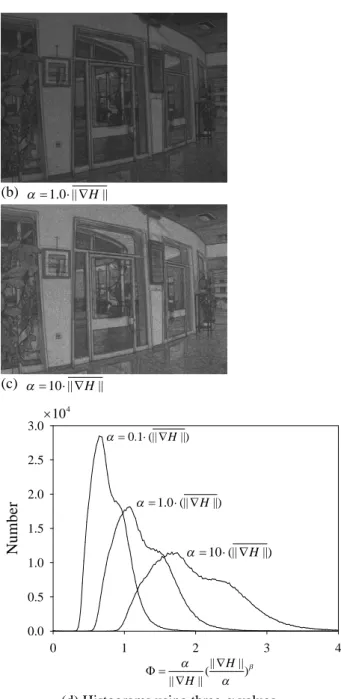
(3) (a). (b) (b) 1.0  || H ||. (c) 10  || H || 10 4. A recommended attenuation function, as in Eqs. (7), is developed by Fattel [3]. This attenuation function suppresses high gradient values more than low gradient values. Two user specified parameters,  and , are used. For  < 0 condition, attenuation function will generate values less than 1. We try to analyzing the effect caused by parameter . In Fig. 3, larger  will induce relative larger attenuated value and cause relative larger variance.  || H ij ||  (7)   ( ) ij. || H ij ||. . 0.1  (|| H ||). 2.5 2.0. Number. Figure 2. The gradient of H. (a) and (b) illustrate the amplitudes of partial differences with x and y components (i.e. H / x and H / y ), respectively. The bottom figure illustrates the gradient magnitude (i.e. || H ij || ). The darker pixels indicate larger values.. 3.0. 1.0  (|| H ||). 1.5. 10  (|| H ||). 1.0 0.5 0.0 0. 1. 2 3  || H ||   ( ) || H || . 4. (d) Histograms using three  values Figure 3. Different  parameters induce variant histograms of the attenuated values. According to Eqs. (7), larger values will induce larger attenuated values and larger variance of attenuated values. As shown in result, too large attenuated values will over emphasize local features. Darker pixels indicate larger attenuated values. The symbol || H || is defined as the mean of magnitudes of gradients. 3.1. Iterations for attenuated luminance. (a) 0.1 || H ||. Once the gradient of H has been attenuated, there should be one corresponding set of luminance to attain the attenuated gradient (G). It is difficult to determine the luminance from one set of known gradient via integration. In order to solve this problem, the attenuated luminance is assumed as orthogonal. The gradient of attenuated luminance ( I ) and attenuated gradient (G) is taken as conservative, and the. - 1105 -.

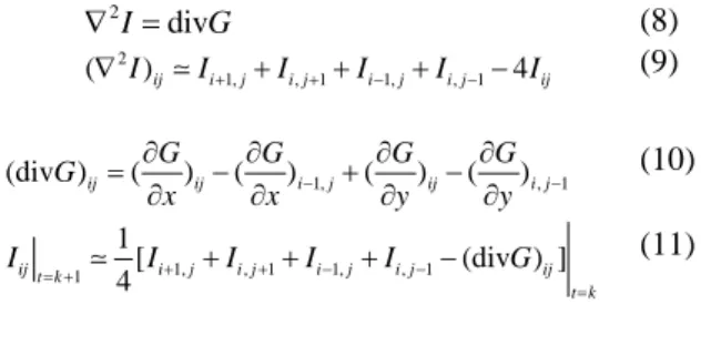
(4) minimization of their surface integration induces Poisson equation, such as Eqs. (8) [3]. The attenuated luminance, which is our objective, will be written as Eqs. (9) according to Laplacian operation. Equation (9) truncates high order term, and these truncated values will be residual or cumulative error. The divergence of the attenuated gradient ( divG ) can be determined by finite difference approximations as in Eqs. (10). We suppose the residual error in Eqs. (9) is small and it can be modified as an iterative form. With given initial values for attenuated luminance ( I ), the iterated-attenuated luminance is solved. The overall procedure of iteration for attenuated luminance is shown in Fig. 4. For convenient purpose, the boundary condition of attenuated luminance ( I ) has zero derivative, for instance I-1,j  I0,j=0. The boundary condition of the attenuated gradient (G) follows the boundary condition of gradient of H. 2 I divG (2 I )ij I i 1, j I i , j 1 I i 1, j I i , j 1 4 I ij (divG )ij ( I ij. t k 1.  G  G  G  G )ij ( )i 1, j ( )ij ( ) i , j 1  x  x  y  y. 1  [ I i 1, j I i , j 1 I i 1, j Ii , j 1 (divG )ij ] 4 t k. conditions as initial values Iinitial. They are constant values, logarithm of initial luminance and simple spatial values. Experimental results are as following. 4.1 Experiment 1: Constant values. We set all initial values 0.5 for iterations. The value is normalized and this specified value is half of the covering luminance. The attenuation function is the typical attenuation gradient, which is Eqs. (7) with 0.1  || H || and = 0.9. As the specified value, all pixels have the luminance ( Iinitial|t=0 ) equals to 0.5. After several iterations, the luminance ( I|t=k ) starts to have values different from 0.5. This is because the luminance propagates especially at high gradient pixels and along the direction of local gradient. Figure 5 illustrates that the constant initial luminance also can be iterated and recover HDR to LDR image via tone mapping.. (8) (9) (10) (11). Via assigning variant kinds of initial values ( Iinitial ), the migrating effect of gradient are revealed. We use three typical conditions for initial values. They are constant values, logarithm of initial luminance and simple spatial values.. (a) t = 20. Let I |t=0 = Iinitial for each pixels ( i, j ) in the image H ij log( I ij ) HDR. for each pixels ( i, j ) in the image { ij functun of ||H ij ||. Gij ij  H ij for each pixels ( i, j ) in the image (divG )ij (. (b) t = 100. }.  G  G  G  G )ij ( )i 1, j ( )ij ( ) i , j 1  x  x  y  y. for ( k=0; k <specified_count; k++ ) for each pixels ( i, j ) in the image 1 I ij  [ I i 1, j I i , j 1 I i 1, j Ii , j 1 (divG )ij ] t k 1 4 t k. (c) t = 100, and recovered with RGB channels Figure 4.. Pseudo-code for progressive iterations.. 4: EXPERIMENTAL RESULTS We have implemented tone mapping operation based one gradient operator. We use Belgium house HDR image for experiments. We take three typical. - 1106 -.

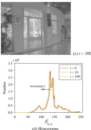
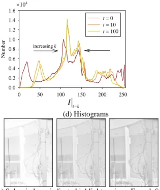
(5) 16 t=0 t=1 t = 20 t = 100. 14. ln(number). 12 10 8 6. increasing k. 4 2. (c) t = 100. 0 0. 50. 100. 150. 200. 250. 3.5. I t k. 10. 4. t=0 t = 10 t = 100. 3.0. (d) Histograms Figure 5. There are 20 and 100 iterations in (a) and (b), respectively. After 100 iterations, a recovered LDR image is shown with coarse grain and flatness patches in (c). The results are shown after many iterations (d).. Number. 2.5 2.0. increasing k. 1.5 1.0. 4.2 Experiment 2: Initial value with logarithmic luminance In this section, we try to focus on speed up the iteration procedure. The initial value of luminance is set to be the same as the logarithmic luminance. Also, the attenuation function is the typical attenuation gradient, which is Eqs. (7) with 0.1   = 0.9. || H || and  Since the value of initial luminance is logarithmic luminance, the attenuated luminance depends on the attenuated gradient. The applied attenuation function is small and has only a little effect on changing the viewing and histogram. Note that the histogram has a tendency to unify distribution of histogram and shift left.. 0.5 0.0 0. 50. 100. 150. 200. 250. I t k (d) Histograms Figure 6. (a) is the original logarithmic luminance. After 10 and 100 iterations (as shown in (b) and (c)), there is only slight change in histogram distribution. 4.3 Experiment 3: Simple spatial global mapping In this section, we use simple spatial global mapping, which was presented by Biswas [1], as the initial luminance ( Iinitial|t=0 ). Also, the typical attenuation function with 0.1  = 0.9 is applied. || H || and  After iterations, the image becomes a little blur, especially in lowlight region. As shown in histogram, more and more extra high and low luminance pixels have been improved. The tendency of histogram is concentrating the central field. The other interesting phenomenon is the improved contrast on highlight region. This is because the extra high luminance effectively migrates to formal luminance.. (a) t = 0. (a) t = 0. (b) t = 10. (c) t = 100. - 1107 -. (b) t = 10.

(6) of its nearest neighbors. It means each pixel only affects its neighbors in one iteration. If we want to propagate the effect of the gradient into a large region, we need lots of iterations. The fact can be seen in the histograms shown in the experiment 1. Hence, the method to design a fast and stable algorithm to avoid the redundancy of computation is an important issue. (3) Initial value and color transfer According to the experimental results (Experiments 1, 2, 3), the different initial values with the same gradients may lead to different experimental results. As shown in experiment 1, the initial value is constant in the beginning, the histograms spread out in when running the iterations. Hence, even if different tone mapping methods are used, methods for achieving and maintaining high contrast and similar color information are important.. 104 1.6 t=0 t = 10 t = 100. 1.4. Number. 1.2 1.0 increasing k. 0.8 0.6 0.4 0.2 0.0 0. 50. 100. 150. 200. 250. I t k (d) Histograms. 5: CONCLUSION. (e) Sub-windows indicate highlight regions. From left to right they are iterated with t=0, t=10 and t=100. 103 3.5 t=0 t = 10 t = 100. 3.0. Number. 2.5 2.0. increasing k. 1.5 1.0 0.5 0.0 160. 180. 200. 220. 240. I t k. (f) Histograms of highlight regions Figure 7. (a) is the original simple spatial luminance. After 10 and 100 iterations (as shown in (b) and (c)), the images become a little blur and dark (as in (d)). The contrast in highlight region has been emphasized (as shown in (e)), and very high luminance is suppressed after iterations. According to the experimental results, some issues are described and discussed in the followings: (1) Attenuation function The purpose of the attenuation function is to compress large magnitude changes (gradient) and preserve local changes of small magnitude as much as possible. However, it is not easy to distinguish the difference between noise and signal. That is to say, noises with local changes of small magnitude may be amplified, and affect the quality of reproduced LDR images. In our nearest future work, we want to deal with the above problem. (2) Iteration and 3*3 local operator In the work of Fattal et al [3], the gradient is approximated using the forward difference among some. Tone mapping is a technique for synthesizing a high dynamic range (HDR) image to a low dynamic range (LDR) image. In this paper, a systematic framework using an attenuation function for tone-mapping is proposed. The way for designing an attenuation function for comfortable scenes is very important in this paper. Two stages for tone-mapping based on gradient operation are proposed. A simple spatial global mapping is firstly used to generate a formal quality LDR image. And then, an adaptive gradient operation is applied for re-enhancing the contrast in high luminance region. In the attenuation function, there are two parameters to be specified. The values of these two parameters depend on the magnitude of gradient of an image. Here, the compromise between quality and efficiency is considered and handled by changing the iterations. Some preliminary results are shown in this paper. In local areas, noise with small gradient magnitude may be amplified and affect the quality of reproduced LDR images. In the future, we want to deal with the above problem.. REFERENCES. [1] K. K.Biswas, S. N. Pattanaik, “ A Simple Spatial Tone Mapping Operator for High Dynamic Range Images,”Proc. IS&T/SID's 13th Color Imaging Conference, 2005. [2] P. E. Debevec and J. Malik, “ Recovering High Dynamic Range Radiance Maps from Photographs,”Proc. ACM SIGGRAPH’ 97, pp. 369-378, 1997. [3] R. Fattal, D. Lischinski, and M. Werman, “ Gradient Domain High Dynamic Range Compression,”ACM Transactions on Graphics, July 2002, pp. 249-256. [4] S. J. Kim and M. Pollefeys, “ Radiometric Self-Alignment of Image Sequences,”Proc. CVPR, 2004. [5] E. Reinhard M. Stark, P. Shirley, and J. Ferwerda, “ Photographic Tone Reproduction for Digital Images,”Proc. SIGGRAPH, 2002. [6] G. Ward Larson, H. Rushmeier, and C. Piatko, “ A Visibility Matching Tone Reproduction Operator for High Dynamic Range Scenes,”IEEE Trans. Visualization and Computer Graphics, 3(4), 1997, pp. 291-306 [7] Ruifeng Xu. Real-Time Realistic Rendering and High Dynamic Range Image Display and Compression. Ph.D. thesis, School of Computer Science, University of Central Florida, Dec, 2005.. - 1108 -.

(7)