利用權重式特徵點比對的車輛周遭監控系統

國

立

交

通

大

學

電機與控制工程學系

碩

士

論

文

利用權重式特徵點比對的車輛周遭監控系統

Vehicle Surrounding Monitoring System using Weighted

Feature Point Matching

研 究 生：方奎理

指導教授：林進燈 教授

利用權重式特徵點比對的車輛周遭監控系統

Vehicle Surrounding Monitoring System using Weighted

Feature Point Matching

研 究 生：方奎理 Student：Kuei-Li Fang

指導教授：林進燈 Advisor：Prof. Chin-Teng Lin

國 立 交 通 大 學

電機與控制工程學系

碩 士 論 文

A Thesis

Submitted to Department of Electrical and Control Engineering College of Electrical Engineering

National Chiao Tung University in Partial Fulfillment of the Requirements

for the Degree of Master in

Electrical and Control Engineering July 2011

Hsinchu, Taiwan, Republic of China

i

利用權重式特徵點比對的車輛周遭監控系統

學生：方奎理

指導教授：林進燈 教授

國立交通大學電機與控制工程學系(研究所)碩士班

摘 要 以研究數字來看，每年的交通事故數量仍然居高不下，其中交通事故中又以車輛與其 他障礙物碰撞事故發生最為頻繁。因此各種提升安全性的高效能車輛與日俱增，諸多研 究人員也提出不同的預防車輛碰撞的安全系統。然而太多的車載系統反而造成使用者在 操作上感到麻煩以及切換不易。因此在本篇論文中，我們提出一個具有整合系統概念的 防碰撞系統，透過四支攝影機來建立車輛周遭影像及整合障礙物偵測技術。為了減低地 面標線對障礙物偵測造成的影響，我們提出一個創新的地面移動量估測技術來降低障礙 物偵測的誤報率。我們手動建立了一個正確的地面移動量表來計算估測誤差藉此來驗證 估測結果。與其他論文的方式做比較，我們所提出的方法提高了地面移動量估測的準確 度並且進一步的減少地面標線所造成的誤報率。本篇論文透過整合兩個系統來減低硬體 成本及使用上的不方便以及提出一個創新的地面移動量估測方式來有效的降低誤報率， 並透過偵測阻礙行進路線上或突出地面具有高度的物體來實現車輛防碰撞警示系統。

ii

Vehicle Surrounding Monitoring System using Weighted Feature Point

Matching

Student:

Kuei-Li

Fang Advisor:

Dr.

Chin-Teng

Lin

Department of Electrical and Control Engineering

National Chiao Tung University

ABSTRACT

The number of traffic accidents is growing up quickly according to the research numbers in every year. Among of all the traffic accidents between vehicle and other generalized obstacles occur most frequently. Therefore, the number of high safety vehicles is increasing over the world. Many researchers proposed various pre-warning collision systems. However, the multi-system will confuse drivers on switching different systems. Hence, this study proposes a pre-warning system and integrates different system. We construct a vehicle surrounding monitoring system through four cameras and integrate an obstacle detection system on the vehicle surrounding monitoring system. In order to decrease the influence caused by ground texture. We also propose a new ground estimation technique to reduce the false alarm rate of obstacle detection. To evaluate the estimation result, we generate a ground truth table by manual to calculate the estimation error. Compared to other paper, our approach promotes the accuracy of ground movement estimation further to reduce the false alarm caused by ground texture. In this thesis, we integrate two systems to decrease the hardware cost and propose a novel ground movement estimation method to reduce the false alarm effectively. By detecting the object significantly arise the road plane, we realize vehicle pre-collision warning system.

iii

致謝

論文的完成，首先要感謝指導教授林進燈教授這兩年來的悉心指導，不管在學業或 生活上都提供我許多意見與想法，這些寶貴的知識讓我受益良多。另外也要感謝張志永 教授、許騰尹教授、蒲鶴章博士等口試委員們的建議與指教，使得本論文更為完整與豐 富。 其次，感謝超視覺實驗室的建霆、子貴、肇廷、Linda、東霖、勝智學長姐們，以 豐富的知識與經驗給予意見及方向，同學們之間的相互砥礪共同奮鬥，共同相處的這段 日子相當愉快，我會懷念我們一起在實驗室相處的時光，還有學弟妹們在研究過程中的 幫忙，提供建議、拍攝影片、打氣鼓勵。其中特別感謝肇廷學長，在理論及程式技巧上 給予我相當多的幫助與建議，讓我獲益良多。還有感謝超視覺實驗室給我的一切，這兩 年來不管是知識的學習還是待人處事上讓我成長很多並且終身受用。 最後要感謝我最愛的父母，對我的教育與栽培，在我求學的路上總是不斷的給予我 鼓勵與關懷，一點一滴，永藏於心，並給予我精神及物質上的一切支援，使我能安心地 致力於學業。 謹以本論文獻給我的家人及所有關心我的師長朋友們。

1

Table of Contents

ABSTRACT in Chinese ... i

ABSTRACT in English ... ii

Chinese Acknowledgements ... iii

Table of Contents ... 1 Chapter 1. Introduction ... 7 1.1. Background ... 7 1.2. Motivation ... 9 1.3. Objective ... 11 1.4. Thesis Organization ... 12

Chapter 2. Related Works ... 13

2.1. Related Work of Vehicle Surrounding Image ... 13

2.2. Related Work of Obstacle Detection ... 17

2.3. System Overview ... 19

Chapter 3. Vehicle Surrounding Image ... 21

3.1. Lens Distortion Correction ... 22

3.1.1. Brief Introduce of Fisheye Lens Distortion ... 22

3.1.2. Distortion Correction Model ... 24

3.2. Image Registration ... 25

3.3. Image Fusion and Lookup Table Generation ... 29

3.3.1. Image Fusion ... 29

3.3.2. Lookup Table ... 30

Chapter 4. Obstacle Detection ... 31

4.1. Feature Point Extraction ... 32

2

4.1.2. Feature Extraction ... 38

4.2. Ground Movement Estimation ... 39

4.2.1. Weighted Feature Point Matching ... 39

4.2.2. Motion Control ... 41

4.3. Obstacle Localization... 41

4.3.1. Image Difference ... 41

4.3.2. Obstacle Localization ... 43

Chapter 5. Experimental Results ... 45

5.1. Experimental Environment ... 45

5.2. Vehicle Surrounding Monitoring ... 46

5.3. Compensation Evaluation ... 50

Chapter 6. Conclusion and Future Work ... 52

3

List of Tables

Table 1- 1: The sub-items of intelligent transportation system ... 7

Table 1- 2: Case number of traffic accidents over the world from 1997 to 2009 ... 9

Table 5- 1 : Camera correction parameter w and image center separately ... 46

Table 5- 2 : Homography matrix of cameras ... 46

4

List of Figures

Fig. 2- 1: The bird eye system in the truck-trailer (a) The kink angle between truck and trailer

is −14° (b) Images capture form omni-directional cameras. ... 13

Fig. 2- 2: (a) A synthetic image consisting of a checkerboard on the ground (b) The back parking result in bird-eye view system ... 14

Fig. 2- 3: (a) Six cameras mounted around the vehicle (b) The sample view of bird-eye view system ... 15

Fig. 2- 4: The bird-eye image of intersection in alley ... 15

Fig. 2- 5: The color corrected vehicle surrounding image ... 16

Fig. 2- 6: Seamless image with smooth illumination ... 16

Fig. 2- 7 : Vehicle surrounding monitoring system flow chart ... 20

Fig. 3- 1: Vehicle surrounding image generation flow chart ... 21

Fig. 3- 2: The rays pass through normal lens ... 22

Fig. 3- 3: The rays pass through fisheye lens ... 22

Fig. 3-4: Barrel distortion in fisheye camera ... 23

Fig. 3- 5: Field of View correction model ... 25

Fig. 3- 6: (a) Original fisheye image and (b) Rectified result. ... 25

Fig. 3- 7: Assumption of virtual camera ... 26

Fig. 3- 8: The reference pattern ... 26

Fig. 3- 9: Projective mapping ... 27

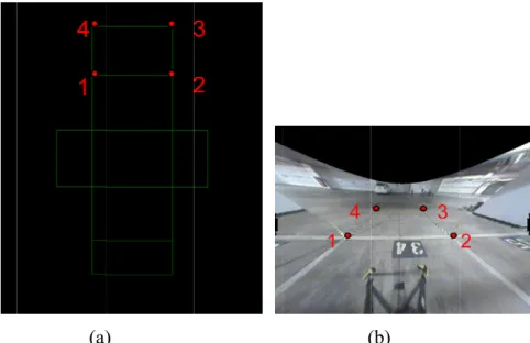
Fig. 3- 10: (a) Reference pattern with four red feature points and (b) Rectified image with four red feature points. ... 28

Fig. 3- 11: Image registration result in single camera image ... 28

Fig. 3- 12: Image registration result in four cameras ... 29

Fig. 3- 13: Overlap seam in vehicle surrounding image ... 30

Fig. 3- 14: Appling pixel weighting function in the vehicle surrounding image ... 30

Fig. 3- 15: Nearest point is chose ... 30

Fig. 4- 1: Obstacle detection system flow chart ... 31

Fig. 4- 2: A color ball i in the L*a*b* color model whose center is at (Lm, *am, *bm) and with radius λmax _{... 35}

Fig. 4- 3 : Sampling area and color ball with a weight which represents the similarity to current road color. ... 36

Fig. 4- 4 : Pixel matched with first B weight color balls which are the most represent standard color. ... 38

5

Fig. 4- 6: The feature point movement ... 39

Fig. 4- 7: The obstacle localization flow chart ... 42

Fig. 4- 8: The difference image between current image and compensated image ... 42

Fig. 4- 9: Radioactive line in the vehicle surrounding image ... 43

Fig. 4- 10: Search every region with a bounding box ... 44

Fig. 5-1 : The system setup environment (a) The front camera is mount on the mark of vehicle (b) In left side and right side, camera is mounted below the rear-view mirror ... 45

Fig. 5-2 : Vehicle surrounding image in driving scene ... 47

Fig. 5- 3 Vehicle surrounding monitoring in driving scene ... 49

Fig. 5- 4: Vehicle surrounding monitoring in parking scene ... 49

7

Chapter 1. Introduction

1.1. Background

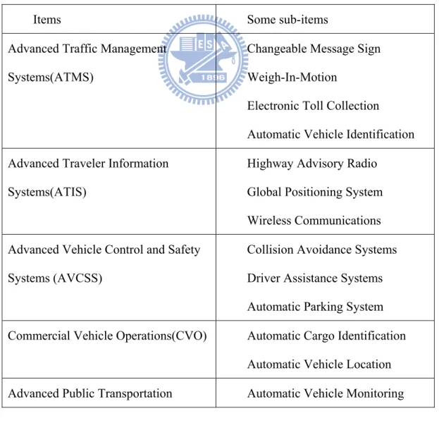
In the 18th century, the vehicle was a simple steam-powered three wheeler. As time goes on, there are many variations on vehicle improvement, such as the change of power, the change of style, and the change of function. Nowadays, consumers no longer only consider vehicle style and vehicle brand, they take different factors into account. Due to the different requirement of consumers, new generation vehicle which involves in the intelligent transportation system (ITS) has been developed rising and flourishing. The intelligent transportation system sub-items are listed in Table 1-1[1].

Table 1- 1: The sub-items of intelligent transportation system

Items Some sub-items

Advanced Traffic Management Systems(ATMS)

Changeable Message Sign Weigh-In-Motion

Electronic Toll Collection Automatic Vehicle Identification Advanced Traveler Information

Systems(ATIS)

Highway Advisory Radio Global Positioning System Wireless Communications Advanced Vehicle Control and Safety

Systems (AVCSS)

Collision Avoidance Systems Driver Assistance Systems Automatic Parking System Commercial Vehicle Operations(CVO) Automatic Cargo Identification

Automatic Vehicle Location Advanced Public Transportation Automatic Vehicle Monitoring

8

Systems(APTS) Electronic Fare Payment

The intelligent transportation system which we emphasize on advanced vehicle can be subdivided into two parts: (1) High performance and pollution-less power (2) Intelligent control and advanced safety.

For high performance and pollution-less power, many engineers have developed some new fuels or power such as bio-alcohol, bio-diesel fuel, hydrogen-based power, and hybrid power. For intelligent control and advanced safety, the goal is to assist drivers when they are inattentive by using sensors and controllers. There are great deals of researches that have been done in this part. For example, pre-collision warning system, intelligent airbags, electronic stability program (ESP), adaptive cruise control (ACC), lane departure warning (LDW) and so on.

In recent year, more and more international vehicle companies or groups have invested in driving safety applications, for example, Toyota, Honda, and Nissan in Japan developed many products continuously. In Europe, the PREVENT project of i2010 will research and promote this project in order to decrease the number of casualty in the traffic accidents.

For driving safety, either vision-based (passive sensor) or radar-based (active sensor) sensing system are used in the intelligent vehicle in order to help driver deal with the situations on the road. The radar-based sensing system can detect the presence of obstacle and its distance, but the drawbacks of this system are low spatial resolution and slow scanning speed. Erroneous judgment will occur when the system is lying in the complicated environment or bad weather. Although vision-based sensing system will also suffer from the environment and weather restriction, it still provide information and real scene to drivers to handle what is happened when the system is alarming.

9

The vision-based sensing system used in the intelligent vehicle can be subdivide into four parts by function: (1) obstacle warning system, (2) parking-assist system, (3) lane departure warning system ,(4) interior monitoring systems [2].

1.2. Motivation

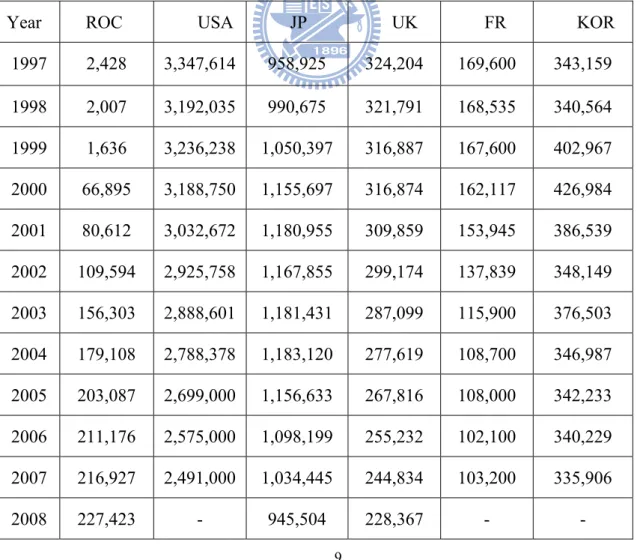
In recent years, the traffic accident number is growing up quickly. According to the statistics [3],[4] in Table 1-2, the number of higher performance vehicles is growing up over the world in recent years, but the number of road traffic accidents number which involves the fatality and injury traffic accidents is still so much. By researching the factors of them, we can refer to a main reason: improper driving, such as inattentive driving, failing to slow down, drunk driver fatigue and so on.

Table 1- 2: Case number of traffic accidents over the world from 1997 to 2009 Year ROC USA JP UK FR KOR

1997 2,428 3,347,614 958,925 324,204 169,600 343,159 1998 2,007 3,192,035 990,675 321,791 168,535 340,564 1999 1,636 3,236,238 1,050,397 316,887 167,600 402,967 2000 66,895 3,188,750 1,155,697 316,874 162,117 426,984 2001 80,612 3,032,672 1,180,955 309,859 153,945 386,539 2002 109,594 2,925,758 1,167,855 299,174 137,839 348,149 2003 156,303 2,888,601 1,181,431 287,099 115,900 376,503 2004 179,108 2,788,378 1,183,120 277,619 108,700 346,987 2005 203,087 2,699,000 1,156,633 267,816 108,000 342,233 2006 211,176 2,575,000 1,098,199 255,232 102,100 340,229 2007 216,927 2,491,000 1,034,445 244,834 103,200 335,906 2008 227,423 - 945,504 228,367 - -

10

2009 180880 - 908,874 208655 - -

To analyze the happening of the accident, we can find that the collision accidents between vehicle and other generalized obstacles occur frequently. (For collision accidents, vehicle could collide with pedestrians, collide with other vehicle, or collide with static objects such as tree or pole.) There is a kind of situation that drivers or passengers alight from vehicle with carelessness. When they open the door directly without checking the nearby objects, they will collide with other pedestrians or motorcyclists or cyclists and then cause accidents. The other one is when we park our vehicle. It is because of the eyesight shelter by the vehicle body, we could not see the region of the other side of vehicle, and our vehicle will probably collided with some objects.

From above statements, we can conclude that it’s necessary and important to acquire the vehicle surrounding scenery to detect the presence of obstacles while driving on the road or parking. And so far, researchers have proposed many methods which focus on the avoidance of collision with front or back coming vehicles. However, too many systems provide different function to avoid collision accidents which is like obstacle warning system, parking-assist system, lane departure warning system, interior monitoring systems. These different systems will confuse driver in switching different system. Besides, in order to mount multisystem in the vehicle for different function will cost a lot of money.

Hence, we propose our research is to provide obstacle detection system based on vehicle surrounding information. That is a vision-based system capable of detecting obstacle in the vehicle surrounding image to integrate the multisystem. We hope that utilize this technology to improve the safety of user when driving the car.

11

1.3. Objective

As mentioned above, the collision accidents between vehicle and other generalized obstacles occur frequently. By developing obstacle detection technique to prevent the car crash is our main purpose. The obstacle which we want to detect is any object that can obstruct the vehicle’s driving path or anything standing significantly from the road surface. Here, many systems are proposed in vehicle safety application. However, too many systems provide different function to avoid collision accidents which is like obstacle warning system, parking-assist system, lane departure warning system, interior monitoring systems. These different systems will confuse driver in switching different system. Besides, in order to mount multisystem in the vehicle for different function will cost a lot of money.

Therefore, the first objective of our research is to develop obstacle detection algorithm based on vehicle surrounding information to integrate multisystem. The other is that to reduce the false alarm rate in obstacle detection. Here, adopting the advantages of vision-based obstacle detector, which have longer and wider detection range relative to radar, and that visual display can make driver to handle the distance of obstacle. We expect to utilize four cameras to achieve vehicle surrounding image to provide image information around the vehicle. Then, to develop obstacle detection system based on the vehicle surrounding information to alarm the driver. By proposing the vehicle surrounding monitoring system, we want to prevent some car crashes and to improve the safety.

12

1.4. Thesis

Organization

The remainder of this thesis is organized as follows. Chapter 2 describes related works about vehicle surrounding image and obstacle detection. Chapter 3 shows vehicle surrounding image generation. Chapter 4 introduces obstacle detection algorithm including feature point extraction, ground movement estimation, and obstacle localization. Chapter 5 demonstrates experimental results and evaluations. Finally, conclusions and future works are presented in chapter 6.

13

Chapter 2. Related Works

Many researchers make efforts in vehicle surrounding monitoring and obstacle detection. They propose many different systems in collision pre-warning system. In this chapter we will briefly describe these papers and its technique. We will subdivide related work to two parts. One is vehicle surrounding monitoring system and the other is obstacle detection.

2.1. Related Work of Vehicle Surrounding Image

Ehlgen and Pajdla [5] proposed a system, which generates a bird-view of the surrounding area of a truck-trailer. This system consists of four omni-directional cameras mounted on a truck. Here, they use a magnetic sensor to measure the angle between the truck and trailer. By using the information captured by magnetic sensor to stitch images into a correct bird-view image, which is shown in Fig. 2.1.

(a) (b)

Fig. 2- 1: The bird eye system in the truck-trailer (a) The kink angle between truck and trailer is −14° (b) Images capture form omni-directional cameras.

Ehlgen et al. [6] proposed a backing up system based on two catadioptric cameras. They mounted two catadioptric cameras on a vehicle and provided the driver with a bird-view of the surrounding area behind the vehicle as well as the area on the left and right hand side. To enlarge the field of view of the bird-view image, an extension assumption to the bird-view image is used that provides a larger field of view, which is shown in Fig.2-2.

14

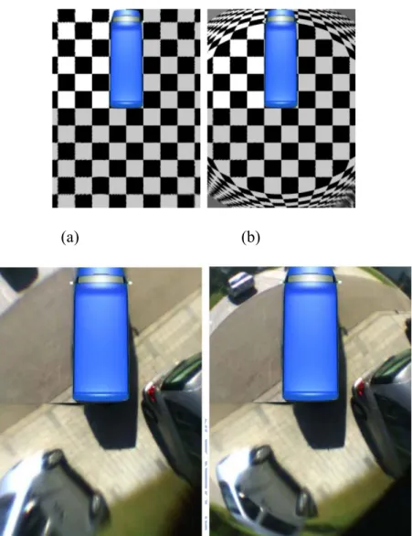
(a) (b)

Fig. 2- 2: (a) A synthetic image consisting of a checkerboard on the ground (b) The back parking result in bird-eye view system

Liu et al. [7] proposed a vehicle surrounding system based on six fisheye cameras mounted around a vehicle, shown in Fig.2-3. Due to many cameras used, the views of their system cover whole surrounding area. This system uses a flat plane to stitch six fisheye camera’s image, and this system divide each fisheye camera’s display area according to the optimal seams, which are decided by the distribution of each fisheye camera’s calibration error, which is shown in Fig. 2-3.

15

Fig. 2- 3: (a) Six cameras mounted around the vehicle (b) The sample view of bird-eye view system

Liu et al. [8] proposed a vehicle surrounding monitoring system based on embedded system. The researcher utilizes the four cameras to generate bird-eye view image and ports their system on the DSP embedded system. They use a dynamic boundary method to deal with the ghost problem on two different image covered regions, which is shown in Fig. 2-4.

Fig. 2- 4: The bird-eye image of intersection in alley

Y.-F. Chen et al. [9] proposed a parking assistant system based on four cameras to build vehicle surrounding image. This system uses a reference pattern to correct the camera and applies a simple statistic method to achieve color consistency, the result which is shown in Fig. 2-5.

16

Fig. 2- 5: The color corrected vehicle surrounding image

C. L. Ho et al. [10] proposed a system with image refinement to generate surrounding image. They compensate vignetting effect and uniform illumination to optimize the surrounding image. By blending the color of the overlapped region, they can obtain the seamless images with smooth illumination, which is shown in Fig. 2-6.

17

2.2. Related Work of Obstacle Detection

The obstacle detection is the primary task for intelligent vehicle on the road, since the obstacle on the road can be approximately discriminated from pedestrian, vehicle, and other general obstacles such as trees, street lights and so on. The general obstacle could be defined as objects that obstruct the path or anything located on the road surface with significant height.

Depending on the number of sensors being used, there are two common approaches to obstacle detection by means of image processing: those that use a single camera for detection (monocular vision-based detection) and those that use two (or more) cameras for detection (stereo vision-based detection).

The stereo vision-based approach utilizes well known techniques for directly obtaining 3D depth information for objects seen by two or more video cameras from different viewpoints. Koller et al. [11] utilized disparities in correspondence to the obstacles to detect obstacle and used Kalman filter to track obstacles. A method for pedestrian(obstacle) detection is presented in [12] whereby a system containing two stationary cameras. Obstacles are detected by eliminating the ground surface by transformation and matching the ground pixels in the images obtained from both cameras. The stereo vision-based approaches have the advantage of directly estimating the 3D coordinates of an image feature, this feature being anything from a point to a complex structure. The difference in viewpoint position causes a relative displacement, called disparity, of the corresponding features in the stereo images. The search for correspondences is a difficult, time-consuming task that is not free from the possibility of errors. Therefore, the performance of stereo methods depends on the accuracy of identification of correspondences in the two images. In other words, searching the homogeneous points pair in some area is the prime task of stereo methods.

18

The monocular vision-based approaches utilize techniques such as optical flow. For optical flow based methods which indirectly compute the velocity field and detect obstacle by analyzing the difference between the expected and real velocity fields, Kruger et al. [13] combined optical flow with odometry data to detect obstacles. However, optical flow based methods have drawback of high computational complexity and fail when the relative velocity between obstacles and detector are too small. Inverse perspective mapping (IPM), which is based on the assumption of moving on a flat road, has also been applied to obstacle detection in many literatures. Ma et al. [14][15][16] present an automatic pedestrian detection algorithm based on IPM for self-guided vehicles. To remove the perspective effect by applying the acquisition parameters (camera position, orientation, focal length) on the assumption of a flat road geometry, and predicts new frames assuming that all image points lie on the road and that the distorted zones of the image correspond to obstacles. Bertozzi et al. [17] develop a temporal IPM approach, by means of inertial sensors to know the speed and yaw of the vision system and the assumption of flat road. A temporal stereo match technique has been developed to detect obstacles in moving situation. Although these methods could utilize the property of IPM to obtain effective results, but all of these should rely on external sensors such as odometer or inertial sensor to acquire ego-vehicle’s displacement on the ground that enables them to compensate movement over time for the ground plane. Yang et al. [18] proposed a monocular vision-based approach by compensating for the ground movement between consecutive top-view images using the estimated ground-movement information and computes the difference image between the previous compensated top-view image and the current top-view image to find the obstacle regions. J.C. Lee et al [19] proposed a monocular vision-based approach by compensating for ground movement. They proposed a new feature point extraction method to support ground movement estimation effectively. To use road detection on the feature point extraction, they can separate feature point which is on the

19

obstacle. By on-line training the road color model, the feature points can be ensured on the ground plane.

2.3. System

Overview

The overall system flowchart is shown in Fig. 2-7. At the beginning, we will utilize the FOV fisheye correction model to deal with lens distortion effect in wide angle camera, and yield a non-distorted image. In the next step, we assign the corner point by manual and draw the reference pattern to calculate a appropriate homography matrix. By using the homography matrix we transform our original image into bird-view image. Then, we apply pixel weighting function to calculate the weighting of each image in the image cover region to achieve the seamless surrounding image. Finally, we build up a lookup table to realize a vehicle surrounding monitoring image, and the detailed contents will be described in Section 3.

While we generate the vehicle surrounding image, we exploit road detection algorithm to distinguish the road and non-road in order to support the feature point extraction. Due to the characteristic of road color, we transform the RGB images into Lab color space to effectively distinguish road and non-road, the procedure will be introduced in Section 4-1. The next step, we analysis the features which are suitable for track in our condition, the road color similarity and the features which gradient is satisfied the restriction in the road region is selected. As we obtain feature points in vehicle surrounding image coordinate, the principal distribution of ground movement will be estimated by the proposed method WFPM. By estimating ground moving value, we build a compensated image which is shifted by the estimated ground movement. Finally, we detect obstacle by the difference between current image and compensated image and the nearest position to vehicle will be located. The obstacle detection procedure will be shown in Section 4 in detail.

20

21

Chapter 3. Vehicle Surrounding Image

In this chapter, we are going to introduce the generation of the vehicle surrounding image. At first, we will introduce how we correct the lens distortion effect in the fisheye camera, and yield undistorted image. Once we generate the undistorted image, we utilize the homography matrix to transform the undistorted image into the bird-view image. By using the weighting function, we can eliminate the seam in the stitching image. Finally, we make up a lookup table to achieve vehicle surrounding image. The following Fig.3-1 is the flow chart of vehicle surrounding image generation.

22

3.1. Lens Distortion Correction

3.1.1. Brief Introduce of Fisheye Lens Distortion

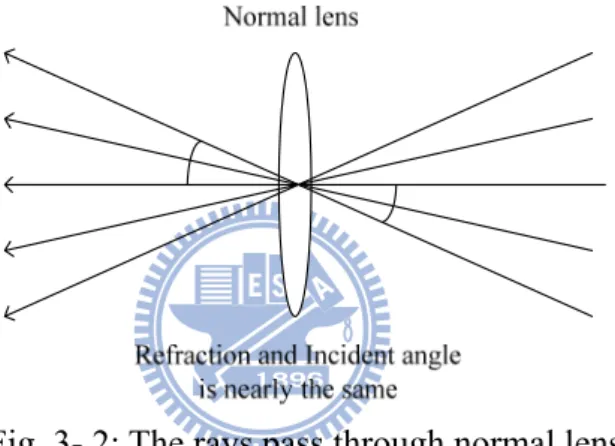
In order to capture wide angle image, we utilize the fisheye camera mounted around a vehicle. However, in the wide angle camera, lines will deform because of the fisheye lens distortion effect. We want to remove the distortion to be convenient on image registration. First, we discuss on lens distortion effect generation. Normal lens with natural field of view does not subject to perspective distortion. The refraction angle of the image and the incident angle is nearly the same, as shown in Fig. 3-.

Fig. 3- 2: The rays pass through normal lens

As shown in Fig. 3-3, we can observe that the refraction angle of the image is smaller than the incident angle. Thus a fisheye lens with wider field of view always subject to more serious perspective distortion, for example, barrel distortion as illustrated in Fig. 3-4.

23

Fig. 3-4: Barrel distortion in fisheye camera

In general, lens correction can be classified into two basic methods [20] [21]: (1) The polynomial and curve fitting based method (parametric based), (2) The model and optimization based method (non-parametric based).

In the polynomial and curve fitting based method, the images often be corrected by using the nonlinear optimization of the points lying on some 3D objects or planar grids. As the distortion effect is significant, it will cost more time and increase heavier computational complexity to estimate the distortion coefficients. In another method, the model and optimization based method, it is due to the polynomial methods which do not perform well for serious distortion image. According to the best parameter values obtained by the feature optimization, it can handle higher precision in significant distortion effect. The following are these two methods mentioned above.

Polynomial Distortion Model

In polynomial distortion model, the lens distortion model can be written as an infinite series.

x x 1 κ κ y y 1 κ κ

Where the κ , κ is the radial symmetric distortion parameter ,and the r is the distorted radius means the distance form distorted pixel to image center. By find out the higher order terms parameter in the function, the distortion effect can be corrected exactly.

24

The Field of View distortion model was based on the principle common formation of fisheye lens which has only one parameter. The r is the mentioned above and the ω is the field of view of the corresponding fisheye lens.

r 1 ωtan 2r tan ω 2 r tan r ω 2 tanω₂ r x y , r x y

In the model, the radial constraint and the only one parameter of the fisheye lens are adequately used to handle the lens radial distortion.

3.1.2. Distortion Correction Model

In this thesis, we utilize the Field of View correction model mentioned in [20] to rectify the distortion line into the straight line. We assume the object point P in the world coordinate, it project on the image plane m, and the undistorted projection point m, which is shown in Fig.3-5. The relation between p and p can be described by the formula. Where x is the horizontal distance between image center to the pixel p and y is the vertical distance between image center to the pixel p . Where x is the distance frame image center to the virtual undistorted pixel p. Where r is the undistorted radius and the r is the distorted radius. According to the FOV model, the lens distortion can be fitted excellently in the field of view distortion model by finding the w parameter. In Fig. 3-6, we demonstrate the original distort image and the rectified result.

3.2

woul the p

. Ima

While we c ld remain st perspective e F (a) Fig. 3- 6: (

age Reg

calibrate the traight in th effect and y Fig. 3- 5: Fi r r x (a) Original

gistratio

e image cap he virtual im yield a virtu 25 ield of View 1 wtan 2 r tan 2 ta x y , r l fisheye im

on

ptured by th mage. Next, ual bird view

w correction 2r tanw 2 r w an w₂ r x mage and (b) he wide ang the target o w image. n model y (b) ) Rectified r gle camera, of image re result. all of the s gistration is straight line s to remove e e

coord it can draw and trans whic mapp In the gene dinate plane n capture b wn as follow The next st four rectif sformation ch is shown ping, which eration of b e and the vi ird view im wing, shown tep, we hop fied image is a projec n in Fig.3-9 h is shown in bird view im irtual camer mage around n in Fig.3-7. Fig. 3- 7: A Fig. 3-pe to find th s to build tion from a 9. The gene n. Eq. (3-1) 26 mage, we as ra mounted d the vehicl Assumption 8: The refe he homogra d the bird a plane to eral form o ) ssume the g on the top o le. Here, the

of virtual c erence patte aphy transfo view imag another pl of a project ground plan of the car. F e virtual bir camera ern orm between ge. Perspec ane through tive mappin e on the Z= For this virtu

rd view pat n the refere ctive or h h the refer ng is a rati =0 of world ual camera, ttern can be ence pattern homography ence point, ional linear d , e n y , r

and d homo verti can b in the pixel imag The p Projective m destination ography ma ces number be found by To implem e virtual ref l: 2.5 cm).W ges and in vi process of t mapping ha coordinates atrix we use red cyclicall y solving the u v u v u v u v 0 0 0 0 0 0 0 0 ment that we ference patt We mark out irtual image this procedu Fig. 3 x au b gu x y w as 8 degrees s of the four e in [22]. Le ly k=0, 1, 2 e 8*8 linear 1 0 0 1 0 0 1 0 0 1 0 0 0 u v 0 u v 0 u v 0 u v assign the tern. The vir

t the corresp es by manua ure can be s 27 - 9: Project bv c hv i , p a b d g h s of freedom r corners of et the corres , 3. Assume r equation, w 0 u x 0 u x 0 u x 0 u x 1 u y 1 u y 1 u y 1 u y correspondi rtual referen ponding fou al to calcula how on Fig tive mappin y du e gu h M p b c e f h i uv q m which can a quadrilate sponding ma e that i=1 , t which is sho x v x x v x x v x x v x y v y y v y y v y y v y ing feature nce pattern ur feature po ate homogra g 3-10 and F g ev f hv i u v q n be determi eral. The ca ap u , v T the eight pa own in Eq. ( a b c d e f g h = points in th is drew in a oints separa aphy transfo Fig.3-11. ined from th alculation of to x , y arameter in t (3-2). x x x x y y y y he calibrated a proportion ately in rect ormation m (3-1) he source f the T _for the matrix (3-2) d image and nal scale (1 ified matrixes. d

Fig. patte 3- 10: (a) R After we ca ern to genera (a) Reference pa Fig. 3- 11 alculate the ate bird view

) attern with f r : Image reg homograph w image. T 28 four red fea red feature gistration re hy matrix, a he result is ( ature points points. sult in singl all the image

shown in F (b) and (b) Rec le camera im es can be as Fig 3-12 ctified imag mage ssigned to th ge with four he virtual r

29

Fig. 3- 12: Image registration result in four cameras

3.3. Image Fusion and Lookup Table Generation

3.3.1. Image Fusion

In image fusion, we deal with the image stitching result. For image stitching, the remarkable illumination difference between two source images, an obviously seam will appear after the stitching process. In Fig.3-13 shows boundary seam caused by illumination different. Here, we apply the pixel weighting function to handle the effect. Supposed two overlapped region in the target image I , and reference image I is respectively A and B, Where A x, y I , B x, y I . The fusion image is I, and then we can obtain equation (3.3)

I x, y I , x, y I A 1 r B r , x, y I I I , x, y I A I , B I (3.3) Among Eq. (3.16), r expresses the weight value, which is determined by overlapped region width d, and the range of r is 1→0 which increases based on r. We can know when r changes slowly from 1 to 0, then the image will slowly smooth translation from I to I , therefore eliminates illumination boundary. In Fig. 3-14, we show the image fusion result of Fig. 3-13.

3.3.

looku apply interp hole, appro Fig. 3-

.2. Look

In order to up table, ev y this techn polate black , we can fin oach to inte Fig. 3- 14: Appling

kup Tab

o reduce the very pixel w nique, there k hole with nd the posit erpolate the 13: Overlap g pixel weig

ble

e calculatin will assigns is some bl a pixel valu tion of orig black hole, Fig. 3- 30 p seam in ve ghting funct ng time, we appropriate ack hole in ue. By appl ginal image. shown in F 15: Nearest ehicle surro ion in the v e generate a e position to n the buildin lying the inv

Then, we Fig. 3-15. point is cho ounding ima vehicle surro a lookup ta o build the ng image. A verse transf utilize the n ose age ounding ima able. Accor final image As a result, formation fo nearest neig age ding to the e. While we we have to or the black ghbor point e e o k t

31

Chapter 4. Obstacle Detection

In this chapter, we describe the obstacle detection which applies on the vehicle sounding image. First of all, we extract appropriate feature points by combining road detection to ensure these points which are on the road. And, in order to reduce the false alarm caused by ground texture, we assume that the ground texture movement is same to ground movement. According to selected feature points mentioned above, we propose ground movement estimation method WFPM to estimate the movement of ground. By the estimated movement, we construct a compensated image to model the ground texture movement in driving. The obstacle will be detected by the difference of vehicle surrounding image and compensated image. Finally, we locate the obstacle by searching radioactive line around the car center to alarm the driver. The flow chart of the obstacle detection is shown Fig. 4-1.

32

4.1. Feature Point Extraction

Feature points are used to estimate ground movement by its corresponding relationship between one frame and subsequent frame. Considering the objective, to select an appropriate point is important for us. If we choose a point on a large blank wall then it won’t be easy to find that same point in the next frame of a video. If all points on the wall are identical or even very similar, then we won’t have much luck tracking that point in subsequent frames. On the other hand, if we find a point that is unique then we have a pretty good chance of finding that point again.

In practice, the point or feature we select should be unique, or nearly unique. It should be parameterizable and it can be compared to other points in another image. As a result, we might be tempted to look for points that have some significant change within neighboring local area. We say that is the good features which have a strong derivative in spatial domain. Another characteristic of features is about the position of the image.

Considering that the objective of the following procedure is to estimate the ground movement information. Features lie on the ground region is useful criteria for the following ground movement estimation algorithm. Due to above analysis, a good feature to track should have two characteristics. First, a feature should have strong derivative which could assist us to track them and obtain a precise motion. Then, the position of feature should be restricted on the road region (non-obstacle region). The features which we will use them to estimate the ground movement information should conform the above two characteristic, these features will be suitable for estimating ground movement information.

We proposed a feature point extraction method employ road detection procedure to support in getting ground features.

To utilize the result of the road detection, major road color is compared to the feature point’s color to ensure these good features within road region. By integrating road detection, the more

33

useful ground features could be extracted and could improve results of ground movement effectively. The next chapter 4.1.2 will introduce the detail of road detection and describe what feature point will be selected.

4.1.1. Road Detection

The proposed feature point extraction technique is integrating a road detection procedure [23]. This procedure uses an on-line color model that we can train an adaptive color model to fit road color. The main objective of road detection is to discriminate the road and non-road region roughly, because the result is used to support feature extraction not used to extract obstacle regions. However, we adopt an on-line learning model that allows continuously update during driving, through the training method that can enhance plasticity and ensure the feature is on the road region.

Due to the color appearance in the driving environment, we have to select the color features and using these color features to build a color model of the road. Therefore, we have to choose a color space which has uniform, little correlation, concentrated properties in order to increase the accuracy of the model. In computer color vision, all visible colors are represented by vectors in a three-dimensional color space. Among all the common color spaces, RGB color space is the most common color feature selected because it is the initial format of the captured image without any distortion. However, the RGB color feature is high correlative, and the similar colors spread extensively in the color space. As a result, it is difficult to evaluate the similarity of two color from their 1-norm or Euclidean distance in the color space.

The other standard color space HSV is supposed to be closer to the way of human color perception. Both HSV and L*a*b* resist to the interference of illumination variation such as the shadow when modeling the road area. However, the performance of HSV model is not as good as L*a*b* model because the road color cause the HSV model not uniform that lead to

34

the HSV color model not as uniform as the L*a*b* color model. There are many reasons attribute this result. Firstly, HSV is very sensitive and unstable when lightness is low. Furthermore, the Hue is computed by dividing (Imax - Imin) in which Imax = max(R,G,B), Imin =

min(R,G,B), therefore when a pixel has a similar value of Red, Green and Blue components, the Hue of the pixel may be undetermined. Unfortunately, most of the road surface is in similar gray colors with very close R, G, and B values. If using HSV color space to build road color model, the sensitive variation and fluctuation of Hue will generate inconsistent road colors and decrease the accuracy and effectiveness. L*a*b* color space is based on data-driven human perception research that assumes the human visual system owing to its uniform, little correlation, concentrate characteristics are ideally developed for processing natural scenes and is popular for color-processed rendering. L*a*b* color space also possesses these characteristics to satisfy our requirement. It maps similar colors to the reference color with about the same differences by Euclidean distances measure and demonstrates more concentrated color distribution than others. Then considering the advantaged properties of L*a*b* for general road environment, the L*a*b* color space for road detection is adopted.

The RGB-L*a*b* conversion is described as follow equations: 1. RGB-XYZ conversion: 0.431 0.342 0.178 X = ⋅ +R ⋅ +G ⋅ B 0.222 R+0.707 G+0.071 B Y = ⋅ ⋅ ⋅ 0.020 0.130 0.939 Z = ⋅ +R ⋅ +G ⋅ B 2. Cube-root transformation:

35 1 3 1 3 * 166 16 >0.008856 * 903.3 0.008856 * 500 [ ( ) ( )] * 200 [ ( ) ( )] X , , , XYZ n n n n n n n n n n n Y Y L if Y Y Y Y L if Y Y X Y a f f X Y Y Z b f f Y Z

where Y Z are tristimulus values of reference white poi

⎧ _{⎛ ⎞} ⎪ _{= ⋅⎜ ⎟ −} ⎪⎪ ⎝ ⎠ ⎨ ⎪ _{⎛ ⎞} ⎪ = ⋅_{⎜ ⎟} ≤ ⎪ _{⎝ ⎠} ⎩ = ⋅ − = ⋅ − 1 3 _>0.008856 ( ) 7.787 16 /116 0.008856 n n n n n nt X = 95.05,Y = 100,Z = 108.88 Y t Y f x Y t Y ⎧ ⎪ ⎪ = ⎨ ⎪ _{+ ≤} ⎪⎩

By modeling and updating of the L*a*b* color model, the built road color model can be used to extract the road region. The L*a*b* model is constituted of K color balls, and each color ball mi is formed by a center on (Lmi,*ami,*bmi) and a fixed radiusλmax =5 as seen in

Fig. 4-2.

Fig. 4- 2: A color ball i in the L*a*b* color model whose center is at (Lm, *am, *bm) and with radius λmax

36

In order to train a color model, we set a fixed area around the car in the vehicle surrounding image by manual and assume pixels in this area are the road samples. In the beginning few frames are used to initialize the color model for each pixel in the sample region. And update the model every fixed frame to increase processing speed but still maintain high accurate performance.

The sampling area is used to be modeled by a group of K weighted color balls. We denote the weight and the counter of the mi th color ball at a time instant t by Wm ti, and

,

i

m t

Counter _{, and the weight of each color ball represents the stability of the color. The color}

ball which more on-line samples belonged to over time accumulated a bigger weight value shown in Fig. 4-3. Adopting the weight module increases robustness of the model.

Fig. 4- 3 : Sampling area and color ball with a weight which represents the similarity to current road color.

The weight of each color ball is updated by its counter when the new sample is coming which is called one iteration. Therefore, the counter would be initialized to zero at the beginning of iteration. The counter of each color ball records the number of pixels added from

37

the on-line samples in the iteration. The first thing to do is that which color ball is chosen to be added. We measure the similarity between new pixel xt and the existing K color balls using a Euclidean distance measure (4-1). The maximum value of K is also set to limit the color ball number. 2 2 2 max ( , ) ( ) ( ) ( ) i i i i m x m x m x Similarity x m =sqrt_⎣⎡ L −L + a −a + b −b ⎤_⎦<=λ (4-1) If a new pixel xt was covered by any of the color ball in the model, one will be added to the counter of best matching color at this iteration as the equation (4-2). After entire new sample pixels at this iteration undertake the matching procedures mentioned above, the weights of every color ball are updated according to their current counter and their weight at last iteration. The updating method is as follows:

i i m i i max m(x ) = arg min(Similarity(x ,m ) <=λ ) (4-2) , 1 (1 ) / [0,1], i i m t w t w m sample w sample W W counter N N α α α + = ⋅ + − ⋅ ∈

, where αwis user-defined learning rate, N sample is the sampling area

Then using the weight to decide which color ball of the model most adapt and resemble current road. The color balls are sorted in a decreasing order according to their weights. As a result, the most probable road color features are at the top of the list. The first B color balls are selected to be enabled as standard color for road detection, and these color balls with a higher weight has more importance in detection step. Road detection is achieved via comparison of the new pixel xt with the existing B standard color balls selected at the previous instant of time shown in Fig. 4-4. If no match is found, the pixel xt is considered as non-road. On the contrary, the pixel xt is detected as road.

38

Fig. 4- 4 : Pixel matched with first B weight color balls which are the most represent standard color.

4.1.2. Feature Extraction

As mentioned above, we consider two characteristics which are strong derivative and ground feature. The road region and strong gradient points are selected to be feature points. Therefore, the first criterion of feature point extraction is to extract the major strong gradient points using Sobel edge detector. For each extracted feature points, we compare its color information to the road color model to distinguish the feature points on road or on the obstacle. And the nearest position constraint is considered together to enhance the selection. Then the feature points are collected completely by these road boundary and high gradient features. In Fig. 4-5 shows the result of feature point extraction. By employing road detection to support feature point extraction, the more useful ground features can be extracted.

39

4.2. Ground Movement Estimation

Considering the road texture on the ground will cause false alarm rate of obstacle detection system. Assume that the ground texture movement attached on ground is same to the ground movement. Hence, we propose a WFPM method to estimate the ground movement vector. By compensating the ground plane movement with estimated vector we can reduce the false alarm caused by road texture. The following will brief describe the estimation method WFPM.

4.2.1. Weighted Feature Point Matching

Our estimation method WFPM (Weighted Feature Point Matching) is similar to FPM (Feature Point Matching) algorithm [24] to calculate the ground movement. The FPM technique is proposed to solve the digital image stabilization. Here, the original equation of FPM is shown in Fig. 4-6. The correlation calculation of FPM is by

, | 1, , , , |

Fig. 4- 6: The feature point movement

The N is the total number of feature point, I(t-1,x,y) is the intensity of the representative point (x , y) at frame t-1 , and , is the correlation measure for a shift (p , q) between the representative points in image at frame t-1 and the relative shifting points at frame t. Assuming , is the minimum correlation value in image,

40

, _, , , the ground movement vector v that produces the minimum correlation value, , , , , .

We propose a new method called Weighted Feature Point Matching method which is based on the FPM technique to estimate the ground movement. Here, the road detection information will be used to enhance the matching correctness effectively. As mentioned above, the feature point extraction in section 4.1, we utilize the road color model to distinguish the feature points on road or not. We set up a fixed threshold to reselect the feature points. However, these feature points which exceed the threshold still be different for the similarity of road color. Due to this reason, the feature point more similar to the road color, the more reliability should be assign to the feature point. In here, for every pixel exceeds the threshold, we give a road reliable weight in following criterion.

Quantitative criterion:

# .

_

Also we think about reliability on the feature points exceed the intensity threshold. If the intensity higher, the more reliability weight should be assign to feature point. The following is the intensity reliable weight criterion.

Quantitative criterion:

# .

_

We apply the road reliable weight and intensity reliable weight on the feature point matching method to enhance the matching. Therefore, the FPM correlation calculation equation rewrite to the following equation:

_ _∑ _

41

_{_} _

∑ _{_} , _ 1

, 1, , , , _{_ _}

4.2.2. Motion Control

By considering the temporal constraint, the scene will not change a lot during the few frames. For these reason, value of ground movement vector is anomalous relative to the neighboring frames would indicate the compensation information is not correct.

Through observing the recent frames can assist us to ensure the ground movement information is correct or not. Because the correctness of ground movement is greatly determining the results of following detection procedure, the verification is essential and worth to undertake. If the equation is conformed, that is indicating anomalous amount of obstacle candidate and the ground movement information in the current frame possibly erroneous. Then the previous compensation information will be utilized to compensate.

Quantitative criterion:

.

(4-6) Where Thd. is user-defined threshold

By applying the motion control technique, we can reduce the error of estimation information and validate the compensation information more reliable.

4.3. Obstacle Localization

4.3.1. Image Difference

The obstacle residue map can be obtained by the difference between current image and the compensated image, shown in Fig.4-7. It can be determined whether a point is on the ground

plane (see corre imag indic diffe are d e or not by Eq. 4-7), w esponding p ge differenc cate every p rence betw determined a Inpu Imag Compen Imag | _ Fig. 4- 8 comparing where △ is points. In th ce is compl pixel is bel een current as obstacle. ut ge nsated ge Fig 8: The differ g the gray v s the thresh his way, w leted, the o longing to o t image and Diffe g. 4- 7: The _ rence image 42 values of the hold for the we can detec obstacle can obstacle or d compensat erence Obstacle L obstacle lo | e between c e correspon e maximum ct obstacles ndidate ima not. Fig. 4 ted image, Obs Locali Localiztion calization f urrent imag nding pixels m disparity s above the age is obtai 4-8 shows s the pixels w stacle ization flow chart , , ge and comp s on two im of gray va e ground pl ined which some result while the co pensated im mage frames alue of two lane. When is used to ts of image olor is blue (4-7) mage s o n o e e

43

4.3.2. Obstacle Localization

The special characteristic of the obstacle are used to detect obstacle in bird view coordinate, shown in Fig.4-9. The object significantly stand on the ground plane will appear radioactive line in the bird view image.

Fig. 4- 9: Radioactive line in the vehicle surrounding image

To utilize the characteristic in obstacle, we divide the image every four degree as a scan region. By moving a bounding box in this region, we can add up the radioactive line number in each region. If the radioactive line numbers in the bounding box are over the threshold we set, we locate the lowest position of the radioactive line as the obstacle to vehicle, shown in Fig.4-10.

44

Fig. 4- 10: Search every region with a bounding box

Finally, we use the proportional scale (1 pixel: 2.5 cm) which is mentioned in section 3-2 to calculate the real distance in world coordinate. Here, the distance between vehicle and obstacle will be separated in different emergency color. The red color label means the obstacle nears vehicle less than two meters. The yellow color label means the obstacle nears vehicle between two meters to four meters. The green color label means the obstacle nears vehicle longer four meters.

45

Chapter 5. Experimental Results

In this chapter we will demonstrate our research results. The experimental environment will be introduced at first. Next, we will separately demonstrate the vehicle surrounding image and its detection result. In compensation evaluation, we will generate a ground truth to evaluate proposed method.

5.1. Experimental

Environment

The environmental vehicle is Mitsubishi Savrin. The four wide angle cameras is setup separately around the vehicle, shown in Fig.5-1.

(a)

(b)

Fig. 5-1 : The system setup environment (a) The front camera is mount on the mark of vehicle (b) In left side and right side, camera is mounted below the rear-view mirror

46

Our algorithm is implemented on the platform of PC with Intel Core2 Duo 2.2GHz and 2GB RAM. Borland C++ Builder is our developing tool and operated on Windows XP. All of our testing inputs are uncompressed AVI video files. The resolution of video frame is 320*240.

5.2. Vehicle Surrounding Monitoring

Lens distortion correction parameters of four cameras are shown in Table 5-1. The corresponding homography matrix of cameras is shown separately in Table 5-2.

Table 5- 1 : Camera correction parameter w and image center separately Camera W Image Center

Front 0.0056 160 98 Back 0.00558 160 92

Left 0.00565 163 98 Right 0.00569 158 98

Table 5- 2 : Homography matrix of cameras

Front Back 0.119 0.702 125.23 -1.227 4.905 2175.25 0.002 0.402 71.17 0.204 6.27 2387.83 7.074 0.003 0.435 0.0002 0.0255 9.0298 Left Right 3.047 -0.01 -505.4 -1.088 -0.161 607.8 2.2967 0.72894 -459.69 0.9595 0.335 96.00 0.01531 -0.0010 -1.375 -0.0063 0.0006 2.851

47

The following is the vehicle surrounding image without obstacle function in driving scene which is shown in Fig. 5-2.

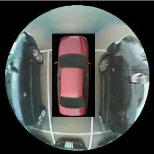
Fig. 5-2 : Vehicle surrounding image in driving scene

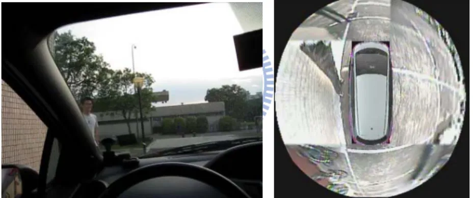
By applying the obstacle detection on the vehicle surrounding image, we detect the obstacle when user driving and parking to prevent collision accident. Fig. 5-3 and Fig. 5-4 demonstrate the experimental results of obstacle detection in vehicle surrounding image for various conditions.

49

Fig. 5- 3 Vehicle surrounding monitoring in driving scene

50

5.3.

Compensation Evaluation

In order to verify the accuracy of proposed ground movement estimation technique, an

experiment is designed to evaluate compensation of ground movement. At first, we have to establish ground truth manually that can assist us to evaluate the estimation results. Considering that we are going to evaluate the compensation of ground movement, we pick up three ground points for each frame and corresponding positions in previous frame. As shown in Fig. 5-5, the three ground points marked between consecutive frame images.

Previous frame Current frame

Fig. 5- 5: The diagram of ground truth generation

When we build up the ground truth, we utilize our proposed algorithm to obtain the compensated position. The three ground truth points in the previous frame are used to be the estimated points. We are going to find out the position of these three points in the compensated image to evaluate the correctness. If the estimation of ground movement is accuracy, the compensated position should be same to position in current frame of ground truth. Then, we utilize Eq. (5.1) to calculate compensation error for three points in every frame, and the average pixel error of the video will be calculated in Eq. (5.2). In order to understand our accuracy, we implement an approach as introducing in [19] and calculate its experimental results. The comparison results are presented in Table 5-1 by testing 646 ground truth data and in different driving scene. From the Table 5-3, the proposed method FPM with 4.44 pixel error is less than the paper [19] with 6.38 pixel error in average. The proposed

51

weight FPM approach outperforms the FPM method with average compensation error of 4.395.

Error P x x x x y y y y (5.1) Avg. Error ∑| P P _. P | (5.2) Where Frame Num. means frame number in each video, the Error (P1), Error (P2) and Error (P3) are three corresponding points with estimation error separately.

Table 5- 3: Compensation error in three different methods

Video Frame Num. [19] FPM WFPM Back Parking VS#1 62 3.73 3.47 3.46 VS#2 72 3.55 3.05 2.94 VS#3 113 7.93 4.56 4.59 Turning VS#4 132 6.28 6.01 5.85 VS#5 151 5.25 4.94 4.93 VS#6 116 6.09 4.63 4.60 Average 6.38 4.44 4.395

52

Chapter 6. Conclusion and Future Work

For vehicle safety application, many systems which contain different functions were proposed to prevent traffic accidents. We proposed a system integrating vehicle surrounding monitoring and obstacle detection. Comparing to other systems of around vehicle monitoring, our system, which combines obstacle detection, can actively detect obstacle in case of driver inattention. In this paper, we build the vehicle surrounding image as our obstacle detection development platform. According to this surrounding image, we use road detection to extract the feature point on the ground. By the proposed ground movement estimation technique WFPM, we can estimate the ground movement with less error. With the generation of compensated image, we can detect obstacle by the difference between compensated image and current image. In compensation evaluation, we generate the ground truth by manual to calculate estimation error. Compared to paper [19], our method has a less estimation error in different driving scene. Hence, the proposed method can decrease estimation error effectively to further reduce the false alarm rate.

So far, the proposed system can operate well in various conditions. However, the weak point of the proposed system is also need to be conquered. Our detection algorithm uses the difference between two frames to detect obstacle. Once the vehicle is in static, we can’t locate the obstacle. In the future, the work should be committed toward utilizing single frame to detect non-planar objects to improve the performance on a stationary scene.

53

Reference

[1] http://www.freeway.gov.tw/Publish.aspx?cnid=590&p=94 [2] http://www.iek.itri.org.tw [3] http://www.motc.gov.tw/mocwebGIP/wSite/mp?mp=1 [4] http://www.moi.gov.tw/pda/pda_news/news_detail.aspx?type_code=02&sn=5132

[5] Ehlgen, T. and T. Pajdla, “Monitoring surrounding areas of truck-trailer combinations,” in Proc. of 5th Int. Conf. on Computer Vision Systems, Bielefeld, Germany, Mar.21-24, 2007.

[6] Ehlgen, T., M. Thorn, and M. Glaser, “Omnidirectional cameras as backing-up aid,” in

Proc. of IEEE Int. Conf. on Computer Vision., Rio de Janeiro, Brazil, Oct.14-21, pp.1-5,

2007.

[7] Liu, Y. C., K. Y. Lin, and Y. S. Chen, “Bird’s-eye view vision system for vehicle surrounding monitoring,” in Proc. Conf. Robot Vision, Berlin, Germany, Feb. 20-22, pp.207-218, 2008.

[8] Y. Y. Chen, Y. Y. Tut,C.H. Chiu and Y. S. Chen,“An embedded system for vehicle surrounding monitoring,” in Proc. of Conf. Power Electronics and Intelligent

Transportation System, 2009

[9] Y.-F. Chen et al., “A Bird-view Surrounding Monitor System for Parking Assistance,”

National Central University, Master degree, June 2008

[10] C. L. Ho et al., “A surrounding bird-view monitor system with image refinement for parking assistance,” National Central University, Master degree, July 2009

[11] Q. T. Luong, J. Weber, D. Koller, and J. Malik, "An integrated stereo-based approach to automatic vehicle guidance," in Computer Vision, 1995. Proceedings., Fifth

54

[12] ONOGUCHI K.: "Shadow elimination method for moving object detection". Proc. 14th

Int. Conf. Pattern Recognition, vol. 1, pp. 583–587, August 1998.

[13] W. Kruger, W. Enkelmann, and S. Rossle, "Real-time estimation and tracking of optical flow vectors for obstacle detection," Proceedings of Intelligent Vehicles '95 Symposium., pp. 304-309, 1995.

[14] Guanglin Ma, Su-Birm Park, S. Miiller-Schneiders, A. Ioffe, A. Kummert, "Vision-based Pedestrian Detection - Reliable Pedestrian Candidate Detection by Combining IPM and a 1D Profile," Proc. of IEEE Intelligent Transportation Systems Conference, 2007. [15] Guanglin Ma, Su-Birm Park, S. Miiller-Schneiders, A. Ioffe, A. Kummert, "A Real Time

Object Detection Approach Applied to Reliable Pedestrian Detection, " Proceedings of

the 2007 IEEE Intelligent Vehicles Symposium Istanbul, Turkey, June 2007

[16] Guanglin Ma, Su-Birm Park, S. Miiller-Schneiders, A. Ioffe, A. Kummert, "Pedestrian detection using a singlemonochrome camera," Intelligent Transport Systems, pp. 42–56, March 2009

[17] M. Bertozzi, A. Broggi, P. Medici, P. P. Porta and R. Vitulli, "Obstacle detection for start-inhibit and low speed driving", Proceedings. of IEEE Intelligent Vehicles

Symposium, 2005.

[18] Changhui Yang, Hitoshi Hongo, and Shinichi Tanimoto, "A New Approach for In-Vehicle Camera Obstacle Detection by Ground Movement Compensation",

Proceedings of the 11th International IEEE Conference on Intelligent Transportation Systems Beijing, China, October 2008

[19] J. C. Lee, “Generic Obstacle Detection for Backing-Up Maneuver Safety Based on Inverse Perspective Mapping and Movement Compensation”, National Chiao Tung University, Master degree, July 2010.

[20] F. Devernay and O. D. Faugeras. "Straight lines have to be straight," Machine Vision and

55

[21] R. Tsai, "A versatile camera calibration technique for high-accuracy 3D machine vision metrology using off-the-shelf TV cameras and lenses," IEEE Journal on Robotics and

Automation [legacy, pre - 1988], vol. 3, pp. 323-344, 1987.

[22] Paul Heckbert, “Projective Mappings for Image Warping,” Fundamentals of Texture Mapping and Image Warping,Master’s thesis, pp. 17-21,June 1989

[23] Shen-Chi Chen, “A New Method of Efficient Road Boundary Tracking Algorithm Based on Temporal Region Ratio and Edge Constraint”, National Chiao Tung University, Master degree, June 2009.

[24] Sheng-Che Hsu, Sheng-Fu Liang, and Chin-Teng Lin, “A Robust Digital Image Stabilization Technique Based on Inverse Triangle Method and Background Detec,”