最小成本下，規格及X-bar-S管制圖之設計 - 政大學術集成

全文

(1)國立政治大學統計學系碩士學位論文. 指導教授：楊素芬博士. X  S 管制圖之設計最小成本下，規格及治. 政. 大. 學. ‧ 國. 立 The Design of Specification and X  S Charts with Minimal Cost. ‧. n. er. io. sit. y. Nat. al. Ch. engchi. i Un. v. 研究生：沈依潔撰中華民國一百零一年六月.

(2) 謝辭兩年的研究生生活很快的到了尾聲，回想這段日子，經歷了很多事情和磨練，除了在知識上的成長，也學習了面對壓力的調適及自我負責的態度。今天能完成論文，我要感謝許多給我鼓勵及幫助的人。首先要感謝我的指導老師. 楊素芬教授，謝謝老師兩年來辛苦的指導，讓我. 學到了不少統計品管的知識，也幫助我完成了碩士論文；同時老師也鼓勵我們落實品管於生活之中，讓我學習到做事應有的態度，並能更勇敢的面對挑戰。感謝口試委員曾勝滄教授及葉小蓁教授，謝謝兩位老師仔細閱讀本論文並提出許多寶貴的意見與想法，讓我知道此論文還有哪些需要改進的地方。. 政治大. 感謝陪伴及鼓勵我的同學，特別是佳宏、瑋倫，以及班上其他的同學，因為. 立. 有你們與我一起分享開心與難過，讓我的研究所生活更加精彩。. ‧ 國. 學. 最後要謝謝我的家人，你們是我的避風港，有你們的鼓勵及體諒，我才能順利的完成研究所的學業。感謝你們。. ‧. 此項成果使用國家高速網路與計算中心之計算資源，特此感謝。. y. Nat. n. al. er. io. 補助，謹此致謝。. sit. 本研究承蒙行政院國家科學委員會，計畫編號 NSC100-2118-M-004-003 -MY2. Ch. engchi. i Un. v. 沈依潔. 謹致. 中華民國一百零一年六月.

(3) ABSTRACT The design of economic statistical control charts and specification are both crucial research areas in industry. Furthermore, the determination of consumer and producer specifications is important to producer. In this study, we consider eight cost models including the consumer loss function and/or the producer loss function with the economic statistical and S charts or Shewhart-type economic and S charts. To determine the design parameters of the and S charts and consumer tolerance and/or producer tolerance, we using the Genetic Algorithm to minimizing expected cost per unit time. In the comparison of examples and sensitivity analyses, we found that the optimal design parameters of the Shewhart-type economic. and S charts are. similar to those of economic statistical and S control charts, and the expected cost per unit time may lower than the actual cost per unit time when the cost model only considering consumer loss or producer loss. When considering both consumer and. 政治大 producer tolerances in the cost model, the design parameters of the economic and 立 S charts are not sensitive to the cost models. If the producer tolerance is smaller than ‧. ‧ 國. 學. the consumer tolerance, and the producer loss is smaller than the consumer loss, the optimal producer tolerance should be small.. y. and S charts; Loss function. io. n. al. sit. tolerance;. er. Nat. Keywords: Economic statistical control charts; Consumer tolerance; Producer. Ch. engchi. i Un. v.

(4) CONTENT 1. INTRODUCTION AND LITERATURE REVIEW ......................................................1 2.. DESIGN OF ECONOMIC STATISTICAL. AND S CHARTS WITHOUT. TOLERANCE ...................................................................................................................4 2.1 Derivation of Cost Models ...............................................................................................4 2.2 An Example and Numerical Analysis ............................................................................8 2.2.1 Example ...................................................................................................................8 2.2.2 The Effects of Optimal Design Parameters under Different Combination δ and σ for a Given In-control Distribution ..................................................................................12. 政治大 .......................................................................................................................14 立. 2.2.3 Determining Optimal in Control Distribution with Minimum Expected Cost Per Unit Time. ‧ 國. 學. 2.3 Sensitivity Analysis ......................................................................................................16 3. DESIGN OF CONSUMER TOLERANCE AND ECONOMIC STATISTICAL. ‧. AND S CHARTS ...........................................................................................................21 3.1 Derivation of Cost Models .............................................................................................21. y. Nat. io. sit. 3.2 An Example and Numerical Analysis ..........................................................................23. n. al. er. 3.2.1 Example .................................................................................................................23. Ch. i Un. v. 3.2.2 The Effects of Optimal Design Parameters under Different Combination δ and σ. engchi. for a Given In-control Distribution ..................................................................................27 2.2.3 Determining Optimal in Control Distribution with Minimum Expected Cost Per Unit Time .......................................................................................................................29 3.3 Sensitivity Analysis ......................................................................................................31 4. DESIGN OF PRODUCER TOLERANCE AND ECONOMIC STATISTICAL AND S CHARTS ...........................................................................................................36 4.1 Derivation of Cost Models .............................................................................................36 4.2 An Example and Numerical Analysis ..........................................................................38 4.2.1 Example .................................................................................................................38. I.

(5) 4.2.2 The Effects of Optimal Design Parameters under Different Combination δ and σ for a Given In-control Distribution ..................................................................................42 4.2.3 Determining Optimal in Control Distribution with Minimum Expected Cost Per Unit Time .......................................................................................................................44 4.3 Sensitivity Analysis ......................................................................................................46 DESIGN OF CONSUMER TOLERANCE, PRODUCER TOLERANCE, AND ECONOMIC STATISTICAL. AND S CHARTS ..................................................51. 5.1 Consumer and Producer Loss Functions Are the Same but with Smaller Producer Tolerance ............................................................................................................................51 5.1.1 Derivation of Cost Models ....................................................................................51. 政治大. 5.1.2 An Example and Numerical Analysis ...................................................................53. 立. 5.1.2.1 Example ....................................................................................................53. 學. 5.1.2.2 The Effects of Optimal Design Parameters under Different Combination δ. ‧ 國. and σ for a Given In-control Distribution ..............................................................57. ‧. 5.1.2.3 Determine Optimal in Control Distribution with Minimum Expected Cost. sit. y. Nat. Per Unit Time ........................................................................................................59 5.1.3 Sensitivity Analysis ...............................................................................................61. io. er. 5.. 5.2 Considering Different Consumer and Producer Loss Functions with Smaller Consumer. n. al. Ch. i Un. v. Tolerance ............................................................................................................................65. engchi. 5.2.1 Derivation of Cost Models ....................................................................................65 5.2.2 An Example and Numerical Analysis ...................................................................67 5.2.2.1 Example ....................................................................................................67 5.2.2.2 The Effects of Optimal Design Parameters under Different Combination δ and σ for a Given In-control Distribution ..............................................................71 5.2.2.3 Determine Optimal in Control Distribution with Minimum Expected Cost Per Unit Time ........................................................................................................73 5.2.3 Sensitivity Analysis ...............................................................................................75 5.3 Considering Different Consumer and Producer Loss Functions with a Larger Consumer Tolerance ............................................................................................................................80 II.

(6) 5.3.1 Smaller Coefficients of Consumer Loss Functions and Larger Consumer Tolerance ..........................................................................................................................................80 5.3.2 Larger Coefficient of Consumer Loss Function With Larger Consumer Tolerance 82 5.3.2.1 Derivation of Cost Models ........................................................................82 5.3.2.2 An Example and Numerical Analysis .......................................................84 5.3.2.2.1 Example .........................................................................................84 5.3.2.2.2 The Effects of Optimal Design Parameters under Different Combination δ and σ for a Given In-control Distribution .............................89 5.3.2.2.3 Determine Optimal in Control Distribution with Minimum Expected Cost Per Unit Time ........................................................................................91. 政治大. 5.3.2.3 Sensitivity Analysis ...................................................................................93. 立. 5.3.3 Equal Consumer Loss Function and Producer Loss Function Coefficients but With. ‧ 國. 學. Larger Consumer Tolerance ...........................................................................................97 5.3.3.1 Derivation of Cost Models ........................................................................97. ‧. 5.3.3.2 An Example and Numerical Analysis .......................................................99. Nat. sit. y. 5.3.3.2.1 Example .........................................................................................99. er. io. 5.3.3.2.2 The Effects of Optimal Design Parameters under Different. al. Combination δ and σ for a Given In-control Distribution ...........................103. n. iv n C U 5.3.3.2.3 Determine Optimal with Minimum Expected h e ningControl c h i Distribution. Cost Per Unit Time ......................................................................................105 5.3.3.3 Sensitivity Analysis .................................................................................107 6. EXAMPLES AND SENSITIVE ANALYSIS COMPARISON FOR ALL TYPES OF LOSS FUNCTIONS ....................................................................................................111 6.1 Examples Comparison ................................................................................................111 6.2 Sensitivity Analysis Comparison ................................................................................113 7. CONCLUSION ............................................................................................................118 8. REFERENCE ..............................................................................................................120. III.

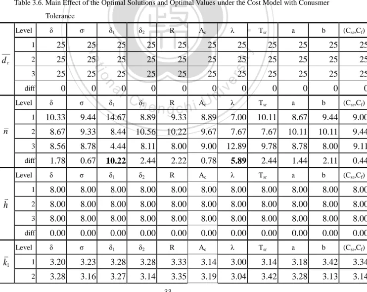
(7) LIST OF TABLES Table 2.1. Comparison of Three Types Design Charts under the Model without Tolerance .10 Table 2.2. The Optimal Solution of “Economic Statistic Economic. and S Charts” and “Shewhart-type. and S Charts” without Tolerance ..............................................................12. Table 2.3. The Optimal Solution and In-control Distribution of “Economic Statistic Charts” and “Shewhart-type economic. and S. and S Charts” without Tolerance .................14. Table 2.4. Input Parameters’ Levels Used in the Orthogonal Array ......................................15 Table 2.5. The Optimal Solutions for 27 Combinations of Input Parameters under the Cost Model without Tolerance ................................................................................................16 Table 2.6. Main Effect of the Optimal Solutions and Optimal Values under the Cost Model. 政治大. without Tolerance ...........................................................................................................17. 立. Table 2.7. The Significant Input Parameters of Each Design Parameter and EA under the Cost. ‧ 國. 學. Model without Tolerance ................................................................................................19 Table 3.1. Comparison of Three Types Design Charts under the Model with Consumer. ‧. Tolerance ........................................................................................................................25. y. and S Charts” and “Shewhart-type. and S Chart” with Consumer Tolerance ...................................................27. io. sit. Economic. Nat. Table 3.2. The Optimal Solution of “Economic Statistic. er. Table 3.3. The Optimal Solutions and In-control Distribution of “Economic Statistic. and S. n. a v Charts” and “Shewhart typel Economic and S chart” withi Consumer Tolerance ......29 n Ch e Combinations gchi U Table 3.4. Orthogonal Array L (3 ) for 27 n of Input Parameters ...................30 13. 27. Table 3.5. The Optimal Solutions for 27 Combinations of Input Parameters under the Cost Model with Consumer Tolerance ...................................................................................31 Table 3.6. Main Effect of the Optimal Solutions and Optimal Values under the Cost Model with Consumer Tolerance ...............................................................................................32 Table 3.7. The Significant Input Parameters of Each Design Parameter and EA under the Cost Model with Consumer Tolerance ...................................................................................34 Table 4.1. Comparison of Three Type Design Charts under the Model with Producer Tolerance ........................................................................................................................40. IV.

(8) Table 4.2. The Optimum Solution of “Economic Statistic Type Economic. and S Charts” and “Shewhart. and S Chart” with Producer Tolerance ............................................42. Table 4.3. The Optimum Solutions and In-Control Distribution of “Economic Statistic S Charts” and “Shewhart Type Economic. and. and S Chart” with Producer Tolerance ...44. Table 4.4. Orthogonal Array L27(313) for 27 Combinations of Input Parameters ...................45 Table 4.5. The Optimal Solutions for 27 Combinations of Input Parameters under the Cost Model with Producer Tolerance .....................................................................................46 Table 4.6. Main Effect of the Optimal Solutions and Optimal Values under the Cost Model with Producer Tolerance .................................................................................................47 Table 4.7. The Significant Input Parameters of Each Design Parameter and EA under the Cost. 政治大 Table 5.1.1. Comparison of Three 立 Types Design Charts under the Model with k = k , d > d , Model with Producer Tolerance .....................................................................................49 p. c. c. p. ‧ 國. 學. and Specified Ac > Determined Ap .................................................................................55 Table 5.1.2. The Optimum Solution of “Economic Statistic. and S Chart” with kp = kc, dc > dp, and Specified Ac >. ‧. “Shewhart-Type Economic. and S Charts” and. Determined Ap ................................................................................................................57. y. Nat. and S Chart” with kp = kc, dc > dp, and. al. er. io. and S Charts” and “Shewhart-Type Economic. sit. Table 5.1.3. The Optimum Solutions and In-Control Distribution of “Economic Statistic. iv n C Table 5.1.4. The Optimal Solutions for of Input Parameters under the Cost h27e Combinations ngchi U n. Specified Ac > Determined Ap ........................................................................................59. Model under the model “kp = kc, dc > dp, and Specified Ac > Determined Ap” ...............60. Table 5.1.5. Main Effect of the Optimal Solutions and Optimal Values under the model “kp = kc, dc > dp, and Specified Ac > Determined Ap” ..............................................................61 Table 5.1.6. The Significant Input Parameters of Each Design Parameters and EA under the model “kp = kc, dc > dp, and Specified Ac > Determined Ap” ............................................63 Table 5.2.1. Comparison of Three Type Design Charts under the Model with kc > kp, dc ≦ dp, and Specified Ac > Specified Ap .....................................................................................69 Table 5.2.2. The Optimum Solution of “Economic Statistic Type Economic. and S Charts” and “Shewhart. and S Chart” with kc > kp, dc ≦ dp, and Specified Ac > Specified Ap 71. V.

(9) Table 5.2.3. The Optimum Solutions and In-Control Distribution of “Economic Statistic and S Charts” and “Shewhart-Type Economic. and S Chart” with kc > kp, dc ≦ dp, and. Specified Ac > Specified Ap ............................................................................................73 Table 5.2.4. Orthogonal Array L27(313) for 27 Combinations of Input Parameters ................74 Table 5.2.5. The Optimal Solutions for 27 Combinations of Input Parameters under the Cost Model with kc > kp, dc ≦ dp, and Specified Ac > Specified Ap .......................................75 Table 5.2.6 Main Effect of The Optimal Solutions and Optimal Values under the Cost Model with kc > kp, dc ≦ dp, and Specified Ac > Specified Ap ...................................................76 Table 5.2.7. The Significant Input Parameters of Each Design Parameter and EA under the Cost Model with kc > kp, dc ≦ dp, and Specified Ac > Specified Ap ...............................78. 政治大 d ≦ d , and Specified A > Specified A .......................................................................87 立. Table 5.3.2.1. Comparison of Three Types Design Charts under the Cost Model with kc > kp, c. p. c. p. ‧ 國. “Shewhart-Type Economic. 學. Table 5.3.2.2. The Optimum Solution of “Economic Statistic. and S Charts” and. and S Chart” with kc > kp, dc > dp and specified Ac >. specified Ap .....................................................................................................................89. ‧. Table 5.3.2.3. The Optimum Solutions and In-Control Distribution of “Economic Statistic and S Chart” with kc > kp, dc > dp and. sit. y. Nat. and S Charts” and “Shewhart-Type Economic. al. er. io. Specified Ac > Specified Ap ............................................................................................91. v. n. Table 5.3.2.4. The Optimal Solutions for 27 Combinations of Input Parameters under the Cost. Ch. i Un. Model with kc > kp, dc > dp and Specified Ac > Specified Ap ..........................................92. engchi. Table 5.3.2.5. Main Effect of The Optimal Solutions and Optimal Values under the Cost Model with kc > kp, dc > dp and Specified Ac > Specified Ap ..........................................93 Table 5.3.2.6. The Significant Input Parameters of Each Design Parameter and EA under the Cost Model with kc > kp, dc > dp and Specified Ac > Specified Ap ..................................95 Table 5.3.3.1. Comparison of Three Types Design Charts under the Model with kp = kc, dc > dp, and Specified Ac > Specified Ap ...................................................................................101 Table 5.3.3.2. The Optimum Solution of “Economic Statistic Type Economic. and S Charts” and “Shewhart. and S Chart” with kp = kc, dc > dp, and Specified Ac > Specified Ap 103. VI.

(10) Table 5.3.3.3. The Optimum Solutions and In-Control Distribution of “Economic Statistic Aand S Charts” and “Shewhart-Type Economic. and S Chart” with kp = kc, dc > dp, and. Specified Ac > Specified Ap ..........................................................................................105 Table 5.3.3.4. The Optimal Solutions for 27 Combinations of Input Parameters under the Cost Model with kp = kc, dc > dp, and Specified Ac > Specified Ap .......................................106 Table 5.3.3.5. Main Effect of the Optimal Solutions and Optimal Values under the Cost Model with kp = kc, dc > dp, and Specified Ac > Specified A ........................................107 Table 5.3.3.6. The Significant Input Parameters of Each Design Parameter and EA under the Cost Model with kp = kc, dc > dp, and Specified Ac > Specified A ..................................109 Table 6.1. Compare all economic statistical design of. and S charts with a given n of the. 政治大. example .........................................................................................................................111. 立. ‧. ‧ 國. 學. n. er. io. sit. y. Nat. al. Ch. engchi. VII. i Un. v.

(11) LIST OF FIGURES Figure 2.1. Loss Function, In-control and Out-of-control Distributions ..................................5 Figure 2.2. Shewhart-Type Economic. and S Control Charts ..............................................8. Figure 2.3. Optimal Economic Statistical. and S Control Charts and with a Given n ..........9. Figure 3.1. Consumer Loss Function, In-control and Out-of-control Distributions ...............20 Figure 3.2. Shewhart-Type Economic. and S Control Charts with Consumer Tolerance ..23. Figure 3.3. Optimal Consumer Loss Function with In-control and Out-of-control Distributions ..........................................................................................................................................23 Figure 3.4. Optimal Economic Statistical. and S Control Charts with Consumer Tolerance. 治政大 Distributions ..............35 Figure 4.1. Producer Loss Function, In-Control and Out-Of-Control 立 and with a Given n ............................................................................................................24. Figure 4.2. Shewhart-Type Economic. and S Control Chart with Producer Tolerance .....38. ‧ 國. 學. Figure 4.3. Optimal Producer Loss Function with In-Control and Out-Of-Control Distributions ...................................................................................................................38. ‧. Figure 4.4. Optimal Economic Statistical. and S Control Charts with Producer Tolerance. Nat. sit. y. and with a Given n ..........................................................................................................39. n. al. er. io. Figure 5.1.1. Consumer Loss Function, Producer Loss Function, In-Control and. iv n U with Consumer and Producer eand n gS Control c h i Charts. Out-Of-Control Distributions .........................................................................................50. Ch Figure 5.1.2. Shewhart-Type Economic. Tolerances .........................................................................................................................53 Figure 5.1.3. Optimal Consumer and Producer Loss Function, In-Control and Out-Of-Control Distributions ...................................................................................................................53 Figure 5.1.3. Optimal Consumer and Producer Loss Function, In-Control and Out-Of-Control Distributions ...................................................................................................................53 Figure 5.1.4 Optimal Economic Statistical. and S Control Chart with Consumer and. Producer Tolerance and with a Given n ..........................................................................54 Figure 5.2.1. Consumer and Producer Loss Function, In-Control and Out-Of-Control Distributions ...................................................................................................................64. VIII.

(12) Figure 5.2.2. Shewhart-Type Economic. and S Control Charts with Consumer and Producer. Tolerances .......................................................................................................................67 Figure 5.2.3. Optimal Consumer and Producer Loss Function with In-Control and Out-Of-Control Distributions .........................................................................................67 Figure 5.2.4. Optimal Economic Statistical. and S Control Charts with Consumer and. Producer Tolerance and with a Given n ..........................................................................68 Figure 5.3.1.1. Consumer and Producer Loss Function, In-Control and Out-Of-Control Distributions ...................................................................................................................79 Figure 5.3.1. Consumer and Producer Loss Function, In-Control and Out-Of-Control Distributions ...................................................................................................................81 Charts with Consumer and 政 and治S Control 大 Producer Tolerance ...........................................................................................................84 立. Figure 5.3.2.2. Shewhart-Type Economic. ‧ 國. 學. Figure 5.3.2.3. Optimal Consumer and Producer Loss Function with In-Control and Out-Of-Control Distributions .........................................................................................84 and S Control Chart with Consumer and. ‧. Figure 5.3.2.4. Optimal Economic Statistical. Producer Tolerance and with a Given n ..........................................................................85. y. Nat. sit. Figure 5.3.2.5. Optimal Consumer and Producer Loss Function with In-Control and. er. io. Out-Of-Control Distributions .........................................................................................85. al. n. iv n C ................................................................................................................... 96 hengchi U. Figure 5.3.3.1. Consumer and Producer Loss Function, In-Control and Out-Of-Control Distributions. Figure 5.3.3.2. Shewhart-Type Economic. and S Control Chart with Consumer and. Producer Tolerances .......................................................................................................99 Figure 5.3.3.3. Optimal Consumer and Producer Loss Function with In-Control and Out-Of-Control Distributions .........................................................................................99 Figure 5.3.3.4. Optimal Economic Statistical. and S Control Charts with Consumer and. Producer Tolerance and with a Given n ........................................................................100 Figure 6.1. Main Effect Plot of Consumer Tolerance with Different Models ......................113 Figure 6.2. Main Effect Plot of Producer Tolerance with Different Models ........................113 Figure 6.3. Main Effect Plot of n Tolerance with Different Models ....................................113. IX.

(13) Figure 6.4. Main Effect Plot of h with Different Models .....................................................114 Figure 6.5. Main Effect Plot of k1 with Different Models ....................................................114 Figure 6.6. Main Effect Plot of k2 with Different Models ....................................................114 Figure 6.7. Main Effect Plot of k3 with Different Models ....................................................115 Figure 6.8. Main Effect Plot of False Alarm Rate with Different Models ...........................115 Figure 6.9. Main Effect Plot of True Alarm Rate with Different Models ............................115 Figure 6.10. Main Effect Plot of EA with Different Models ................................................116. 立. 政治大. ‧. ‧ 國. 學. n. er. io. sit. y. Nat. al. Ch. engchi. X. i Un. v.

(14) 1. INTRODUCTION AND LITERATURES REVIEW Control charts are widely used in statistical quality control. They monitor processes and determine whether a process is in-control or out-of-control. To use a control chart, the engineer must specify the sample size n, the sampling period h, and the coefficient of control limits k. In practice, these parameters are usually chosen by the engineer’s experience and by considering statistical criteria such as type I and type II errors. Duncan (1956) first recommended economic design of control charts. Duncan proposed a cost model to design the parameters of the control chart, which assumes that the assignable cause occurs according to the Poisson process. This cost model includes the cost of sampling and testing, the cost of finding the assignable cause, and the cost of process correction. Duncan’s work has been extensively studied and extended by many others.. 立. 政治大. ‧ 國. 學. After Duncan (1974) indicated that simultaneous employment of X and R charts to control process mean and variability “will give reasonably good control of the whole process,” joint economic design research has been conducted. Rahim et al.. sit. y. Nat. variability.. ‧. (1988) presented the use of joint economic designs of and S2 charts when the sample size is moderately large. Collani and Sheil (1989) proposed the economic design of an S chart when only a single assignable cause may influence process. n. al. er. io. When using economic design, the parameters of control charts should be determined by minimizing the expected cost from the process. This does not consider statistical properties such as Type I or Type II error rates. Woodall (1986, 1987) indicated that the Type I error rate of many economic control charts is higher than those of statistical design. Saniga (1979) proposed a method to design control charts that have bounds on Type I and Type II error probabilities and the average time to signal (ATS), but still allow for low-process variability and long-term quality. Although a design with these statistical constraints is more costly than economic. Ch. engchi. i Un. v. design, it is more effective and reduces false alarm rates. Saniga called this design “economic statistical design.” Elsayed and Chen (1994) found that the practical applications of economic design are limited because of difficulties in estimating costs. Quality loss is considered a cost when quality characteristic is not within the specification limits. Quality loss was defined by Taguchi (1984) as “the loss to society caused by the product after it is shipped out.” Taguchi proposed a quadratic loss function to estimate the quality loss of the manufactured product when it deviates from its target. Elsayed 1.

(15) and Chen (1994) proposed the economic design of charts based on the Taguchi loss function with continuous operations. Yang (1997) presented a joint economic design of and S charts with two assignable causes using the Taguchi quadratic loss function and presented a statistical constrained economic model that considers the Taguchi quadratic loss function for the optimal design of the S control chart for controlling process variability. In a complete inspection plan, every outgoing item is subjected to inspection, and items failing to meet the specifications are reworked. For items following a normal distribution, Tang (1988) presented an economic model to determine the most profitable specification for a complete inspection plan by considering quality loss. Fathi (1990) discussed producer tolerance and consumer tolerance, and proposed a graphical method to determine the producer tolerance for a given consumer tolerance by minimizing per-unit cost. Maghsoodloo and Li (2000) proposed an economic model for asymmetric tolerance design by minimizing the expected loss per unit.. 政治大. 立. ‧. ‧ 國. 學. Because the design of the process mean is an issue for engineering, Kapura (1988) proposed an economic model to determine process mean and tolerance simultaneously by minimizing per-unit costs under the symmetric Taguchi quadratic loss function. Lee, Kim, Kwon and Hong (2004) presented an economic model for a filling process to determine the process mean under specification is known by maximizing expected profit per unit. Furthermore, Feng and Kapura (2006) proposed an economic model to. y. Nat. al. er. io. sit. determine the mean and tolerance by minimizing expected cost per unit using an asymmetric quadratic Taguchi loss function and a piecewise linear loss function.. v. n. In a practical example, like pad is important for the Chemical Mechanical Polishing (CMP) of wafer. When the consumer gives an order for pad producer, they also give a consumer specification. Typically, producer specification is set with the same or less than consumer specification. If the nonconforming rate of wafer is high by using the pad of the CMP, the customer will ask to modify specification and the producer should re-determine their specification. Since that, the determination of consumer specification and producer specification is an important issue for producer.. Ch. engchi. i Un. The design of the control chart and specifications are both essential to quality control. Previous research has not discussed how to design them simultaneously. In this study, we propose economic cost models to design and S charts, consumer tolerance, and producer tolerance together. These models include the cases “only with consumer tolerance,” “only with producer tolerance,” and “with both producer and consumer tolerance.” We show the differences in the optimal costs, and differences in the optimal design parameters of specifications.. and S charts and producer and/or consumer 2.

(16) Section 2 of this study presents a discussion of an economic cost model without tolerance. This model is from Montgomery (1980) and Yang (1997). Sections 3 and 4 introduce a cost model with only consumer tolerance and a cost model with only producer tolerance. When we consider producer tolerance and consumer tolerance simultaneously, we assume that consumers and producers have different loss functions. Section 5 provides a discussion on different cost models for different relationships between consumer and producer loss functions. Section 6 shows a comparison of examples and sensitivity analysis for each model. Section 7 offers a conclusion.. 立. 政治大. ‧. ‧ 國. 學. n. er. io. sit. y. Nat. al. Ch. engchi. 3. i Un. v.

(17) 2. DESIGN OF ECONOMIC STATISTICAL TOLERANCE. AND S CHARTS WITHOUT. 2.1 Derivation of Cost Models We assume that the process begins in a statistical in-control state with mean μ and standard deviation σ. The time (Ts.c.) until the occurrence of assignable causes is exponential, with a mean of 1/λ. A single assignable cause shifts the mean from μ to μ + δ1σ (δ1 ≠ 0) and a shift of standard deviation from σ to δ2σ (δ2 > 1). Without loss of generality, we only consider the case of δ1 > 0 in this study. The quality characteristic is assumed to follow a normal distribution. This study assumes the following:.  . . X ~ N  , 2 , if process is in - control. X ~ N   1 ,  22 2 , 1  0,  2  1, if process is out - of - control.. . 立. 政治大. The samples of size n, unit time h, and the limits of the X and S charts are set. ‧ 國. 學.  n,  LCL X    k1 n. UCLX    k1. n. Ch. engchi. y. sit. io where 0  k3  k2 .. ‧. Nat. al. UCLS  k 2 , LCLS  k3. er. as. i Un. v. If at least one plotted point falls outside the control limits of the X and S charts, the process is assumed to be out-of-control and engineers must search for an assignable cause. If the process is out-of-control, corrective action is taken and the process continues. The probability (α) that at least one plotted point falls outside the control limits of the X and S charts when the process is in-control is calculated as follows:    X S  XS ,. where.     2(k1 ).  X  P X    k1 .    2  n X ~ N   ,    P X    k1    n   .   2  n X ~ N   ,    n   ,. 4.

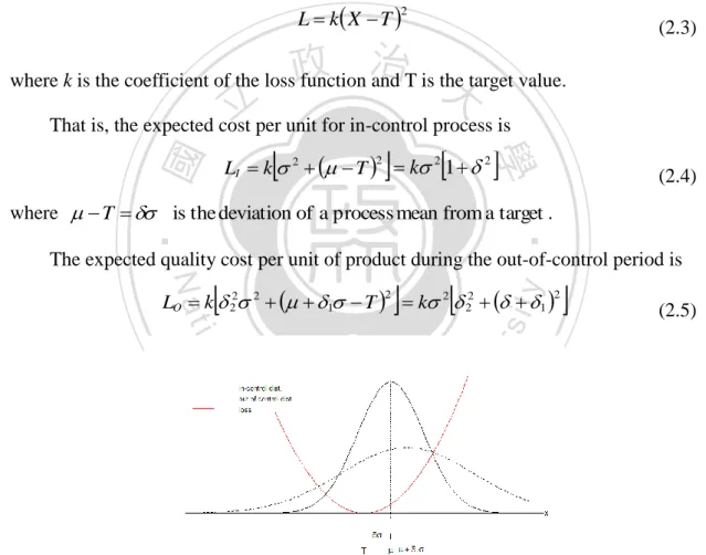
(18) .  . .  S  P s  k 2 X ~ N  ,  2   P s  k 3 X ~ N  ,  2   P(Y  (n  1)k 22 )  P(Y  (n  1)k 32 )  1  Fy ((n  1)k 22 )  Fy ((n  1)k 32 ). ,. where Y ~  n2-1 . The probability (β) that no sample points fall outside the control limits of the X and S charts when the process is out-of-control is calculated as follows:.    X S , where.    2 2   n  X    k1  n X ~ N     1 , 2    n      k  n 1    k  n 1     1    1 ,      2 2    .  X  P   k1 . 立. . 政治大 .  (n  1)k 32. ‧ 國. (n  1)k 22. (n  1)k 32.  22. ). (n  1)k 22    22  ,. sit. y. Nat. where Y ~  n2-1 ..  22. )  Fy (.  22. . Y . ‧.  Fy (. 學.  S  P k 3  s  k 2 X ~ N    1 ,  22 2   P. n. al. er. io. The expected number of false alarms that occur before a shift is α times the expected number of samples taken before a shift (1/λh).. Ch. i Un. v. The cycle time is defined as the time starts from in-control state and ends with the assignable cause is happened and repaired. A process is consisted of a series of independent and identical cycles. And the accumulated cost over the cycle is the expected cost. The process is called renewal reward process (Ross, 1993). In this article, the renewal approach is used to derive the expected cost per unit time.. engchi. Let ET be the expected cycle time, and let EC be the expected cost per cycle. And the optimal design parameters can be determined by minimizing the expected cost per unit time EA = EC / ET. The production cycle consists of three periods: (1) in-control period.  1 1 h   , and (3)   , (2) time to signal and out-of-control period h   1   2 12  time of searching and repairing assignable cause Ts.r . . Therefore, the expected cycle E (Ts.c. ) . 1. time is: 5.

(19) ET .  1   h     Ts.r .  1   1. (2.1). where the expected time of occurrence of the shift between j and j+1 sample is:. 1  1  h e  h h h 2   E Ts.c. | Ts.c.  h     2 12  1  e  h. . . (2.2). (Duncan, 1956) The expected quality loss per unit product can be easily estimated by the process variance and the deviation of process mean from the target, since we assume loss function (Figure 2.1) is. L  k X  T . 2. (2.3). 政治大. where k is the coefficient of the loss function and T is the target value.. 立. That is, the expected cost per unit for in-control process is. . . . ‧ 國. . 學. 2 LI  k  2    T   k 2 1   2. (2.4). ‧. where   T   is the deviation of a process mean from a target .. The expected quality cost per unit of product during the out-of-control period is. . . y. Nat. . io. n. al. 2. . (2.5). er. 2. sit. LO  k  22 2    1  T   k 2  22    1 . Ch. engchi. i Un. v. Figure 2.3. Loss Function, In-control and Out-of-control Distributions. The process costs, such as sampling and testing costs, false alarm costs, and assignable cause repair costs, are incurred in the cost model. We denote the costs for a cost model as follows: a = fixed cost of sampling and testing. b = cost per unit of sampling and testing. Cf = the cost of investigating a false alarm. 6.

(20) Csr = the cost of finding and repairing an assignable cause. The expected cost per cycle is the sum of (1) the total expected quality cost for the in-control period RL I. 1. . , (2) the total expected quality cost for the out-of-control.  h h h 2  period RLO   , (3) the total cycle cost of sampling and testing    1   2 12 .  1 1    , (4) the expected cost of false alarms during the cycle C f , (a  bn)  h  h 1    and (5) Csr. That is, EC  RL I.  h  1 h h 2  1     (a  bn)   C f  RLO      C sr (2.6)  h  h 1     1   2 12 . 政治大. 1. 立. ‧ 國. 學. where R = expected output per unit time. Hence, the expected cost per unit time is. ‧. y. sit. io. al. er. EC  ET.  h  1 h h 2  1     a  bn    C f  RLO      C sr  h  h 1     1   2 12  (2.7)  1 1 1 h    Ts.r .  h     1   2 12  1. Nat. EA . RL I. v. n. The economic statistical design parameters can be determined by minimizing the cost function (2.7). A subroutine “DEoptim” in R program (Ardia et al., 2011), which is an optimization method based on a differential evolution algorithm, is used to solve the object. The upper bound of α is set to αU, and the upper bound of β is set to βU. The lower and upper bounds of n, h, k1, k2, and k3 are set to nU, hU, k1U, and k2U. The upper bound of k2 is determined by the same cumulative probability of k1. Therefore, the. Ch. engchi. i Un. optimization model is expressed as. min EA n, h, k1 , k 2 , k3  s.t. nL  n  nU , 0  h  hU , 0  k1  k1U , 0  k3  k 2  k 2U ,   U ,   U . 7.

(21) 2.2 An Example and Numerical Analysis 2.2.1 Example In this section, we give an example to show the application of the economic statistical X and S control charts without tolerance. We compare the optimal solutions and the expected costs of three types of X and S control charts: (1) Shewhart-type economic X and S control charts with design h, (2) economic statistical X and S control charts with a given n, and (3) economic statistical X and S control charts with all design parameters. A subroutine “DEoptim” in R program is used to determine the optimal solutions in the optimization models. This study uses data from Montgomery (2009). The data were the standardized filling heights of soft drinks. Data were obtained from 15 subgroups of size 10 (= n), with a process mean of 0, a variance of 1, and a target value of 0. Other input parameters of the cost function were δ1 = 1.5, δ2 = 2, k = 4, R = 30, λ = 0.01, Tsr = 3, a. 立. 政治大. = 0.5, b = 0.1, Csr = 35, and Cf = 50.. ‧ 國. 學. (1) Shewhart-type economic X and S control charts with design h. ‧. To construct the Shewhart-type economic X and S charts when n = 10 and α = 0.00539 (  X =  S = 0.0027), we calculated that k1 = 3, k2 = 1.735, k3 = 0.371, and β =. n. al. er. io. min EA(h) s.t. 0  h  8 .. sit. y. Nat. 0.06502. The expected cost per unit time of the optimal Shewhart-type economic X and S charts is. i Un. v. The EA* is 110.903, and h* is 8. The optimal Shewhart-type economic X and S charts are constructed as follows.. Ch. engchi. UCLX  3 UCLS  1.735 and LCL X  3 LCLS  0.371 Plotting the data in Shewhart-type economic X and S control charts shows whether they are in-control. Figure 2.2 shows that no points fall outside the limits of Shewhart-type economic X and S control charts, thus indicating that these charts can be used to monitor the future process.. 8.

(22) Figure 4.2. Shewhart-type Economic. and S Control Charts. (2) Economic statistical X and S control charts with a given n. 治政 function to construct the economic statistical X and大 S control charts. The expected 立 economic statistical X and S charts is cost per unit time of the optimal The design parameters are determined with a given n by minimizing the cost. sit. Nat. y. ‧. ‧ 國. 學. min EA h, k1 , k 2 , k3  s.t. 0  h  8, 0  k1  4, 0  k 3  k 2  4.2,   0.01,   0.2.. The optimal design parameters are h* = 8, k1* = 3.581, k2* = 2.194, k3* = 0.017,. io. n. al. er. α* = 0.00013, and β* = 0.2. The EA* is 109.572. The optimal economic statistical X and S charts are constructed as follows.. Ch. engchi. i Un. v. UCLS  2.194 UCLX  3.581 and LCLS  0.0017 LCLX  3.581 Figure 2.3 shows the optimal economic statistical X and S control charts. No points fall outside the limits of the optimal charts... 9.

(23) Figure 2.3. Optimal Economic Statistical. and S Control Charts and with a Given n. (3) Economic statistical X and S control charts with all determined design parameters. 政治大. Assuming that all design parameters can be determined by minimizing the cost. 立. y. sit er. ‧ 國. io. al. ‧. Nat. min EA n, h, k1 , k 2 , k3  s.t. 2  n  25, 0  h  8, 0  k1  4 , 0  k3  k 2  4.2 , α  0.01, β  0.2.. 學. function, the expected cost per unit time of the optimal economic statistical X and S charts is. n. iv n C 0.00184, β* = 0.2, and the EA* is 109.556. h e n gThec optimal i U economic statistical h S charts are constructed as follows.. The parameters are n* = 7, h* = 8, k1* = 3.300, k2* = 1.949, k3* = 0.0003, α* = X and. UCLS  1.949 UCLX  3.300 and LCLS  0.0003 LCLX  3.300 Finally, we compare “Shewhart-type economic charts” and “economic statistical charts with a given n” leads to finding (i) and (ii). Comparing economic statistical chart with all design parameters and with a given n leads to finding (iii) (See Table 2.1): (i) If producer can design the chart, k1* and k2* should increase, k3* should decrease and EA* will reduce.. 10.

(24) (ii) Using Economic statistical and s chart without design n, EA* could save about 1.2%. And the false alarm rate of economic statistical chart without design n will decrease, but the true alarm rate will decrease. (iii) If producer can decide all design parameter of control chart, n* should decrease from 10 to 7, k1* and k2* should be decrease and EA* will reduce.. Table 2.1. Comparison of Three Types Design Charts under the Model without Tolerance. n (1) Shewhart-type economic X and S control charts. h* 10. n (2) Economic statistical X and S control charts with a given n. 立. 3. k1*. k3. 1.735. 0.371 0.00539. k* 治政 8 3.581 2.194 大 10 h* 7. k1* 8. 3.300. k3*. 2. k2* 1.949. y. sit er. n. engchi. 11. i Un. α*. 0.000 0.00184. ‧. io. Ch. α*. 0.017 0.00034. k3*. Nat. al. α. k2. 學. ‧ 國. 8. h*. n*. (3) Economic statistical X and S control charts with all design parameters. k1. v. β 0.06502. β* 0.20000. β* 0.20000. EA* 110.903. EA* 109.572. EA* 109.556.

(25) 2.2.2 The Effects of Optimal Design Parameters under Different Combinations of δ and σ for a Given In-control Distribution This section sets the process mean and variance in different combinations to show the manner in which the process mean and variance affect the design parameters and the expected cost. Furthermore, it compares these optimal economic statistical control charts with Shewhart-type economic control charts, which fix the false alarm rate of each chart under 0.0027. Input parameters are from Montgomery (1985), and other input parameters of the cost function are T = 0, δ1 = 1.5, δ2 = 2, k = 4, R = 30, λ = 0.01, Ts.r. = 3, a = 0.5, b = 0.1, Csr = 35, and Cf = 50. The results of these objects are shown in Table 2.2. Comparing the optimal solutions of economic statistical and S charts under different combinations of process mean and variance leads to following findings:. 政治大. (i) Under δ equals to 0, when σ decreases from 2 to 1, n* and h* will not change, the width of. 立. and S charts will be smaller, and EA* will reduce about 75%.. ‧ 國. width of. 學. (ii) Under δ equals to 1, when σ decreases from 2 to 1, n* and h* will not change, the and S charts will be smaller, and EA* will reduce about 75%.. and S charts will be a little larger, and EA* will reduce about 47%.. Nat. y. width of. ‧. (iii) Under σ equals to 1, when σ increases from 0 to 1, n* and h* will not change, the. n. al. er. and S charts will be a little larger, and EA* will reduce about 47%.. io. width of. sit. (iv) Under σ equals to 2, when σ increases from 0 to 1, n* and h* will not change, the. i Un. v. Comparing economic statistical control charts with Shewhart-type economic control charts base on same combination of process mean and variance leads to following findings: (v) EA* of economic statistical economic and S charts’.. Ch. engchi. and S charts are a little higher than Shewhart-type. (vi) The false alarm rate of Economic Statistic alarm rate is smaller, too.. and S chart is smaller, but its true. According to the findings (i)-(iv), if a producer can only improve mean or variance, it should decrease variance first because this can reduce costs more than improving the mean can. If a producer improves the variance, the producer should reduce the width of the and S charts. If a producer improves the deviation of the mean and target, the producer should increase the width of the and S charts. According to findings (v)-(vi), The expected costs of the two charts are similar. 12.

(26) Producers are advised to use the Shewhart-type economic the convenience of using the chart. Table 2.2. The Optimal Solution of “Economic Statistic. Economic Statistical. 7. 8. 7. UCL*X. LCL*X. UCL*S. LCL*S. (k1*). (k1*). (k2*). (k3*). 6.572. -6.572. 3.91. 0.004. (3.286). (3.286). (1.955). (0.002). 3.3. -3.3. 1.949. 0. (3.3). (3.3). (1.949). (0). 7.59. -5.59. 3.902. 0.002. (3.295). (1.951). (0.001). (3.296). (1.951). (0). 8. 7. 8. (3.295). (4) δ=1 and σ=1. 7. 立4.296. 8. 政治大 -2.296 1.951 0. 7. 8. 7. LCLX. UCLS. LCLS. (k1). (k1). (k2). (k3). 6. -6. 3.806. 0.532. (3). (3). (1.903). (0.266). 3. -3. 1.903. 0.266. (3). (3). (1.903). (0.266). -5. 3.806. 8. n (3) δ=1 and σ=2. 7. 8. (4) δ=1 and σ=1. 7. 8. 4 (3). 0.532 iv n e(3)n g c(1.903) h i U (0.266) -2. 1.903. 0.266. (3). (1.903). (0.266). 13. 0.00184. 0.20000. 437.239. 0.00184. 0.20000. 109.556. 0.00184. 0.20000. 830.977. 0.00184. 0.20000. 207.990. α. β. EA*. 0.00539. 0.16024. 438.851. 0.00539. 0.16024. 109.977. 0.00539. 0.16024. 836.533. 0.00539. 0.16024. 209.397. and S Control Charts. UCLX. al 7 Ch (3). EA*. ‧. h*. io. (2) δ=0 and σ=1. n*. Nat. (1) δ=0 and σ=2. Shewhart-Type Economic. β*. 學. ‧ 國. (3.296). α*. y. h*. sit. (3) δ=1 and σ=2. n*. and S Control Charts. er. (2) δ=0 and σ=1. and S Charts” and “Shewhart-Type. and S Charts” without Tolerance. Economic. (1) δ=0 and σ=2. or S charts depending on.

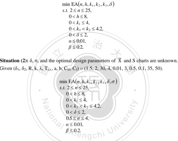
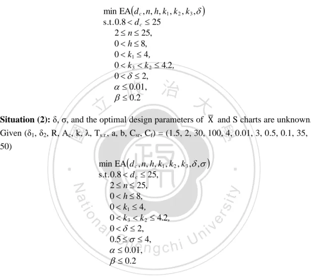
(27) 2.2.3 Determining Optimal in Control Distribution with Minimum Expected Cost Per Unit Time. This section determines the optimal solutions for 2 situations. Situation (1): σ is known, δ is unknown, and the optimal design parameters of and S charts are unknown. Given (σ, δ1, δ2, R, k, λ, Ts.r., a, b, Csr, Cf) = (2, 1.5, 2, 30, 4, 0.01, 3, 0.5, 0.1, 35, 50).. min EA n, h, k1 , k 2 , k 3 ,   s.t. 2  n  25, 0  h  8, 0  k1  4, 0  k 3  k 2  4.2 , 0  δ  2, α  0.01, β  0.2.. 立. 政治大. Situation (2): δ, σ, and the optimal design parameters of. and S charts are unknown.. n. Ch. engchi. y. sit. io. al. er. Nat. min EA n, h, k1 , k 2 , k 3 ,  ,   s.t. 2  n  25, 0  h  8, 0  k1  4 , 0  k 3  k 2  4.2 , 0  δ  2, 0.5  σ  4 , α  0.01, β  0.2.. ‧. ‧ 國. 學. Given (δ1, δ2, R, k, λ, Ts.r., a, b, Csr, Cf) = (1.5, 2, 30, 4, 0.01, 3, 0.5, 0.1, 35, 50).. i Un. v. To determine the optimal solutions in above models, we use a subroutine “DEoptim” in R program. Table 2.3 shows the optimal solutions of 2 situations and leads to the following findings: (i) In situation (1), the δ* is approximately 0. This means that if a producer can design a process mean, it should choose a mean as close to the target as possible. (ii) In situation (2), δ* is approximately 0 and σ* is 0.5. This means that if a producer can design the mean and variance, μ* should be as close to the target as possible, and σ* should be small.. 14.

(28) (iii) Compare situation (1) to (1) in Table 2.2, when μ is unknown, n* increases, h* decreases, the width of the chart decreases, and the width of the S chart increases, but EA* is smaller for μ = T. (iv) Compare situation (2) to (1) in Table 2.2, when μ and σ are unknown, n* increases, h* decreases, the width of the chart increases, and EA* is smaller.. chart decreases, the width of the S. Table 2.3. The Optimal Solution and In-control Distribution of “Economic Statistic and S Charts” without Tolerance. Economic Statistical. δ*. σ*. n*. h*. UCL*X. LCL*X. -4.942E. 0.500. unknown. 立. 0.311. -16. 9. (3.251). (3.251). (1.795). (0.003). 1.6265. -1.6265. 0.8975. 0.002. (3.253). (3.253). (1.795). 1.250. io. 1.512E 0.500. unknown. -16. 9. EA*. 0.00230. 0.10701. 475.800. 0.00228. 0.10729. 31.801. α. β. EA*. 0.00539. 0.08853. 476.087. 0.00539. 0.08853. 31.872. (0.004). and S Control Charts. UCLX. LCLX. UCLS. LCLS. (k1). (k1). (k2). (k3). 6. -6. 3.56. 0.682. (3). (3). (1.780). 0.333. (0.341). 1.5 -1.5 0.89 a1.338 v 0.1705 i l C (3) (3) (1.780) (0.341) hengchi Un. n. (2) δ and σ are. -15. 9. h*. β*. er. --. unknown (σ=2). n*. Nat. (1) σ is known, δ is 1.394E. σ*. α*. 0.006. ‧. δ*. (k3*). 1. Shewhart-Type economic. situation. (k2*). 學. (2) δ and σ are. -16. ‧ 國. unknown (σ=2). 9. LCL*S. (k *) (k *) 治政 6.502 -6.502 3.59 大 1. (1) σ is known, δ is 4.778E. UCL*S. y. situation. and S Control Charts. sit. and “Shewhart-type economic. and S Charts”. 15.

(29) 2.3 Sensitivity Analysis The economic cost model without tolerance requires the user to specify 11 costs and process parameters. This section uses an orthogonal array to study the effects and sensitivities of the input parameters (δ, σ, δ1, δ2, R, λ, Tsr, a, b, Csr, and Cf) on the design parameters and expected cost per unit time. Table 2.4 shows three levels of each parameter. Because the cost of false alarms and cost of searching and repairing an assignable cause are correlated, these two parameters’ levels are set in combination. Other parameters are assumed to be independent. Table 2.4. Input Parameters’ Levels Used in the Orthogonal Array. Level Input parameter. 2 2.5 2.5 2 500 0.1 1 100. 0.1 (35,50). 1 (50,25). n. y. sit. er. io. 1 1 30 0.01 3 0.5. 1 2 1.5 1.5 100 0.05 2 50. ‧. Nat. b (Csr, Cf). al. 3. 0 政治 1 大. ‧ 國. 立. 2. 學. δ σ δ1 δ2 R λ Tsr a. 1. Ch. engchi. 16. i Un. v. 5 (100,40).

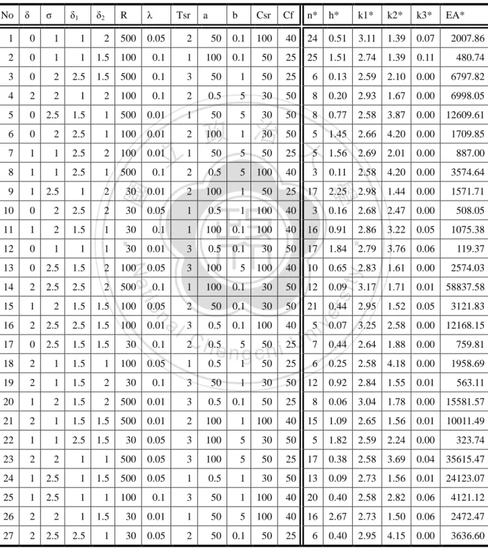
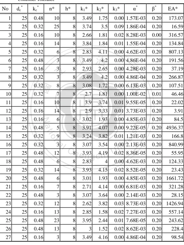
(30) 13. An orthogonal array table L27(3 ) is used for sensitivity analysis. Table 2.5 shows the optimal solutions for these 27 combinations of input parameters.. Table 2.5. The Optimal Solutions for 27 Combinations of Input Parmaters under the Cost Model without Tolerance δ. σ. δ1. δ2. R. λ. Tsr. a. b. Csr. Cf. n*. h*. k1*. k2*. k3*. EA*. 1. 0. 1. 1. 2. 500. 0.05. 2. 50. 0.1. 100. 40. 24. 0.51. 3.11. 1.39. 0.07. 2007.86. 2. 0. 1. 1. 1.5. 100. 0.1. 1. 100. 0.1. 50. 25. 25. 1.51. 2.74. 1.39. 0.11. 480.74. 3. 0. 2. 2.5. 1.5. 500. 0.1. 3. 50. 1. 50. 25. 6. 0.13. 2.59. 2.10. 0.00. 6797.82. 4. 2. 2. 1. 2. 100. 0.1. 2. 0.5. 5. 30. 50. 8. 0.20. 2.93. 1.67. 0.00. 6998.05. 5. 0. 2.5. 1.5. 1. 500. 0.01. 1. 50. 5. 30. 50. 8. 0.77. 2.58. 3.87. 0.00. 12609.61. 6. 0. 2. 2.5. 1. 100. 0.01. 2. 1.45. 2.66. 4.20. 0.00. 1709.85. 7. 1. 1. 2.5. 2. 100. 0.01. 1.56. 2.69. 2.01. 0.00. 887.00. 8. 1. 1. 2.5. 1. 500. 9. 1. 2.5. 1. 2. 10. 0. 2. 2.5. 2. 11. 1. 2. 1.5. 1. 12. 0. 1. 1. 1. ‧ 國. No. 13. 0. 2.5. 1.5. 2. 100. 14. 2. 2.5. 2.5. 2. 15. 1. 2. 1.5. 16. 2. 2.5. 17. 0. 18. 40. 3. 0.11. 2.58. 4.20. 0.00. 3574.64. 2.25. 1.44. 0.00. 1571.71. 0.16. 2.68. 2.47. 0.00. 508.05. 2. 100. 1. 50. 25. 17. 2.98. 30. 0.05. 1. 0.5. 1. 100. 40. 3. 30. 0.1. 1. 100. 0.1. 100. 40. 16. 0.91. 2.86. 3.22. 0.05. 1075.38. 30. 0.01. 3. 0.5. 0.1. 30. 50. 17. 1.84. 2.79. 3.76. 0.06. 119.37. 0.05. 3. 100. 5. 100. 40. 10. 0.65. 2.83. 1.61. 0.00. 2574.03. 500. 0.1. 1. 100. 0.1. 30. 50. 12. 0.09. 3.17. 1.71. 0.01. 58837.58. 1.5. 100. 2. 50. 0.1. 30. 50. 21. 0.44. 2.95. 1.52. 0.05. 3121.83. 2.5. 1.5. 100. 0.01. 3. 0.5. 0.1. 100. 40. 3.25. 2.58. 0.00. 12168.15. 2.5. 1.5. 1.5. 30. 0.1. 2. v0.07 i n. 2. 1. 1.5. 1. 100. 19. 2. 1. 1.5. 2. 20. 1. 2. 1.5. 21. 2. 1. 22. 1. 23. n. al. er. 0.05. ‧. 0.01. Nat. 30. y. 100. 學. 5. io. 0.5. sit. 1 立 0.1 2. 100 1 治 30 50 5 政 50 5 50 25 大 5. 5. 0.44. 2.64. 1.88. 0.00. 759.81. 0.05. C h0.5 5 50 25U 7 engchi. 1. 0.5. 1. 50. 25. 6. 0.25. 2.58. 4.18. 0.00. 1958.69. 30. 0.1. 3. 50. 1. 30. 50. 12. 0.92. 2.84. 1.55. 0.01. 563.11. 2. 500. 0.01. 3. 0.5. 0.1. 50. 25. 8. 0.06. 3.04. 1.78. 0.00. 15581.57. 1.5. 1.5. 500. 0.01. 2. 100. 1. 100. 40. 15. 1.09. 2.65. 1.56. 0.01. 10011.49. 1. 2.5. 1.5. 30. 0.05. 3. 100. 5. 30. 50. 5. 1.82. 2.59. 2.24. 0.00. 323.74. 2. 2. 1. 1. 500. 0.05. 3. 100. 5. 50. 25. 17. 0.38. 2.58. 3.69. 0.04. 35615.47. 24. 1. 2.5. 1. 1.5. 500. 0.05. 1. 0.5. 1. 30. 50. 13. 0.09. 2.73. 1.56. 0.01. 24123.07. 25. 1. 2.5. 1. 1. 100. 0.1. 3. 50. 1. 100. 40. 20. 0.40. 2.58. 2.82. 0.06. 4121.12. 26. 2. 2. 1. 1.5. 30. 0.01. 1. 50. 5. 100. 40. 16. 2.67. 2.73. 1.50. 0.06. 2472.47. 27. 2. 2.5. 2.5. 1. 30. 0.05. 2. 50. 0.1. 50. 25. 6. 0.40. 2.95. 4.15. 0.00. 3636.60. 17.

(31) Table 2.6 shows the main effects of the optimal solutions and optimal values for three input parameter levels and it shows the following findings: (i) δ1 is significant to average sample size n*. When δ1 increases, average n* decreases. (ii) R, λ and a are significant to average sampling interval h*. When R, λ, or a increase, average h* decreases. (iii) δ2 is significant to average k1* and k2*. When δ2 increases, optimum average k1* increases and average k2* decreases. (iv) All input parameters are significant to average EA*. When δ, σ, R, or λ increase, average EA* increases. When b increases, average EA* decreases. When δ1, δ2, Tsr, or a increase, average EA *decreases first and then increases.. 立. 政治大. 3. 10.78. diff. 1.22. 11.00. 10.67. 11.11. 11.44. 12.56. 11.67. 11.67. 10.89. 5.56. 11.00. 11.78. 12.11. 1.56. 11.89. 1.67. 0.78. 1.44. σ 0.83. 1.07. 2. 0.85. 0.71. 3. 0.67. 0.57. diff. 0.17. 0.49. δ. σ. δ1. δ2. R. λ. Tsr 11.11. δ1. 0.21. 0.91. δ2. R. 0.78 λ. b. (Csr,Cf). 7.78. 14.89. 11.22. 11.78. 13.11. 10.78. 10.78. 11.56. 13.56. 8.78. 12.44. 5.78. 6.11. 1.67. 0.67. Tsr. 0.72 1.27 1.31 a1.09 l0.61C 0.92 0.73 n0.52i v hengchi U 0.64 0.71 0.36 0.52 0.48. a. a. b. (Csr,Cf). 0.70. 0.36. 0.65. 0.85. 0.77. 0.87. 0.75. 0.78. 0.89. 1.13. 0.96. 0.73. 0.19. 0.77. 0.31. 0.12. Tsr. a. b. (Csr,Cf). 1. 2.74. 2.73. 2.80. 2.68. 2.78. 2.82. 2.79. 2.80. 2.99. 2.80. 2. 2.78. 2.78. 2.77. 2.76. 2.80. 2.78. 2.83. 2.78. 2.70. 2.75. 3. 2.85. 2.85. 2.80. 2.92. 2.78. 2.77. 2.75. 2.78. 2.68. 2.81. diff. 0.12. 0.12. 0.02. 0.24. 0.02. 0.05. 0.08. 0.02. 0.30. 0.05. Level. k2. 10.89. 1. Level. k1. 17.44. n.  h. δ. 12.44. io. Level. λ. y. 12.00. R. sit. 2. δ2. er. 11.67. δ1. Nat. 1. σ. ‧. n. δ. ‧ 國. Level. 學. Table 2.6. Main Effect of the Optimal Solutions and Optimal Values under the Cost Model without Tolerance. δ. σ. δ1. δ2. R. λ. Tsr. a. b. (Csr,Cf). 1. 2.52. 2.48. 2.14. 3.79. 2.47. 2.52. 2.46. 2.68. 2.39. 2.45. 2. 2.31. 2.46. 2.35. 1.81. 2.44. 2.54. 2.45. 2.32. 2.43. 2.51. 3. 2.51. 2.40. 2.85. 1.74. 2.43. 2.28. 2.43. 2.34. 2.52. 2.37. diff. 0.21. 0.07. 0.71. 2.05. 0.04. 0.25. 0.03. 0.35. 0.13. 0.14. 18.

(32) Level. R. λ. Tsr. a. b. (Csr,Cf). 0.03. 0.05. 0.02. 0.02. 0.01. 0.02. 0.01. 0.04. 0.01. 2. 0.02. 0.02. 0.01. 0.03. 0.02. 0.02. 0.02. 0.03. 0.01. 0.02. 3. 0.01. 0.01. 0.00. 0.01. 0.02. 0.03. 0.03. 0.02. 0.01. 0.03. diff. 0.01. 0.02. 0.04. 0.02. 0.01. 0.01. 0.01. 0.02. 0.03. 0.01. δ. σ. δ1. δ2. R. λ. Tsr. a. b. (Csr,Cf). 1. 0.0088. 0.0091. 0.0091. 0.0078. 0.0080. 0.0076. 0.0079. 0.0079. 0.0046. 0.0077. 2. 0.0081. 0.0078. 0.0081. 0.0083. 0.0081. 0.0081. 0.0079. 0.0082. 0.0097. 0.0087. 3. 0.0074. 0.0074. 0.0071. 0.0081. 0.0082. 0.0085. 0.0085. 0.0083. 0.0100. 0.0079. diff. 0.0014. 0.0017. 0.0020. 0.0005. 0.0001. 0.0009. 0.0006. 0.0004. 0.0054. 0.0010. δ. σ. δ1. δ2. R. 0.0434. 0.0754. 2. 0.0491. 0.0693. 0.0590. 3. 0.0629. 0.0589. 0.0372. 0.0632 0.0561 治 0.0669 政大 0.0630 0.0510 0.0500. diff. 0.0139. 0.0259. 0.0382. 0.0178. σ. δ1. 0.0134. δ2. R. 0.0546. 0.0169 λ. a. b. (Csr,Cf). 0.0492. 0.1224. 0.0325. 0.0591. 0.0449. 0.0295. 0.0622. 0.0622. 0.0774. 0.0198. 0.0769. 0.0503. 0.0325. 0.1026. 0.0445. 0.0119. 學. δ. 0.0645. Tsr. 0.0596. 立. 0.0454. λ. 1. Level. Tsr. a. b. (Csr,Cf). 3063.02. 2214.07. 8612.21. 7157.86. 1225.58. 6347.91. 8651.60. 7310.16 10781.01 12045.13. 2. 6042.23. 8208.94. 5361.72. 6695.46. 3779.94. 8207.70. 3710.20. 4024.16. 5707.21. 7476.60. 3 14695.73 13377.97. 9827.05. 9947.66 18795.46. 9245.36 11439.18 12466.67. 7312.76. 4279.24. diff 11632.72 11163.89. 4465.33. 3252.20 17569.87. 2897.45. 5073.80. 7765.89. y. 7728.97. n. al. er. io. sit. Nat. 1. ‧. EA. δ2. 0.03. Level. . δ1. 1. Level. . σ. ‧ 國. k3. δ. Ch. engchi. 19. i Un. v. 8442.51.

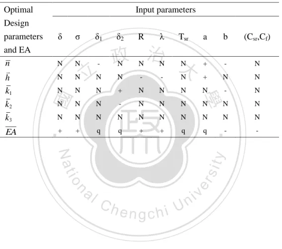
(33) In Table 2.6, if the input parameter is significant to optimal design parameter and their relationship is linear and positive, we use notation “+”, if the input parameter is significant and their relationship is linear and negative, we use notation “-“, and if the input parameter is significant and their relationship is quadratic, we use notation “q“; otherwise, we use notation “N”.. Table 2.7. The Significant Input Parameters of Each Design Parameter and EA. Optimal δ1. N. N. -. N. N. 立N. N. N. N. δ2. R. λ. Tsr. 治N N 政 N N 大. a. b. (Csr,Cf). +. -. N. N. -. -. N. +. N. N. N. +. N. N. N. N. -. N. N. N. -. N. N. N. N. N. N. N. N. N. N. N. N. N. N. N. N. +. +. q. q. +. +. q. q. -. ‧ 國. Nat. io. sit. y. -. n. al. er. EA. σ. ‧. k2 k3. δ. 學. Design parameters and EA n  h k1. Input parameters. Ch. engchi. 20. i Un. v.

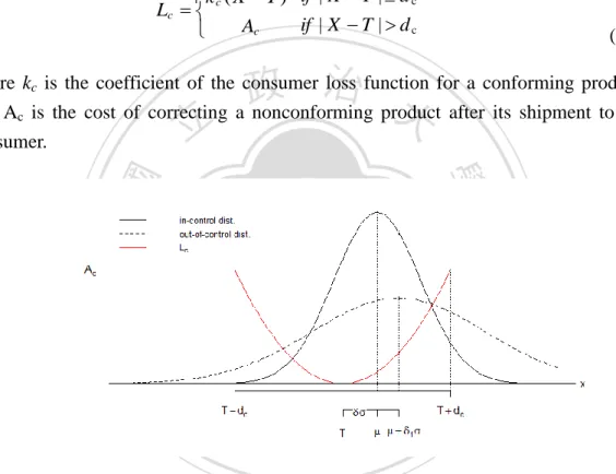
(34) 3.. DESIGN. OF. STATISTICAL. CONSUMER. TOLERANCE. AND. ECONOMIC. AND S CHARTS. 3.1 Derivation of Cost Models The assumptions of process distributions and economic statistical X and S charts continue to hold in this section. A consumer tolerance dc is assumed to exist such that if |X-T|> dc, the product is nonconforming for consumers. T+ dc and T- dc are the consumer specification limits (Fathi, 1990). Let Lc denote the consumer quadratic loss function (Figure 3.1). k c ( X  T ) 2 if | X  T |  d c Lc   if | X  T |  d c Ac . (3.1). 治政大 after its shipment to the and A is the cost of correcting a nonconforming product 立 consumer.. where kc is the coefficient of the consumer loss function for a conforming product, c. ‧. ‧ 國. 學. n. er. io. sit. y. Nat. al. Ch. i Un. engchi. v. Figure 3.1. Consumer Loss Function, In-control and Out-of-control Distributions. The expected cost per unit while the process is in-control is shown in (3.2), and the expected per unit cost while the process is out-of-control is shown in (3.3): LI  Ac 1  P(T  d c  X  T  d c )  k c . T dc. T dc. k c ( x  T ) 2 f X ( x)dx. d    c    dc  2  Ac    ( z )dz   dc  ( z )dz   k c  dc z   2  ( z )dz         . 21. (3.2).

(35) LO  Ac 1  P(T  d c  X  T  d c )  . T dc. T dc. k c ( x   ) 2 f X ( x)dx.  1   1  dc      ( z ) dz   Ac    2  1 d c   ( z ) dz      1   2     . (3.3). 1 dc    1     dc    1   2   .  k c 2  12.  2 z     1 2  ( z )dz. Hence, the expected cost per unit time is. R EA .  h  1 h h 2  1     (a  bn)  RLO      Csr   C f  1   2 12  h 1    h     (3.4)  1 1 1 h   h     Tsr   1   2 12 . LI. The design parameters can be determined by minimizing the cost function (3.4). A subroutine “DEoptim” in R program is used to solve the object. The upper bound of. 政治大 α is set to α , and the upper bound of β is set to β . The upper bounds of d , n, h, k , k , 立 and k are set to d , n , h , k , and k . The lower bound of d and n are d , n . Let U. 3. U. cU. U. U. 1U. c. 2. c. 1. cL. 2. L. n. al. y. er. io. sit. Nat. min EA d c , n, h, k1 , k 2 , k 3  s.t. d cL  d c  d cU , n L  n  nU , 0  h  hU , 0  k1  k1U , 0  k3  k 2  k 2 U ,   U , iv n C h   U . U. ‧. ‧ 國. 學. the rate of nonconforming products for consumers be smaller than 0.1, the bounds of dc can be determined. Therefore, the optimization model is expressed as follows:. engchi. 22.

(36) 3.2 An Example and Numerical Analysis 3.2.1 Example In this section, we give an example to show the application of the economic statistical X and S control chart only with consumer tolerance. We compare the optimal solutions and the expected costs per unit time of three types of X and S control charts: (1) Shewhart-type economic X and S control charts with design h and dc, (2) economic statistical X and S control charts with a given n, and (3) economic statistical X and S control charts with all design parameters. A subroutine “DEoptim” in R program is used to determine the optimal solutions in the optimization models. The data which we use in this section is the same as 2.2.1, and the input parameters are set by δ1=1.5, δ2=2, Ac=100, R=30, λ=0.01, Tsr=3, a=0.5, b=0.1, Csr=35, and Cf=50.. 立. (1) Shewhart-type economic X. 政治大 and S control charts with design h and d. c. ‧ 國. 學. To construct the Shewhart-type economic X and S charts when n = 10 and α = 0.00539 (  X =  S = 0.0027), we calculated that k1 = 3, k2 = 1.735, k3 = 0.371, and β =. sit. io. al. er. Nat. min EA(d c , h) s.t. 0.8  d c  25, 0  h  8.. y. ‧. 0.06502. The expected cost per unit time of the optimum Shewhart-type economic X and S charts is. n. iv n C nonconforming product is 0, andhthe Shewhart-type economic i U e noptimal h c g charts are constructed as follows.. The EA* is 4.817, h* is 8, and dc* is 25. Under the dc*, the calculated rate of X and S. UCLS  1.735 UCLX  3 and LCLS  0.371 LCLX  3 Plotting the data in Shewhart-type control charts shows whether they are in-control. Figure 3.2 shows that no points fall outside the limits of Shewhart-type X and S control charts, thus indicating that these charts can be used to monitor the future process. Figure 3.3 shows that all products fall into the consumer specification.. 23.

(37) Figure 3.2. Shewhart type Economic. 立. and S Control Charts with Consumer Tolerance. 政治大. ‧. ‧ 國. 學 sit. y. Nat. er. io. Figure 3.3. Optimal Consumer Loss Function with In-control and Out-of-control Distributions. al. n. iv n C The design parameters are determined U n by minimizing the cost h e n g cwith h ia given function to construct the economic statistical X and S control charts. The expected (2) Economic statistical X and S control charts with a given n. cost per unit time of the optimal economic statistical X and S charts is. min EA d c , h, k1 , k 2 , k3  s.t. 0.8  d c  25, 0  h  8, 0  k1  4, 0  k3  k2  4.2,   0.01,   0.2. The optimal design parameters are dc* = 25, h* = 8, k1* = 4, k2* = 2.001, k3* = 0.005, α* = 0.00001, and β* = 0.2. The EA* is 4.712. The optimal economic statistical X and S charts are constructed as follows.. 24.

(38) UCLX  4 UCLS  2.001 and LCLX  4 LCLS  0.005 . Figure 3.4 shows the optimal economic statistical X and S control charts. No points fall outside the limits of the optimal charts. Because the optimal consumer tolerance is the same as the previous, all in-control and out-of-control products are in the consumer specification limits.. 立. 政治大. and S Control Charts with Consumer Tolerance and. ‧. ‧ 國. 學. Figure 3.4. Optimal Economic Statistical. with a Given n. Nat. sit. y. (3) Economic statistical X and S control charts with all design parameters. er. io. Assuming that all design parameters can be determined by minimizing the cost function, the expected cost per unit time of the optimal economic statistical X and S charts is. n. al. Ch. engchi. i Un. v. min EA d c , n, h, k 1 , k 2 , k 3  s.t. 0.8  d c  25, 2  n  25, 0  h  8, 0  k1  4, 0  k 3  k 2  4.2 , α  0.01, β  0.2.. The parameters are dc* = 25, n* = 7, h* = 8, k1* = 3.300, k2* = 1.949, k3* = 0.001, α* = 0.00186, and β* = 0.2. The EA* is 4.697. Under the dc*, the rate of nonconforming product is 0, and the optimal economic statistical X and S charts are. UCLX  3.300 UCLS  1.949 and LCLX  3.300 LCLS  0.001 25.

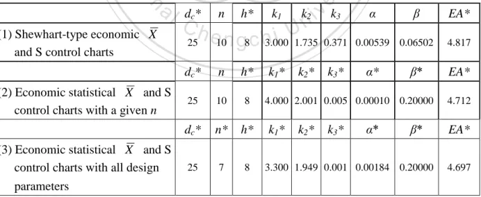
(39) Finally, we compare the optimal solutions and the EA* of these three types design charts (See Table 3.1). Comparing with “Shewhart-type” and “economic statistical chart with a given n” leads to following findings: (i) If producer can design the chart, k1* and k2* should increase, k3* should decrease and EA* will reduce. (ii) Using economic statistical and S charts with given n, EA* could save about 2.1%. And the false alarm rate of economic statistical chart with given n will decrease, but the true alarm rate will decrease. (iii) The optimal consumer tolerance all equals to 25.. 政治大. Comparing economic statistical chart with design n and with given n leads to following findings:. 立. ‧ 國. 學. (iv) If producer can decide all design parameter of control chart, n* should decrease, k1* and k2* should be decrease and EA* will reduce.. ‧. Because the EA* cannot be saved a lot when we use economic statistical control chart with consumer tolerance, we advise that it is more convenience for using Shewhart-type economic control chart and let consumer tolerance equal to 25.. io. sit. y. Nat. n. al. (1) Shewhart-type economic X and S control charts (2) Economic statistical X and S control charts with a given n (3) Economic statistical X and S control charts with all design parameters. er. Table 3.1. Comparison of Three Types Design Charts under the Model with Consumer Tolerance. dc*. Ch 25. n. h*. k1. i e10n g8c h3.000. dc*. n. h*. 25. 10. 8. dc*. n*. h*. 25. 7. 8. 26. k1*. i Un. v k3. k2*. k3*. k2. α. β. 1.735 0.371 0.00539 0.06502. α*. β*. 4.000 2.001 0.005 0.00010 0.20000. k1*. k2*. k3*. α*. β*. 3.300 1.949 0.001 0.00184 0.20000. EA* 4.817. EA* 4.712. EA* 4.697.

(40) 3.2.2 The Effects of Optimal Design Parameters under Different Combination δ and σ for a Given In-control Distribution This section sets the process mean and variance in different combinations to show the manner in which the process mean and variance affect the design parameters and the expected cost. Furthermore, it compares these optimal economic statistical control charts with Shewhart-type economic control charts, which fix the false alarm rate of each chart under 0.0027. Other input parameters of the cost function are Ac = 100, T = 0, δ1 = 1.5, δ2 = 2, k = 4, R = 30, λ = 0.01, Tsr = 3, a = 0.5, b = 0.1, Csr = 35, and Cf = 50. The results of these objects are shown in Table 3.2. Comparing the optimal solutions of economic statistical and S charts under different combinations of process mean and variance leads to the following findings:. 政治大 (i) Under δ equals to 0, when σ decreases from 2 to 1, d *, n* and h* will not change, 立 the width of and S charts will be smaller, and EA* will reduce about 74%. c. ‧ 國. 學. (ii) Under δ equals to 1, when σ decreases from 2 to 1, dc*, n* and h* will not change, the width of. and S charts will be smaller, and EA* will reduce about 74%.. ‧. sit. y. Nat. (iii) Under σ equals to 1, when σ increases from 0 to 1, dc*, n*, h* and the width of and S charts will not change, EA* will reduce about 46%.. n. al. er. io. (iv) Under σ equals to 2, when σ increases from 0 to 1, dc*, n*, h* and the width of and S charts will not change, and EA* will reduce about 47%.. Ch. i Un. v. Comparing with economic statistical control charts and Shewhart-type economic control charts base on same combination of process mean and variance leads to the following findings (v) EA* of economic statistical economic and s charts’. (vi) The α* of Economic Statistic. engchi. and S charts are a little higher than Shewhart-type. and s chart is smaller, but its β* is smaller, too.. According to the findings (i)-(iv), decreasing variance can reduce costs more than improving the mean can. If a producer improves the variance, the producer should reduce the width of the and S charts. In all situations, optimal consumer tolerance equals to 25 and all products are in the consumer specification limits. According to findings (v)-(vi), the expected costs of the two charts are similar. Producers are advised to use the Shewhart-type economic the convenience of using the chart. 27. or S charts depending on.