行政院國家科學委員會專題研究計畫 成果報告
動態類神經網路在非線性系統鑑別與控制器設計之應用
研究成果報告(精簡版)
計 畫 類 別 : 個別型 計 畫 編 號 : NSC 98-2221-E-009-126- 執 行 期 間 : 98 年 08 月 01 日至 99 年 07 月 31 日 執 行 單 位 : 國立交通大學電機與控制工程學系(所) 計 畫 主 持 人 : 王啟旭 計畫參與人員: 碩士班研究生-兼任助理人員:黃繼輝 博士班研究生-兼任助理人員:洪&;#22531;能 報 告 附 件 : 出席國際會議研究心得報告及發表論文 處 理 方 式 : 本計畫可公開查詢中 華 民 國 99 年 12 月 23 日
行政院國家科學委員會補助專題研究計畫
; 成 果 報 告
□
期中進度報告
動態類神經網路在非線性系統鑑別與控制器設計之應用
Application of Dynamic Neural Network Model for Nonlinear System Identification and Control
計畫類別:
;
個別型計畫 □ 整合型計畫
計畫編號:NSC
98-2221-E-009-126-執行期間: 98 年 8 月 1 日至 99 年 7 月 31 日
計畫主持人:王啟旭
共同主持人:
計畫參與人員:
成果報告類型(依經費核定清單規定繳交):
;
精簡報告 □完整報告
本成果報告包括以下應繳交之附件:
□赴國外出差或研習心得報告一份
□赴大陸地區出差或研習心得報告一份
□出席國際學術會議心得報告及發表之論文各一份
□國際合作研究計畫國外研究報告書一份
處理方式:除產學合作研究計畫、提升產業技術及人才培育研究計畫、
列管計畫及下列情形者外,得立即公開查詢
□涉及專利或其他智慧財產權,□一年□二年後可公開查詢
執行單位:國立交通大學 電機工程學系
中 華 民 國 九 十 九 年 十 月 十 四 日
Application of Dynamic Neural Network Model for Nonlinear System
Identification and Control
Abstract
The Hopfield neural network (HNN) has been widely discussed for controlling a nonlinear dynamical system. The weighting factors in HNN will be tuned via the Lyapunov stability criterion to guarantee the convergence performance. The proposed architecture in this paper is high-order Hopfield-based neural network (HOHNN), in which additional inputs from functional link net for each neuron are considered. Compared to HNN, the HOHNN performs faster convergence rate. The simulation results for both HNN and HOHNN show the effectiveness of HOHNN controller for affine nonlinear system. It is obvious from the simulation results that the performance for HOHNN controller is better than HNN controller.
1. Introduction
The Hopfield neural network (HNN) consists of a set of neuron and a corresponding set of unit delays forming a multiple-loop feedback system where the number of feedback loops is equal to the number of neurons. The HNN proposed in 1982 [1] has been adopted for pattern recognition [2], and image processing [3] in recent years. Neural networks, like HNNs, are suitable for controlling nonlinear dynamical systems due to their learning and memorizing capabilities.
Functional link net methodology was first proposed in 1989 [4, 5] which have been combined with the neural network to create the high-order neural networks (HONNs). The input pattern of a functional link net an expansion of original input variables in HNN. There have been many considerable interests in exploring the applications of functional link model to deal with nonlinearity and uncertainties. The advantages of high-order functional link net have been shown in [6], in which the efficiency of supervised learning is not only greatly improved, but a flat net without hidden layer is also capable enough of doing the same job. However the functional link neural networks in [7] does not include the Hopfield neural network (HNN), and the weighting factors tuned via back-propagation algorithm can not guarantee the convergence of the nonlinear dynamical systems, especially in the real-time applications.
In this paper, a new high-order Hopfield-based neural network (HOHNN) is proposed. It is basically a HNN with the compact functional link net and its exact analytical expression is also proposed. The application of HOHNN controller is explored in this paper to show the advantages of extra inputs for each neuron in HOHNN. A Lyapunov-based tuning algorithm is then proposed to find the optimal weighting matrix of HOHNN controller to achieve favorable approximation error. Furthermore, the convergence analysis with tuning weighting factors in the HOHNN controller is
considered. The simulation results for both HNN and HOHNN controllers are finally conducted to show that the HOHNN controller has better effective performance for nonlinear dynamical system than HNN controller.
2. Hopfield-based Network Models
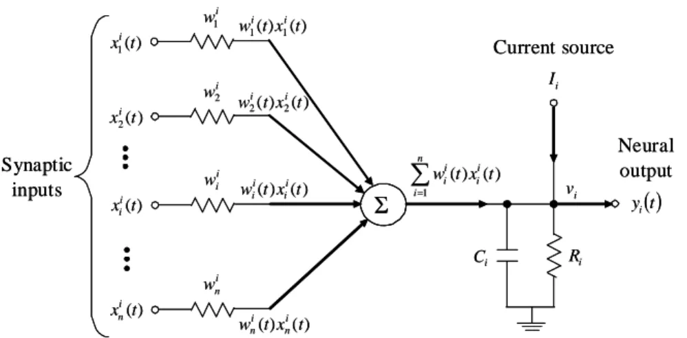
Based on their feedback link connection architecture, there are three different types of artificial neural networks. We focus attention on the recurren Hopfield-based neural network in this paper. Considering the noiseless dynamic model of a single neuron in HNN illustrated in Fig. 1, the input vector represent
voltages, the weighting vector represent
conductance, and n represents the number of neurons. The input vector are fed back from the output vector
] ) ( ) ( ) ( [ ) (t x1 t x2 t x t x in i i i K = ] ) ( ) ( ) ( [ ) (t w1 t w2 t w t w ni i i i K = ) (t xi ] ) ( ) ( ) ( [ ) (t y1 t y2 t y t y = K n
, and a current source Ii represents the externally applied bias.
Σ ) ( 1t xi w1(t)x1(t) i i i w1 ) ( 2t xi w2(t)x2(t) i i i w2 ) (t xi i i i w ) ( ) (t x t w i i i i ) (t xin ) ( ) (tx t wi i i n w n n ∑ = n i i i i i t x t w 1 ) ( ) ( ( )t yi i v Neural output i R i C Synaptic inputs Current source i I ΣΣ ) ( 1t xi w1(t)x1(t) i i i w1 ) ( 2t xi w2(t)x2(t) i i i w2 ) (t xi i i i w ) ( ) (t x t w i i i i ) (t xin ) ( ) (tx t wi i i n w n n ∑ = n i i i i i t x t w 1 ) ( ) ( ( )t yi i v Neural output i R i C Synaptic inputs Current source i I
Fig. 1. The ith neuron in a Hopfield neural network.
The nonlinear function ϕ(⋅) is a sigmoid function which limits the amplitude range of the sum of inputs is defined by hyperbolic tangent function:
⎟ ⎠ ⎞ ⎜ ⎝ ⎛ = 2 tanh ) ( i i i v a v ϕ (1)
where refers to the gain of iai >0 th
neuron. By the Kirchhoff’s current law, the following dynamic node equation can be obtained:
i n i i i i i i i w t x t I R t v dt t dv C + =
∑
+ =1 ) ( ) ( ) ( ) ( , i=1,L,n. (2)i n i i i i i i i w t v t I R t v dt t dv C + =
∑
+ =1 )) ( ( ) ( ) ( ) ( ϕ , i=1,L,n. (3) The stability analysis of the above HNN has been proved in [8], in which an energy function was defined and it derivative function can be shown to be negative to yield an asymptotical stable system.3. The Compact Functional Link Net with HNN
The functional link net is a single layer structure in which the hidden layer is removed. However, such functional transforms greatly increases the dimensions of input vector. Hence, it was suggested in [4] that high-order terms beyond the second-order term are not required in the enhanced patterns of input vector and the terms with two or more equal indices are also omitted. Therefore, a compact functional link net can be defined with rigorous formulae as shown in the following Fig. 2 and equations. The input pattern vector Z in Fig. 2 can be defined precisely as follows:
( )⎥ ⎦ ⎤ ⎢ ⎣ ⎡ = + + 2 1 1 2 1 z zN zN zN N z L L Z (4) and
{
}
{
}
. ) 1 ( ,..., 2 , 1 | ,..., 2 , 1 | 2 ,..., 2 , 1 | 1 ,..., 2 , 1 | 1 1 1 2 ) 2 )( 1 ( ) 1 ( 2 ) 1 ( 2 2 2 ) 1 2 ( 1 1 1 1 1 4 2 2 1 1 ⎪⎭ ⎪ ⎬ ⎫ ⎪⎩ ⎪ ⎨ ⎧ − − = = ⎪⎭ ⎪ ⎬ ⎫ ⎪⎩ ⎪ ⎨ ⎧ − = = − = = − = = − − + − + ⎥⎦ ⎤ ⎢⎣ ⎡ − − − − + + ⎥⎦ ⎤ ⎢⎣ ⎡ − − + + − + + − − N N z z z k N z z z N z z z N z z z N N N N N N N k k k k k kN N N N N k l L l L l l l l l l l l l l (5) ] [z1 z2 L zN = Z Input patternFunctional link net
1 z z2 L zN z1z2 L zN−1zN L L 1 w w2
L
NL
w wN+1 wN(N+1)/2 Enhanced pattern v Output node Weighting factor ] [z1 z2 L zN = Z Input patternFunctional link net
1 z z2 L zN z1z2 L zN−1zN L L 1 w w2
L
NL
w wN+1 wN(N+1)/2 Enhanced pattern v Output node Weighting factorFig. 2. A compact structure of functional link net.
Equation (4) says that the dimension of Z vector is N (N + 1) / 2, in which N is the number of original input variables. All the extra second order terms in (5) for
( ) ⎭ ⎬ ⎫ ⎩ ⎨ ⎧ + + + 2 1 2 1 N N N N z z
z L are described. Further we let the input vector of HNN in
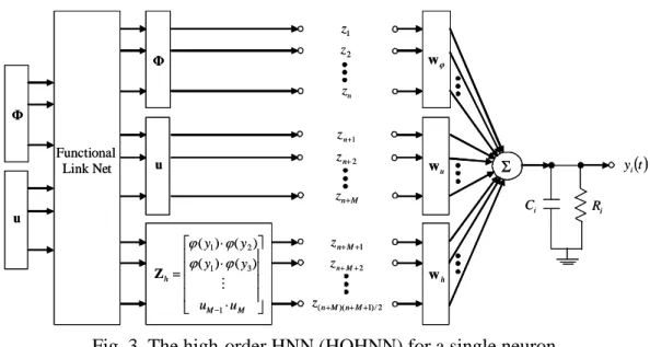
Fig. 1 to form a compact functional link net defined in Fig. 2. This combination in HOHNN structure for a single neuron is shown in the following Fig. 3.
Σ yi( )t i R i C Functional Link Net 2 z 2 / ) 1 )( (n+M n+M+ z n z 1 + n z M n z+ 2 + + M n z 1 z 2 + n z 1 + +M n z ⎥ ⎥ ⎥ ⎥ ⎦ ⎤ ⎢ ⎢ ⎢ ⎢ ⎣ ⎡ ⋅ ⋅ ⋅ = − M M h u u y y y y 1 3 1 2 1 ) ( ) ( ) ( ) ( M ϕ ϕ ϕ ϕ Z ϕ w u w h w u Φ u Φ ΣΣ yi( )t i R i C Functional Link Net 2 z 2 / ) 1 )( (n+M n+M+ z n z 1 + n z M n z+ 2 + + M n z 1 z 2 + n z 1 + +M n z ⎥ ⎥ ⎥ ⎥ ⎦ ⎤ ⎢ ⎢ ⎢ ⎢ ⎣ ⎡ ⋅ ⋅ ⋅ = − M M h u u y y y y 1 3 1 2 1 ) ( ) ( ) ( ) ( M ϕ ϕ ϕ ϕ Z ϕ w u w h w u Φ u Φ
Fig. 3. The high-order HNN (HOHNN) for a single neuron.
The input pattern of HOHNN produced from functional link net is the enhanced pattern in which is the n-dimension vector of the network feedback, u is the M-dimension vector of the input; and is the high-order term vectors to the system in Fig. 3. For this compact functional link net, the dimension of input vector has been expanded to N = (n + M) (n + M + 1) / 2. Thus, the N-dimension input vector Z and
the n × N matrix of weighting factor matrix can be defined as
Φ h Z
[
]
T h Z u Φ Z= (6) and ] [w wu wh W = ϕ (7)where , , and represent the weighting factors of feedback input, error input and high-order term, respectively.
ϕ
w wu wh
The structure of HOHNN in Fig. 4 can be expressed as h T h T u T Z Bw u Bw Φ Bw Ax x& = + ϕ + + . (8)
where is a Hurwitz matrix with
; and with n n n R a a a diag − − − ∈ × = { 1 2 L } A ) /( 1 i i i RC a = n n n R b b b diag ∈ × = { 1 2 L } B bi =1/Ci. The output of
each neuron in HOHNN can be expressed as
h T i h i T i u i T i i i i i ax b b b x& =− + wϕ, Φ+ w , u+ w , Z , i=1,2,K,n (9) where , , and are the i
T i , ϕ w T i u, w T i h, w th
rows of , , and , respectively. Solve the differential equation (8), we obtain
ϕ w wu wh n i b e x e b x i h T i h i u T i u i T i i t a i t a i h T i h i u T i u i T i i i i i , , 2 , 1 ), ( ) ( 0 , , 0 , , 0 , , 0 , , , , , , K = + + − + + + = − − ζ w ζ w ζ w ζ w ζ w ζ w ϕ ϕ ϕ ϕ (10)
where is the initial state of ;
0 i x xi n i∈R , ϕ ζ , M i u, ∈R ζ , and ( )( 1)/2 , − + + ∈ n M n M i h R ζ are
the solutions of ζ&ϕ,i =−aiζϕ,i+Φ , ζ&u,i =−aiζu,i+u , and ζ&h,i =−aiζh,i+Zh ,
respectively; 0 ,i ϕ ζ , 0 ,i u ζ , and 0 ,i h
ζ are initial states of ζϕ,i, ζu ,i, and ζh,i, respectively.
Note that 0 i t a x e− i and ( ) 0 , , 0 , , 0 , , hi T i h i u T i u i T i i t a b e−i w ζ +w ζ +w ζ ϕ ϕ in (10) will exponentially
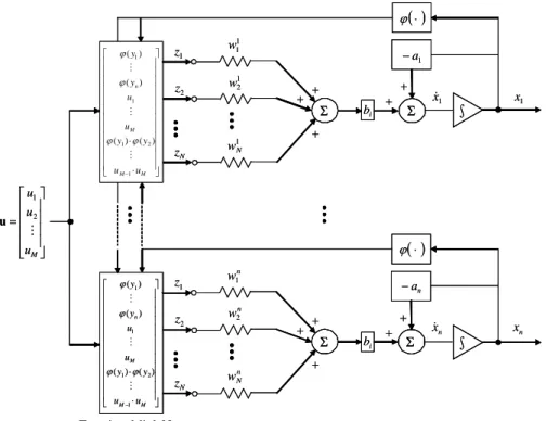
⎥ ⎥ ⎥ ⎥ ⎦ ⎤ ⎢ ⎢ ⎢ ⎢ ⎣ ⎡ = M u u u M 2 1 u Σ 1 1 w 1 2 w 1 N w + 1 x ( ) ⋅ ϕ + + ⎥ ⎥ ⎥ ⎥ ⎥ ⎥ ⎥ ⎥ ⎥ ⎥ ⎥ ⎥ ⎦ ⎤ ⎢ ⎢ ⎢ ⎢ ⎢ ⎢ ⎢ ⎢ ⎢ ⎢ ⎢ ⎢ ⎣ ⎡ ⋅ ⋅ − M M M n u u y y u u y y 1 2 1 1 1 ) ( ) ( ) ( ) ( M M M ϕ ϕ ϕ ϕ Functional-link Net Σ n w1 n w2 n N w + n x ( ) ⋅ ϕ + + ⎥ ⎥ ⎥ ⎥ ⎥ ⎥ ⎥ ⎥ ⎥ ⎥ ⎥ ⎥ ⎦ ⎤ ⎢ ⎢ ⎢ ⎢ ⎢ ⎢ ⎢ ⎢ ⎢ ⎢ ⎢ ⎢ ⎣ ⎡ ⋅ ⋅ − M M M n u u y y u u y y 1 2 1 1 1 ) ( ) ( ) ( ) ( M M M ϕ ϕ ϕ ϕ 1 z 2 z N z 1 z 2 z N z i b i b 1 x& n x& Σ Σ ∫ ∫ 1 a − n a − + + + + ⎥ ⎥ ⎥ ⎥ ⎦ ⎤ ⎢ ⎢ ⎢ ⎢ ⎣ ⎡ = M u u u M 2 1 u ΣΣ 1 1 w 1 2 w 1 N w + 1 x ( ) ⋅ ϕ + + ⎥ ⎥ ⎥ ⎥ ⎥ ⎥ ⎥ ⎥ ⎥ ⎥ ⎥ ⎥ ⎦ ⎤ ⎢ ⎢ ⎢ ⎢ ⎢ ⎢ ⎢ ⎢ ⎢ ⎢ ⎢ ⎢ ⎣ ⎡ ⋅ ⋅ − M M M n u u y y u u y y 1 2 1 1 1 ) ( ) ( ) ( ) ( M M M ϕ ϕ ϕ ϕ Functional-link Net ΣΣ n w1 n w2 n N w + n x ( ) ⋅ ϕ + + ⎥ ⎥ ⎥ ⎥ ⎥ ⎥ ⎥ ⎥ ⎥ ⎥ ⎥ ⎥ ⎦ ⎤ ⎢ ⎢ ⎢ ⎢ ⎢ ⎢ ⎢ ⎢ ⎢ ⎢ ⎢ ⎢ ⎣ ⎡ ⋅ ⋅ − M M M n u u y y u u y y 1 2 1 1 1 ) ( ) ( ) ( ) ( M M M ϕ ϕ ϕ ϕ 1 z 2 z N z 1 z 2 z N z i b i b 1 x& n x& ΣΣ ΣΣ ∫ ∫ ∫ ∫ 1 a − n a − + + + +
Fig. 4. The structure of HOHNN.
Consider the nth-order nonlinear dynamical system of the following form:
x y d gu f xn = + + = ) ( ) ( x (11)
where is the system state vector, the nonlinear function describes the system dynamics,
T n x x x ] [ 1 2 L = x R R
f : n → u∈R is a continuous control input of
the system, and is a bounded external disturbance. In order for (11) to be controllable and without losing generality, it is required that
R d∈ ∞ < < g 0 . The control objective is to force the system output y to follow a given bounded reference signal
. The reference signal vector and the error vector e are defined as r y yr n T n (12) R e e e ∈ = − ] , , , [ &K ( 1) e
with . If the function f (x) and g are known and the system is free
of external disturbance, the ideal controller can be designed as
y y x y e= r − = r − T T c n r ideal f y g u = 1[− (x)+ ( ) +k e] (13)
where . Applying (13) to (11), we have the following error dynamical system T n n c =[k ,k −1,K,k1] k (14) 0 ) 1 ( 1 ) ( + − + + = e k e k en n L n
n n n k s k s s
H( )≅ + 1 −1+L+ lie strictly in the left half of the complex plane, then
0 ) ( lim = ∞ → e t
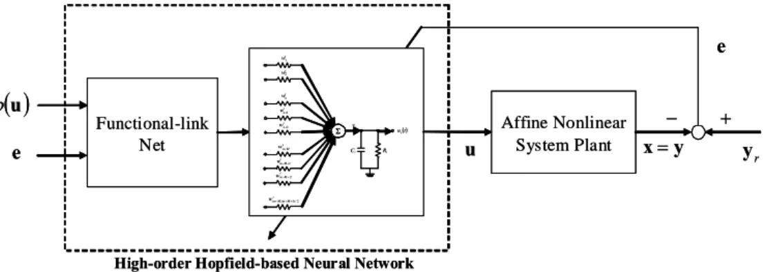
t can be implied for any initial conditions. However, since the system dynamics may be unknown or perturbed, the ideal controller uideal in (13) cannot be implemented. In order to control the unknown nonlinear system, an HOHNN with single layer, fully connection, recurrent nets and functional link model is proposed. The overall closed-loop diagram of direct adaptive HOHNN controller for affine nonlinear system is shown in the following Fig. 5.
Affine Nonlinear System Plant u Functional-link Net x=y − + ( )u ϕ e
High-order Hopfield-based Neural Network
r y e Σ i w1 i w2 i n w+1 i M n M n w(+) (++1)/2 ( )t ui i v i R i C i n w i n w+2 i M n w+ i M n w++1 i M n w++2 Affine Nonlinear System Plant u Functional-link Net x=y − + ( )u ϕ e
High-order Hopfield-based Neural Network
r y e Σ i w1 i w2 i n w+1 i M n M n w(+) (++1)/2 ( )t ui i v i R i C i n w i n w+2 i M n w+ i M n w++1 i M n w++2 ΣΣ i w1 i w2 i n w+1 i M n M n w(+) (++1)/2 ( )t ui i v i R i C i n w i n w+2 i M n w+ i M n w++1 i M n w++2
Fig. 5. The closed-loop configuration of HOHNN controller for affine nonlinear system.
Substituting u=uideal into (11) and using (13) yields
d u u gB ideal B Ae e&= + ( − )− =Ae+gBu~−Bd (15) where n n n n n k k k k − − ⎥ × ⎥ ⎥ ⎥ ⎦ ⎤ ⎢ ⎢ ⎢ ⎢ ⎣ ⎡ − − − − = 1 2 1 1 0 0 0 0 0 0 1 0 L L O O O M L A , 1 1 0 0 × ⎥ ⎥ ⎥ ⎥ ⎦ ⎤ ⎢ ⎢ ⎢ ⎢ ⎣ ⎡ = n M
B , and u~=uideal −u. Note that
the ideal controller is a scalar, and thus the HOHNN controller contains only a single neuron. The input signals shown in the HOHNN controller shown in Fig. 3 are
ideal u
[
]
T n u u u ) ( ) ( ) ( 1 ϕ 2 ϕ ϕ L = Φ ,[
]
T M e e e1 2 L = u[
M]
T e e e ( −1) = & L , and[
]
T M M n h = ϕ(u1)⋅ϕ(u2) L ϕ(u1)⋅ϕ(u ) L L e −1⋅e Z . (16)where Zh vector in (16) comes from (5) in the compact functional link net shown in Fig. 2. The output signal can be expressed as
) ˆ ˆ ˆ ( 1 ) ˆ ˆ ˆ ( 1 0 0 0 1 0 1 h h u u t RC t RC h h u u C e u e C u= wϕζϕ +w ζ +w ζ + − − − wϕζϕ +w ζ +w ζ . (17)
where is the initial value of u;
0
u wˆϕ, wˆϕ, and wˆϕ are the estimations of wϕ, wϕ,
and wϕ. Substituting (17) into (15) yields
d e C e C e C g RCt h h h u t RC u u t RCζ w ζ ζ w ζ ζ B ζ w B Ae e − ⎥ ⎥ ⎦ ⎤ Δ + ⎟⎟ ⎠ ⎞ ⎜⎜ ⎝ ⎛ − + ⎢ ⎢ ⎣ ⎡ ⎟⎟ ⎠ ⎞ ⎜⎜ ⎝ ⎛ − + ⎟⎟ ⎠ ⎞ ⎜⎜ ⎝ ⎛ − + = − − − 0 1 0 1 0 1 ~ 1 ~ 1 ~ 1 ϕ ϕ ϕ & (18)
where is the control error. In order to derive the one of main theorems in the following section, the following assumption is required.
Δ
Assumption: Let ε =Δ− g1d . Assume that there exists a finite constant μ so that μ τ ε ≤
∫
t d 0 2 , ≤ t <∞ 0 . (19)The constraint set for wˆϕ , wˆu , and wˆh are Ωϕ ={wˆϕ :wˆϕ ≤Mwϕ} ,
} ˆ : ˆ { u M u u u w w w Ω = ≤ , and {ˆ : ˆ } h M h h h w w w
Ω = ≤ . If the adaptive laws are
designed as
(
)
⎪ ⎪ ⎩ ⎪ ⎪ ⎨ ⎧ ⎟ ⎟ ⎠ ⎞ ⎜ ⎜ ⎝ ⎛ < ⎟ ⎟ ⎠ ⎞ ⎜ ⎜ ⎝ ⎛ − = ⎥ ⎥ ⎦ ⎤ ⎢ ⎢ ⎣ ⎡ ⎟ ⎟ ⎠ ⎞ ⎜ ⎜ ⎝ ⎛ − ⎟ ⎟ ⎠ ⎞ ⎜ ⎜ ⎝ ⎛ ≥ ⎟ ⎟ ⎠ ⎞ ⎜ ⎜ ⎝ ⎛ − = < ⎟ ⎟ ⎠ ⎞ ⎜ ⎜ ⎝ ⎛ − = − = − − − − 0 ˆ and ˆ if 0 ˆ and ˆ or ˆ if ~ ˆ 0 1 0 1 0 1 0 1 ϕ ϕ ϕ ϕ ϕ ϕ ϕ ϕ ϕ ϕ ϕ ϕ ϕ ϕ ϕ ϕ ϕ ϕ ϕ ϕ β β ζ ζ w PB e w ζ ζ PB e Pr ζ ζ w PB e w w ζ ζ PB e w w w w w t RC T t RC T t RC T t RC T e M e C e M M e C & & (20)(
)
⎪ ⎪ ⎩ ⎪ ⎪ ⎨ ⎧ ⎟ ⎟ ⎠ ⎞ ⎜ ⎜ ⎝ ⎛ < ⎟⎟ ⎠ ⎞ ⎜⎜ ⎝ ⎛ − = ⎥ ⎥ ⎦ ⎤ ⎢ ⎢ ⎣ ⎡ ⎟⎟ ⎠ ⎞ ⎜⎜ ⎝ ⎛ − ⎟ ⎟ ⎠ ⎞ ⎜ ⎜ ⎝ ⎛ ≥ ⎟⎟ ⎠ ⎞ ⎜⎜ ⎝ ⎛ − = < ⎟⎟ ⎠ ⎞ ⎜⎜ ⎝ ⎛ − = − = − − − − 0 ˆ and ˆ if 0 ˆ and ˆ or ˆ if ~ ˆ 0 1 0 1 0 1 0 1 u t RC u u T u u t RC u T u u t RC u u T u u u t RC u T u u u e M e C e M M e C u u u ζ ζ w PB e w ζ ζ PB e Pr ζ ζ w PB e w w ζ ζ PB e w w w w w β β & & (21)(
)
⎪ ⎪ ⎩ ⎪ ⎪ ⎨ ⎧ ⎟ ⎟ ⎠ ⎞ ⎜ ⎜ ⎝ ⎛ < ⎟ ⎟ ⎠ ⎞ ⎜ ⎜ ⎝ ⎛ − = ⎥ ⎥ ⎦ ⎤ ⎢ ⎢ ⎣ ⎡ ⎟ ⎟ ⎠ ⎞ ⎜ ⎜ ⎝ ⎛ − ⎟ ⎟ ⎠ ⎞ ⎜ ⎜ ⎝ ⎛ ≥ ⎟ ⎟ ⎠ ⎞ ⎜ ⎜ ⎝ ⎛ − = < ⎟ ⎟ ⎠ ⎞ ⎜ ⎜ ⎝ ⎛ − = − = − − − − 0 ˆ and ˆ if 0 ˆ and ˆ or ˆ if ~ ˆ 0 1 0 1 0 1 0 1 h t RC h h T h h t RC h T h h t RC h h T h h h t RC h T h h h e M e C e M M e C h h h ζ ζ w PB e w ζ ζ PB e Pr ζ ζ w PB e w w ζ ζ PB e w w w w w β β & & (22)where βϕ, βu, and βh are possible learning rates; the symmetric positive definite matrix P satisfies the following Riccati-like equation
0 1 2 = + + +PA Q PB B P P AT T ρ (23)
where Q is a symmetric matrix and ρ is a constant; the projection operators Pr[*] are defined as
⎥ ⎥ ⎥ ⎥ ⎥ ⎦ ⎤ ⎢ ⎢ ⎢ ⎢ ⎢ ⎣ ⎡ ⎟ ⎟ ⎠ ⎞ ⎜ ⎜ ⎝ ⎛ − + ⎟ ⎟ ⎠ ⎞ ⎜ ⎜ ⎝ ⎛ − = ⎥ ⎥ ⎦ ⎤ ⎢ ⎢ ⎣ ⎡ ⎟ ⎟ ⎠ ⎞ ⎜ ⎜ ⎝ ⎛ − − − − ϕ ϕ ϕ ϕ ϕ ϕ ϕ ϕ ϕ ϕ ϕ β β w w ζ ζ w PB e ζ ζ PB e ζ ζ PB e Pr ˆ ˆ ˆ 2 0 1 0 1 0 1 t RC T t RC T t RC T e e C e C , (24) ⎥ ⎥ ⎥ ⎥ ⎥ ⎦ ⎤ ⎢ ⎢ ⎢ ⎢ ⎢ ⎣ ⎡ ⎟ ⎟ ⎠ ⎞ ⎜ ⎜ ⎝ ⎛ − + ⎟ ⎟ ⎠ ⎞ ⎜ ⎜ ⎝ ⎛ − = ⎥ ⎥ ⎦ ⎤ ⎢ ⎢ ⎣ ⎡ ⎟ ⎟ ⎠ ⎞ ⎜ ⎜ ⎝ ⎛ − − − − u u u t RC u u T u t RC u T u u t RC u T u e e C e C w w ζ ζ w PB e ζ ζ PB e ζ ζ PB e Pr ˆ ˆ ˆ 2 0 1 0 1 0 1 β β , (25) and ⎥ ⎥ ⎥ ⎥ ⎥ ⎦ ⎤ ⎢ ⎢ ⎢ ⎢ ⎢ ⎣ ⎡ ⎟ ⎟ ⎠ ⎞ ⎜ ⎜ ⎝ ⎛ − + ⎟ ⎟ ⎠ ⎞ ⎜ ⎜ ⎝ ⎛ − = ⎥ ⎥ ⎦ ⎤ ⎢ ⎢ ⎣ ⎡ ⎟ ⎟ ⎠ ⎞ ⎜ ⎜ ⎝ ⎛ − − − − h h h t RC h h T h t RC h T h h t RC h T h e e C e C w w ζ ζ w PB e ζ ζ PB e ζ ζ PB e Pr ˆ ˆ ˆ 2 0 1 0 1 0 1 β β (26)
then wˆϕ, wˆu, and wˆh are bounded by wˆϕ ≤Mwϕ, wˆu ≤Mwu, and wˆh ≤Mwh for
all t ≥0 [9, 10].
Consider the Lyapunov candidate function as
)
~ ~ ( 2 1 ) ~ ~ ( 2 1 ) ~ ~ ( 2 1 2 1 h T h h u T u u T T tr tr tr V e Pe w w w w w w η η η ϕ ϕ ϕ + + + = (27) where g ϕ ϕ β η = , g u u β η = and g h h βη = are positive learning rates; w~ϕ =wϕ* −wˆϕ , u u u w w w~ = *− ˆ , and wh wh wˆh ~ = *−
, where , , and are defined the optimal vectors. P > 0 is chosen to satisfy the Lyapunov equation. Taking the derivative of V with respect to time and using (18) yields
* ϕ w * u w * h w h u T T T h T h h u T u u T T T V V V d g g tr tr tr V + + + ⎟⎟ ⎠ ⎞ ⎜⎜ ⎝ ⎛ − Δ + + = + + + + = ϕ ϕ ϕ ϕ η η η 1 ) ( 2 1 ) ~ ~ ( 1 ) ~ ~ ( 1 ) ~ ~ ( 1 ) ( 2 1 PB e e PA P A e w w w w w w Pe e e P
e & & & & &
& (28) where ⎥ ⎥ ⎦ ⎤ ⎢ ⎢ ⎣ ⎡ + ⎟ ⎟ ⎠ ⎞ ⎜ ⎜ ⎝ ⎛ − = − ϕ ϕ ϕ ϕ ϕ ϕ w e PB ζ ζ β w~ 1 1 ~ 0 1 t RC T T e C g V & , (29) ⎥ ⎥ ⎦ ⎤ ⎢ ⎢ ⎣ ⎡ + ⎟ ⎟ ⎠ ⎞ ⎜ ⎜ ⎝ ⎛ − = − u u u t RC u T u T u e C g V w~ 1 e PB ζ ζ 0 1 w~ 1 β & , (30) and
⎥ ⎥ ⎦ ⎤ ⎢ ⎢ ⎣ ⎡ + ⎟ ⎟ ⎠ ⎞ ⎜ ⎜ ⎝ ⎛ − = − h h h t RC h T T h h e C g V w~ 1e PB ζ ζ 0 1 w~ 1 β & . (31)
Using the Riccati-like equation (23), (28) can be rewritten as
.
2 2 2 2 2 2 1 1 2 1 2 1 1 2 1 h u T T h u T T T V V V g g V V V g V + + + + ⎥ ⎦ ⎤ ⎢ ⎣ ⎡ − − − = + + + + ⎟⎟ ⎠ ⎞ ⎜⎜ ⎝ ⎛ − − = ϕ ϕ ε ρ ρε ρ ε ρ Pe B Qe e PB e e P PBB Q e & (32) Using (20), we have(
)
⎪ ⎪ ⎪ ⎩ ⎪ ⎪ ⎪ ⎨ ⎧ ⎟ ⎟ ⎠ ⎞ ⎜ ⎜ ⎝ ⎛ < ⎟ ⎟ ⎠ ⎞ ⎜ ⎜ ⎝ ⎛ − = ⎟ ⎟ ⎠ ⎞ ⎜ ⎜ ⎝ ⎛ − − ⎟ ⎟ ⎠ ⎞ ⎜ ⎜ ⎝ ⎛ ≥ ⎟ ⎟ ⎠ ⎞ ⎜ ⎜ ⎝ ⎛ − = < = − − − 0 ˆ and ˆ if ˆ ~ ˆ ˆ 0 ˆ and ˆ or ˆ if 0 0 1 2 0 1 0 1 ϕ ϕ ϕ ϕ ϕ ϕ ϕ ϕ ϕ ϕ ϕ ϕ ϕ ϕ ϕ ϕ ϕ ϕ ϕ ζ ζ w PB e w w w w ζ ζ w PB e ζ ζ w PB e w w w w w t RC T t RC T T t RC T e M e C g e M M V . (33)For the conditions wˆϕ =Mwϕ and ˆ 0
0 1 < ⎟⎟ ⎠ ⎞ ⎜⎜ ⎝ ⎛ − − ϕ ϕ ϕ ζ ζ w PB eT RCt e , we have * ˆϕ ϕ ϕ w w = Mw ≥ because * ϕ
w belongs to the constraint set Ωϕ. Using this fact, we
obtain 2( ˆ ~ ) 0 1 ˆ ~ 2 2 2 * − − ≤ = ϕ ϕ ϕ ϕ ϕw w w w
w . Thus, the second line of (33) can be
rewritten as 0 ) ~ ˆ ( ˆ ˆ 2 2 2 2 * 2 0 1 ≤ − − ⎟⎟ ⎠ ⎞ ⎜⎜ ⎝ ⎛ − − = − ϕ ϕ ϕ ϕ ϕ ϕ ϕ ϕ w w w w ζ ζ w PB e t RC T T e C g V . (34) Similarly, we obtain 0 ) ~ ˆ ( ˆ ˆ 2 2 2 2 * 2 0 1 ≤ − − ⎟ ⎟ ⎠ ⎞ ⎜ ⎜ ⎝ ⎛ − − = − u u u u u t RC u T u T u e C g V w w w w ζ ζ w PB e , (35) and 0 ) ~ ˆ ( ˆ ˆ 2 2 2 2 * 2 0 1 ≤ − − ⎟ ⎟ ⎠ ⎞ ⎜ ⎜ ⎝ ⎛ − − = − h h h h h t RC h T h T h e C g V w w w w ζ ζ w PB e . (36)
Using the knowledge that Vϕ ≤0, Vu ≤0 and Vh ≤0, we can further rewrite (32) as
2 ) ( 2 1 2 1 ρ ε g V&≤− eTQe+ . (37)
Integrating both sides of the inequality (37) yields ∞ < ≤ + − ≤ −V
∫
d g∫
d t t V t T t 0 2 2 1 ) 0 ( ) (for
0 2 2 2 0 ε τ ρ τ Qe e . (38) Since V(t)≥0, we obtain∫
∫
t T ≤ + t d g V d 0 2 2 2 0 (0) 2 2 1 τ ρ ε τ Qe e . (39) Substituting (27) into (39), we can obtain∫
∫
∫
≤ + + + + t h h h u u u t T t T d g d 0 2 2 2 0 0 0 0 0 0 0 0 0 0 2 2 ~ ~ 2 ~ ~ 2 ~ ~ 2 1 2 1 ρ ε τ η η η τ ϕ ϕ ϕ w w w w w w Pe e Qee & & & (40)
where e0, w~ϕ0, w~u0, and w~h0 are the initial values of e, w~ϕ, w~u, and w~h,
respectively. From (39) and since
∫
0 ≥0, we have t T dτ Qe e μ ρ2 2 ) 0 ( 2 ) ( 2V t ≤ V +g , 0≤ t<∞. (41) where V(0) is the initial value of a Lyapunov function candidate. From (27), it isobvious that for any V. Because P is a positive definite symmetric matrix, we have V T 2 ≤ Pe e Pe e e e P e P = T ≤ T ) ( ) ( 2 min min λ λ . (42) where λmin(P) is the minimum eigenvalue of P. Thus, from (41) and (42) we obtain
μ ρ λ 2 2 2 min( ) 2V(t) 2V(0) g T ≤ ≤ + ≤ Pee e P . (43)
Therefore, the tracking error e can be expressed in terms of the lumped uncertainty as ) ( ) 0 ( 2 min 2 2 P e λ μ ρ g V + ≤ (44)
which can explicitly describe that the bound of tracking error e . If the initial state V
(0) = 0, tracking error e can be made arbitrarily small by choosing adequate ρ. Equation (44) is very crucial to show that the proposed HOHNN controller will provide the closed-loop stability rigorously in the Lyapunov sense under the Assumption (19).
5. Simulation Results
effectiveness of the proposed HOHNN controller. Consider the dynamics of the inverted pendulum which can be described as [11, 12]:
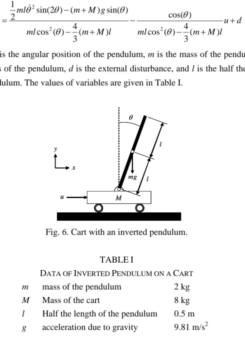
d u l M m ml l M m ml g M m ml + + − − + − + − = ) ( 3 4 ) ( cos ) cos( ) ( 3 4 ) ( cos ) sin( ) ( ) 2 sin( 2 1 2 2 2 θ θ θ θ θ θ θ&& & (45)
where θ is the angular position of the pendulum, m is the mass of the pendulum, M is the mass of the pendulum, d is the external disturbance, and l is the half the length of the pendulum. The values of variables are given in Table I.
y x l M mg u θ l y x l M mg u θ l
Fig. 6. Cart with an inverted pendulum.
TABLEI
DATA OF INVERTED PENDULUM ON A CART
m mass of the pendulum 2 kg
M Mass of the cart 8 kg
l Half the length of the pendulum 0.5 m
g acceleration due to gravity 9.81 m/s2
Assume the system is free of external disturbance and the reference signal θr(t) is
a sinusoid with the amplitude of π/30 in this example. The learning rates of weights are selected as η1=1.2 and η2 =1.0; the slope of tanh(⋅ at the origin is )
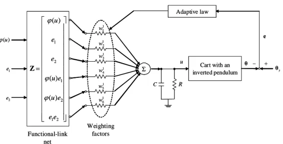
selected as a = 1.0. The resistance and capacitance are chosen as and . Solving the Riccati-like equation in (23) for a choice of and , we have . There exist two neurons and one control input for the HOHNN controller. The three inputs
Ω = 5 R F 005 . 0 = C Q 10= I
[
]
T c = 2 1 k ⎥ ⎦ ⎤ ⎢ ⎣ ⎡ = 5 5 5 15 P ) (uϕ , e1, and e2 are combined to form the
full input vector Z=
{
ϕ(u) e1 e2 ϕ(u)e1 ϕ(u)e2 e1e2}
which is fed into thethe following Fig. 7. Σ 1 3 w θ R C 1 2 w 1 4 w 1 5 w 1 1 w 1 6 w Cart with an inverted pendulum − y θ + e u Functional-link net ⎥ ⎥ ⎥ ⎥ ⎥ ⎥ ⎥ ⎥ ⎥ ⎥ ⎥ ⎥ ⎥ ⎥ ⎦ ⎤ ⎢ ⎢ ⎢ ⎢ ⎢ ⎢ ⎢ ⎢ ⎢ ⎢ ⎢ ⎢ ⎢ ⎢ ⎣ ⎡ = 2 1 2 1 2 1 ) ( ) ( ) ( e e e u e u e e u ϕ ϕ ϕ Z Adaptive law 1 e 2 e ) (u ϕ Weighting factors ΣΣ 1 3 w θ R C 1 2 w 1 4 w 1 5 w 1 1 w 1 6 w Cart with an inverted pendulum − y θ + e u Functional-link net ⎥ ⎥ ⎥ ⎥ ⎥ ⎥ ⎥ ⎥ ⎥ ⎥ ⎥ ⎥ ⎥ ⎥ ⎦ ⎤ ⎢ ⎢ ⎢ ⎢ ⎢ ⎢ ⎢ ⎢ ⎢ ⎢ ⎢ ⎢ ⎢ ⎢ ⎣ ⎡ = 2 1 2 1 2 1 ) ( ) ( ) ( e e e u e u e e u ϕ ϕ ϕ Z Adaptive law 1 e 2 e ) (u ϕ Weighting factors
Fig. 7. The overall diagram of cart with an inverted pendulum using HOHNN controller.
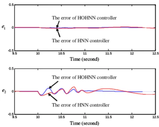
To compare the HNN controller, the simulation results for the proposed HOHNN and HNN controllers with external disturbance d=2.5sin(2t) when second are shown in Figs. 8-13. This fact shows the strong disturbance-tolerance ability of the proposed HOHNN controller. Figure 8 shows the reference signal
10 ≥ t ) (t r θ and the actual pendulum angle θ(t). The enlarging drawing of Fig. 8 from second to second is shown in Fig. 9. Figure 10 shows the comparison of errors using HNN and HOHNN controllers and their enlarging drawing are shown in Fig. 11. The mean squared errors using HNN and HOHNN controllers and their enlarging drawing are shown in Fig. 12 and 13. From the simulation results, the HOHNN controller can result in better acceptable tracking performance than HNN controller.
5 . 9 = t 5 . 12 = t 0 2 4 6 8 10 12 14 16 18 20 -0.2 0 0.2 0.4 0.6 0 2 4 6 8 10 12 14 16 18 20 -1 -0.5 0 0.5 1 1 x 2 x Time (second) Time (second) System performance using HNN controller System performance using HOHNN controller
Reference angular position
System performance using HNN controller
System performance using HOHNN controller Change of reference angular position
0 2 4 6 8 10 12 14 16 18 20 -0.2 0 0.2 0.4 0.6 0 2 4 6 8 10 12 14 16 18 20 -1 -0.5 0 0.5 1 1 x 2 x Time (second) Time (second) System performance using HNN controller System performance using HOHNN controller
Reference angular position
System performance using HNN controller
System performance using HOHNN controller Change of reference angular position
9.5 10 10.5 11 11.5 12 12.5 -0.5 0 0.5 9.5 10 10.5 11 11.5 12 12.5 -0.5 0 0.5 1 x 2 x Time (second) Time (second) System performance using HNN controller
System performance using HOHNN controller Reference angular position
System performance using HNN controller
System performance using HOHNN controller Change of reference angular position
2 e 1 e Time (second) Time (second) 0 2 4 6 8 10 12 14 16 18 20 -0.6 -0.4 -0.2 0 0.2 0 2 4 6 8 10 12 14 16 18 20 -1 -0.5 0 0.5 1
The error of HNN controller The error of HOHNN controller
The error of HNN controller The error of HOHNN controller
2 e 1 e Time (second) Time (second) 0 2 4 6 8 10 12 14 16 18 20 -0.6 -0.4 -0.2 0 0.2 0 2 4 6 8 10 12 14 16 18 20 -1 -0.5 0 0.5 1
The error of HNN controller The error of HOHNN controller
The error of HNN controller The error of HOHNN controller
9.5 10 10.5 11 11.5 12 12.5 -0.5 0 0.5 9.5 10 10.5 11 11.5 12 12.5 -0.5 0 0.5 2 e 1 e Time (second) Time (second) The error of HNN controller The error of HOHNN controller
The error of HNN controller The error of HOHNN controller
9.5 10 10.5 11 11.5 12 12.5 -0.5 0 0.5 9.5 10 10.5 11 11.5 12 12.5 -0.5 0 0.5 2 e 1 e Time (second) Time (second) The error of HNN controller The error of HOHNN controller
The error of HNN controller The error of HOHNN controller
Fig. 10. Comparison of errors using HNN and HOHNN controllers. Fig. 11. Detail of Fig. 10 from t = 9.5 second to t = 12.5 second.
0 2 4 6 8 10 12 14 16 18 20 0 0.5 1 1.5 2 2.5 Time (second)
Mean squared error of control system using HNN Mean squared error of control system using HOHNN
e 0 2 4 6 8 10 12 14 16 18 20 0 0.5 1 1.5 2 2.5 Time (second)
Mean squared error of control system using HNN Mean squared error of control system using HOHNN
e 9.5 10 10.5 11 11.5 12 12.5 0 0.05 0.1 0.15 0.2 0.25 0.3 0.35 0.4 0.45 0.5 Time (second) Mean squared error of
control system using HNN Mean squared error of control system using HOHNN
e 9.5 10 10.5 11 11.5 12 12.5 0 0.05 0.1 0.15 0.2 0.25 0.3 0.35 0.4 0.45 0.5 Time (second) Mean squared error of
control system using HNN Mean squared error of control system using HOHNN
e
Fig. 12. The mean squared errors using HNN and HOHNN controllers. Fig. 13. Detail of Fig. 12 from t=9.5 second to t=12.5 second.
6. Conclusion
This paper has proposed a high-order Hopfield-based neural network (HOHNN) controller for the nonlinear dynamical systems. The simulation shows that HOHNN is capable of controlling the behavior of dynamical systems and the weighting matrices in HOHNN can be found via Lyapunov criteria. The adaptive laws to tune the weighting matrix can reduce the error between practical and reference state. The simulation results for HNN and HOHNN are finally conducted to show that the performance of HOHNN controller is better than HNN controller even though the nonlinear dynamical system encounters a disturbance suddenly.
Reference
[1] J. J. Hopfield, “Neural networks and physical systems with emergent collective computational abilities,” Proceedings of National Academy of Sciences, USA, vol. 79, pp. 2554-2558, April 1982.
[2] Donq Liang, Lee, “Pattern Sequence Recognition Using a Time-Varying Hopfield Network,” IEEE Trans. Neural Networks, vol. 13, no. 2, pp. 330-342, March 2002.
[3] Pajares, “A Hopfiled Neural Network for Image Change Detection,” IEEE Trans. Neural Networks, vol. 17, no. 5, pp. 1250-1264, Sep. 2006.
[4] Y. H. Pao, Adaptive pattern Recognition and Neural Networks, Addison-Wesley,
Reading, 1989.
[5] Y. H. Pao, Functional-link net computing: theory, system architecture, and functionalities, Computer, 1992.
[6] Klassen, M. S. and Y. H. Pao, “Characteristics of the functional-link net: A higher order delta rule net,” IEEE Proceedings of 2nd Annual International Conference on Neural Networks, San Diago, CA, June 1995.
[7] Jagdish C. Patra, Ranendra N. Pal, B. N. Chatterji, and Ganapati Panda, “Identification of nonlinear dynamic systems using functional link artificial neural networks,” IEEE Trans. System, Man, and Cybernetics-part B:
Cybernetics, vol. 29, no. 2, pp. 254-262, April 1999.
[8] Simon Haykin, Neural Networks, Upper Saddle River, NJ: Prentice-Hall, 1999.
[9] L. X. Wang, Adaptive Fuzzy Systems and Control-Design and Stability Analysis,
Prentice-Hall, Englewood Cliffs, New Jersey, 1994.
[10] Y. G. Leu, W. Y. Wang, and T. T. Lee, “Observer-Based Direct Adaptive Fuzzy-Neural Control for Nonaffine Nonlinear Systems,” IEEE Trans. Neural
Networks, vol. 16, no. 4, pp. 853-861, 2005.
[11] S. H. Zak, Systems and Control, New York: Oxford Univ. Press, 2003.
[12] R. H. Cannon Jr., Dynamics of Physical Systems, New York: McGraw-Hill,
參加國際學術會議心得報告
王啟旭
國立交通大學電機系特聘教授, IEEE Fellow
2010 IEEE International Conference on Networking, Sensing and Control
The 2010 IEEE International Conference on Networking, Sensing and Control was held in Chicago, 10-13, April, USA. The main theme of the conference is technologies and applications for wireless sensory networks. In recent years, wireless sensory networks have opened several areas of research and applications. Many companies and research agencies have started working on the next generation of these networks. Wireless sensory networks are now used in many fields such as homeland security, agriculture, energy management, intelligent transportation and traffic engineering, logistics, warehouse management, disaster management, healthcare delivery, military, smart buildings, and manufacturing. This conference provides a remarkable opportunity for the academic and industrial community to address new challenges and share solutions, and discuss future research directions in the area of wireless sensory networks.
The purpose for me and my PhD student to participate in this conference is to present the major content in this NSC research project. The title of this paper is:
“Intelligent Adaptive Control of Uncertain Nonlinear Systems using Hopefield
Neural Networks”
This paper has also been submitted to IEEE Transactions on Control Systems Technology:, and is currently under minor revision. It is expected to be accepted by the end of 2010.
98 年度專題研究計畫研究成果彙整表
計畫主持人:王啟旭 計畫編號:98-2221-E-009-126-計畫名稱:動態類神經網路在非線性系統鑑別與控制器設計之應用 量化 成果項目 實際已達成 數(被接受 或已發表) 預期總達成 數(含實際已 達成數) 本計畫實 際貢獻百 分比 單位 備 註 ( 質 化 說 明:如 數 個 計 畫 共 同 成 果、成 果 列 為 該 期 刊 之 封 面 故 事 ... 等) 期刊論文 0 0 100% 研究報告/技術報告 0 0 100% 研討會論文 1 1 100% 篇 論文著作 專書 0 0 100% 申請中件數 0 0 100% 專利 已獲得件數 0 0 100% 件 件數 0 0 100% 件 技術移轉 權利金 0 0 100% 千元 碩士生 0 0 100% 博士生 0 0 100% 博士後研究員 0 0 100% 國內 參與計畫人力 (本國籍) 專任助理 0 0 100% 人次 期刊論文 0 0 100% 研究報告/技術報告 0 0 100% 研討會論文 0 0 100% 篇 論文著作 專書 0 0 100% 章/本 申請中件數 0 0 100% 專利 已獲得件數 0 0 100% 件 件數 0 0 100% 件 技術移轉 權利金 0 0 100% 千元 碩士生 2 0 100% 博士生 1 0 100% 博士後研究員 0 0 100% 國外 參與計畫人力 (外國籍) 專任助理 0 0 100% 人次其他成果