Adomian's decomposition method for electromagnetically induced transparency

(1)

Adomian’s decomposition method for electromagnetically induced transparency

Yee-Mou Kao*

Institute of Applied Mathematics, National Chiao Tung University, Hsinchu 300, Taiwan

T. F. Jiang

Institute of Physics, National Chiao Tung University, Hsinchu 300, Taiwan

Ite A. Yu

Department of Physics, National Tsing Hua University, Hsinchu 300, Taiwan

共Received 24 June 2005; published 6 December 2005兲

We developed the Adomian’s decomposition method to work for the electromagnetically induced transpar-ency 共EIT兲 problem. The method is general and capable to solve the coupled nonlinear partial differential equations for a light pulse passing through a three-level⌳-type coherent medium. This EIT system is described by the coupled Maxwell-Schrödinger equations and optical Bloch equations. In the weak probe field case, the results agree with perturbation solutions and experimental data. In the stronger probe field case while pertur-bation may fail, our results reproduce experimental data well. With the techniques of spatial and time parti-tions, we extend the decomposition method that will be versatile for the investigation of the light pulse propagating through a coherent atomic medium.

DOI:10.1103/PhysRevE.72.066703 PACS number共s兲: 02.70.Wz, 42.50.Gy, 03.65.Ge

I. INTRODUCTION

Recent progress for the control of light pulse propagations through a coherent medium inspires interesting discoveries. Namely, the electromagnetically induced transparency共EIT兲关1兴 and the frozen of light 关2兴 are two of the amazing phe-nomena. The technique to manipulate properties of light pulses关3兴 can be used to create large populations of coher-ently driven atoms. Types of optoelectronic devices关4兴 may be invented by this kind of technology. The basic principles involved in the two problems are delicate quantum interfer-ences. To our knowledge, except for the perturbational solu-tions, the general way of solutions to the system is still de-manding. We aim in this paper to develop a general tractable method to solve the related partial differential equations for the system. So, some realistic experimental physical param-eters are used and the results of the experiment and numeri-cal numeri-calculations are compared.

The method we developed here is the Adomian’s decom-position method共ADM兲. ADM solves nonlinear differential equations with decompositions; neither linearization nor per-turbation is necessary for the nonlinear part. The method has been widely applied to various domains in science and engi-neering. Adomian himself treated many physical topics such as the Navier-Stokes equations, Burger’s equation, the advection-diffusion equation, Korteweg–de Vries equation, nonlinear Schrödinger equation, etc.关5兴. ADM is extremely powerful for nonlinear physical problems, but no general treatments for eigenvalue problems are found. We recently developed a general ADM method for either linear or non-linear eigenvalue problems关6兴. Some of the techniques

de-veloped in the previous paper are adopted here, also. The ADM treatment of the quantum optical propagation problem is valuable to computational physics. It provides nonperturbative, semianalytical solutions. So the solution may be used to analyze the behaviors when the physical parameters change. This advantage is by no means beyond the capacity of usual numerical grids methods. Thus, the ADM method will enhance the understanding of EIT and related problems.

Consider a coherent medium consisting of ⌳-type three-level atoms with two metastable lower states兩1典, 兩2典, and an excited state 兩3典. In a typical experiment 关7兴, the medium contains one billion of ultracold87Rb atoms produced by a magneto-optical trap. The three states are chosen as hyper-fine levels of兩5S1/2, F = 1典, 兩5S1/2, F = 2典, and 兩5P3/2, F

⬘

= 2典. A weak probe pulse Ep共x,t兲=␧pe−i␻pt+ c . c. couples state 兩1典

and the excited state 兩3典, and a stronger control field

Ec共x,t兲=␧ce−i␻ct+ c . c. couples state兩2典 and state 兩3典, where

the pulse envelopes are slowly varying. Due to the long wavelength condition, the spatial dependence e±ikxof electric fields is neglected, however␧pand␧cstill depend on x.

The Maxwell-Schrödinger equations共MSE兲 with the Rabi frequencies ⍀p⬅d13␧p/ q and ⍀c⬅d23␧c/ q for the probe

field and control field are 1 c ⳵⍀p共x,t兲 ⳵t + ⳵⍀p共x,t兲 ⳵x = i␩Im关␳31兴, 共1兲 1 c ⳵⍀c共x,t兲 ⳵t + ⳵⍀c共x,t兲 ⳵x = i␩Im关␳32兴, 共2兲

where dijis the dipole-matrix element between states i and j,

␩= 3␭2_⌫N/共8_␲_{兲, and ⌫ is the spontaneous decay rate of the} excited state兩3典. The decay rates from 兩3典 to 兩1典 and to 兩2典 are usually assumed equal关8兴. N is the number density of the *Present address: Physics Division, National Center for

Theoret-ical Sciences, Hsinchu 300, Taiwan.

(2)

medium, and ␭ is the wavelength of the probe laser. We consider that the coupling frequency and the carrier fre-quency of the probe pulse are tuned resonantly. The density matrix elements␳ijare obtained from the optical Bloch

equa-tions共OBE兲 under the rotating-wave approximation 关9,10兴:

⳵␳11 ⳵t = ⌫ 2␳33− i⍀p 2 共␳13−␳31兲, ⳵␳22 ⳵t = ⌫ 2␳33− i⍀c 2 共␳23−␳32兲, 共3兲 and ⳵␳12 ⳵t = −␥␳12− i⍀c 2 ␳13+ i⍀p 2 ␳23, ⳵␳23 ⳵t = − ⌫ 2␳23− i⍀p 2 ␳21− i⍀c 2 共␳22−␳33兲, ⳵␳31 ⳵t = − ⌫ 2␳31+ i⍀c 2 ␳21+ i⍀p 2 共␳11−␳33兲, 共4兲 where␳ij are functions of x, and t and are complex in

gen-eral. In the OBE,␥ is the relaxation rate of the ground-state coherence. It can affect the amplitude of the output probe pulse significantly. The ␥ is a practical physical parameter but was usually neglected in other calculations. For example, in Ref. 关8兴 the authors calculate the problem nonperturba-tively. Merely, they did not consider the relaxation rate of ground-state coherence. In Ref. 关11兴, the authors treat the probe pulse as the perturbation, since they do not have the equations of populations. However, a constant population distribution is only valid for the perturbative calculation, i.e., the ground-state population of the probe field,␳11⬃1. Our goal is to solve the combined MSE and OBE by ADM with practical experimental parameters that may lie beyond the perturbative regime.

The paper is organized as follows. In Sec. II we introduce the scheme to decompose the spatial variable. In Sec. III we describe the decomposition of the time variable. In Sec. IV the time domain partition method is used to overcome the trouble of divergence in the series expansion of t. In Sec. V, for a stronger probe pulse case, we use the spatial domain partition method to resolve the convergent problem of x and present the results. Section VII is devoted to the concluding remarks.

II. DECOMPOSITION OF THE POSITION VARIABLE In the following, we denote the probability of the excited state as ␳e=␳33, and the reduced probability of the ground state as ␳g= 1 −␳11 for convenience. The conservation of probability requires ␳22=␳g−␳e. We find from Eq. 共4兲 that

␳12 is real and ␳23 and ␳31 are imaginary. We denote

␳12=␳␣, and␳23= i␳␤,␳31= i␳␥, where ␳e,␳g,␳␣,␳␤,␳␥,⍀c,

and ⍀p all are real functions. Thus the coupled MSE and

OBE become ⳵␳g ⳵t = − ⌫ 2␳e+⍀p␳␥, ⳵␳e ⳵t = −⌫␳e+⍀p␳␥−⍀c␳␤, ⳵␳␣ ⳵t = −␥␳␣− ⍀c 2 ␳␥− ⍀p 2 ␳␤, ⳵␳␤ ⳵t = − ⌫ 2␳␤− ⍀p 2 ␳␣− ⍀c 2 共␳g− 2␳e兲, ⳵␳␥ ⳵t = − ⌫ 2␳␥+ ⍀c 2 ␳␣+ ⍀p 2 共1 −␳g−␳e兲, 共5兲 and 1 c ⳵⍀p共x,t兲 ⳵t + ⳵⍀p共x,t兲 ⳵x = −␩␳␥, 共6兲 1 c ⳵⍀c共x,t兲 ⳵t + ⳵⍀c共x,t兲 ⳵x =␩␳␤. 共7兲

The ansatz of ADM is to expand the unknown solutions ⍀p共x,t兲, ⍀c共x,t兲, and␳i共x,t兲 in infinite series:

⍀p共x,t兲 =

兺

n=0 ⬁ ⍀p n_共t兲xn , ⍀c共x,t兲 =

兺

n=0 ⬁ ⍀c n_共t兲xn , ␳i共x,t兲 =

兺

n=0 ⬁ ␳i n_共t兲xn , 共8兲

where the superscript n designates the order of decomposi-tion. The initial conditions in this problem are

⍀p 0_{共t兲 = lim} t→0+ ⍀p共x = 0, t ⬎ 0兲, ⍀c 0_{共t兲 = ⍀} c共const兲, ␳i0共t = 0兲 =␳i共x = 0, t = 0兲 = 0. 共9兲

Let Lx represent ⳵/⳵x and Lt represent ⳵/⳵t. By the

as-sumption of Eq.共8兲, we rewrite the OBE in the form

Lt␳g0= − ⌫ 2␳e 0₊_⍀ p 0_␳ ␥ 0_, Lt␳e0= −⌫␳e0+⍀p0␳␥0−⍀c␳␤0, Lt␳␣0= −␥␳␣0− ⍀c 2 ␳␥ 0₋ ⍀p 0 2 ␳␤ 0_,

(3)

Lt␳_␤0= − ⌫ 2␳␤ 0₋⍀p 0 2 ␳␣ 0₊⍀c 2 共␳g 0_{− 2}_␳ e 0_兲, Lt␳_␥0= − ⌫ 2␳␥ 0 +⍀c 2 ␳␣ 0 +⍀p 0 2 共1 −␳g 0 −␳e 0_兲. _共10兲 By solving Eq.共10兲 with conditions of Eq. 共9兲, we can get

␳i

0_{共t兲. If we write Eqs. 共6兲 and 共7兲 in the form}

Lx⍀p= −␩␳␥− 1 cLt⍀p, 共11兲 Lx⍀c=␩␳␤− 1 cLt⍀c, 共12兲

and operate with the inverse operators Lx

−1 , we have ⍀p= −␩Lx −1_␳ ␥−1 cLx −1 Lt⍀p, 共13兲 ⍀c=␩Lx −1_␳ ␤− 1 cLx −1 Lt⍀c. 共14兲

By the assumption of Eq.共8兲, we get the ordinary differential equation ⍀p n+1_{共t兲 = −} 1 n + 1␩␳␥ n_{共t兲 −} 1 共n + 1兲cLt⍀p n_共t兲, _共15兲 ⍀cn+1共t兲 = 1 n + 1␩␳␤ n_{共t兲 −} 1 共n + 1兲cLt⍀c n_共t兲, _共16兲

where n艌0. Using ⍀p0共t兲, ⍀c0共t兲,␳i0共t兲 and Eqs. 共15兲 and 共16兲

we can get⍀_p1共t兲 and ⍀_c1共t兲.

For the higher orders of␳i, by Eq.共8兲 and the OBE, we

have Lt␳g n = −⌫ 2␳e n + Nx n_关⍀ p␳␥兴, Lt␳e n = −⌫␳e n + Nx n_关⍀ p␳␥兴 − Nx n_关⍀ c␳␤兴, Lt␳␣ n = −␥␳_␣n−1₂Nx n_关⍀ c␳␥兴 − 1 2Nx n_关⍀ p␳␤兴, Lt␳_␤n= − ⌫ 2␳␤ n −1 2Nx n_关⍀ p␳␣兴 − 1 2Nx n_关⍀ c␳g兴 − Nx n_关⍀ c␳e兴, Lt␳_␥ n = −⌫ 2␳␥ n +1 2Nx n_关⍀ c␳␣兴 + 1 2共⍀p n − Nx n_关⍀ p␳g兴 − Nx n_关⍀ p␳e兴兲, 共17兲 where the nonlinear function Nx

n_{关CD兴 is the nth order}

decom-position of function C共x,t兲 times D共x,t兲 with variable x; de-fined as Nx n_{关CD兴 ⬅} 1 n!

冋

冉

⳵ ⳵x

冊

n 关C共x,t兲 ⫻ D共x,t兲兴

册

x=0 . 共18兲 For example, if C共x,t兲=兺Cn_共t兲xm_{, and D共x,t兲=兺D}n_共t兲xm_,

then Nx1关CD兴=C0共t兲D1共t兲+C1共t兲D0共t兲.

In summary, our iteration procedure is to first apply the initial condition ⍀i

0_{共t兲 to Eq. 共10兲 and obtain} _␳

i

0_共t兲. Then from Eqs. 共15兲 and 共16兲 we obtain ⍀i1共t兲; the next

order ␳i1共t兲 is given through Eq. 共17兲, and so on.

Schematically: ⍀i 0_共t兲→_␳ i 0_{共t兲→⍀} i 1_共t兲→_␳ i 1_共t兲¯⍀ i k_共t兲→ ␳i k_共t兲

→⍀ik+1共t兲→␳ik+1共t兲¯ . We finally construct the functions

⍀i共x,t兲 and␳i共x,t兲 by Eq. 共8兲.

In the next section we show the method of solving differ-ential equations with variable t by ADM.

III. DECOMPOSITION OF THE TIME VARIABLE Expand the decomposition orders ⍀p

n_共t兲,⍀ c n_{共t兲, and} _␳ i n_共t兲 in series: ⍀p n_{共t兲 =}

兺

m=0 ⬁ ⍀p n,m tm, ⍀c n_{共t兲 =}

兺

m=0 ⬁ ⍀c n,m tm, ␳i n_{共t兲 =}

兺

m=0 ⬁ ␳i n,m tm, 共19兲

and with the initial conditions

冋

冉

d dt

冊

n 关E共t兲 ⫻ F共t兲兴

册

t=0 . 共24兲

For instance, if E共t兲=兺Em_tm_{and F共t兲=兺F}m_tm_{, then N} t

m=0

冉

m 共n + 1兲c⍀cn,m−1tm−1

冊

, 共26兲 or ⍀pn+1,m= − 1 n + 1␩␳␥ n,m₋ m + 1 共n + 1兲c⍀pn,m+1, 共27兲 ⍀cn+1,m= 1 n + 1␩␳␤ n,m₋ m + 1 共n + 1兲c⍀cn,m+1. 共28兲

With the initial conditions ␳_␥0,m,⍀p0,m and⍀c0,m, the next

order ⍀p

1,k

and ⍀c

1,k

for any k are derived from the above equation. Then⍀p1共t兲 and ⍀c1共t兲 can be derived. Similar

pro-cedures,⍀_pn共t兲 and ⍀_cn共t兲 for n艌2, can be found. To find higher orders␳i

, 共29兲

where the nonlinear function Nn,m_{关CD兴 is defined as the nth}

order in variable x and mth order in variable t of function

C共x,t兲; multiply D共x,t兲, Nn,m关CD兴 ⬅ Nt m_关N x n_关CD兴兴 = 1 n ! m!

冋

冉

⳵ ⳵x

冊

n

冉

⳵ ⳵t

冊

m 关C共x,t兲D共x,t兲兴

册

x=0,t=0 . 共30兲 For example, if C共x,t兲=兺Cn,m_xn_tm_{, and D共x,t兲=兺D}n,m_xn_tm_,

then N1,2_{关CD兴=共C}0,0_D1,2_{+ C}0,1_D1,1_{+ C}0,2_D1,0_兲+共C1,0_D0,2 + C1,1_D0,1_{+ C}1,2_D0,0_兲.

We now already have enough information to obtain all the functions. For a known⍀p

k_{共t兲 and ⍀} c

k_{共t兲, our procedure starts}

from the initial condition ␳ik,0, then proceeds schematically

␳i k,0_→_␳ i k,1_{→ ¯ →}_␳ i k,m

, . . . , to construct the functions ␳i k_共t兲.

We use␳_␥k,m and⍀pk,m+1 to obtain ⍀k+1,mp , and use ␳␤k,m and

⍀c k,m+1

to obtain⍀c k+1,m

, to construct the higher decomposi-tion funcdecomposi-tion⍀pk+1共t兲 and ⍀ck+1共t兲.

Combine the decomposition x and t method, all the func-tions ⍀i共x,t兲 and ␳i共x,t兲, and hence the solution to the

coupled equations are obtained.

IV. THE TIME DOMAIN PARTITION METHOD To justify the convergence of series expansion of t, we divide the time domain 关0,T兴 into a union of q partitions 关Tm−1, Tm兴, m=1,2,3, ... ,q. And the electric field function

⍀i

n_{共t兲 and density functions} _␳ i

n_{共t兲 in the mth partition are}

denoted as⍀_i,mn 共t兲 and␳_i,mn 共t兲 with t苸关Tm−1, Tm兴. The global

(5)

⍀i n_{共t兲 =}

兺

m=1 q ⍀i,m n _共t兲_␹ m共t兲, ␳i n_{共t兲 =}

兺

m=1 q ␳i,m n _共t兲 ␹m共t兲, t苸关0,T兴, 共31兲 where ␹m共t兲 =

再

1, t苸关Tm−1,Tm兴, 0, t⫽ 关Tm−1,Tm兴, 共32兲 and 关0,T兴 = 艛 m=1 q 关Tm−1,Tm兴. 共33兲

We reset the connection conditions at t = Tmas

⍀i,m n _共⌬ mT兲 = ⍀i,m+1 n _共0兲, ␳i,m n _共⌬ mT兲 =␳i,m+1 n _共0兲, _共34兲

where⌬mT = Tm− Tm−1is the length of the interval关Tm−1, Tm兴.

With this partition method, we overcome the problem of con-vergence in time domain. The method was developed in our previous treatment of ADM eigenvalue problems关6兴.

In the following, we consider a Gaussian temporal pulse passing through the coherent medium. The initial condition of the field is ⍀0p共t ⬎ 0兲 = ⍀0exp

冋

−

冉

t − t0

冑

2␶

冊

2

册

, 共35兲 ⍀c 0_{共t兲 = ⍀} c. 共36兲

Our first example is a weaker field case so that we can compare the results with perturbation theory. We take ⍀0 = 0.01⌫,t0= 3␶,␶= 240/⌫,␥= 0.001⌫, and ␩= 9.06⌫/L, where L is the length of the medium. Here L = 780␮m, and ⌫=3.77⫻107_{/ sec;} _⍀

c= 0.3⌫ is the Rabi frequency of the

coupling laser.

Notice that the reset initial condition for each interval is ⍀p,m 0 _{共t兲 = ⍀} p 0_共T m−1+ t兲 =⍀0e−关共Tm−1+ t − t0兲/冑2␶兴2_, _t苸关0,⌬ mT兴. 共37兲

We choose T = 6␶, and slice the time domain into

q = 24 000 parts. The choice of the number q is related to the

size of time slice⌬mT. Assume the machine accuracy of a

numerical computation is⑀, then after propagation of q steps, the accumulative error is estimated to be O共q⫻⑀兲. Thus, the smaller value of q provides higher accuracy than larger value of q. On the other hand, smaller q means larger value of ⌬mT. To reach the expected accuracy, the ADM expansion

must go to higher order. For nonlinear PDE, higher order terms are complicated. The compromise is to choose a larger value of q and keep modest order in expansion so that proper accuracy can be obtained. If the accuracy criterion is set to

O共10−10_{兲, and}_⑀_{= 10}−16_{, we need q}_艋O共106_兲.

In Fig. 1, we depict the results of⍀p共x,t兲 in Eq. 共8兲 and

its associated decompositions up to the sixth order at the end

point of medium x = L. Note that⍀0_pis the input pulse at the beginning end x = 0. The peak ratio of ⍀p共x=0,t兲 to

⍀p共x=L,t兲 agrees with the spatial variation from the

pertur-bational theory and will be discussed later. We can also see that the magnitude decreases from order to order and the magnitude of the sixth order is negligibly small. Thus, the convergence in expansion orders is justified. Figure 2 shows the time evolutional results of states probabilities and the coherence at the end x = L. During the calculation, the spatial domain expansion order is 6 and the time domain expansion order is 4. The numerical error in time is less than 10−9_{, and} is less than 10−3_{in spatial expansion.}

A. The perturbation theory

In the previous calculation, the amplitude of control field ⍀chas the same order of magnitude of⌫ and is 30 times of

FIG. 1. 共Color online兲 The probe field in Eq. 共8兲. The curve Input denotes the probe pulse at the beginning end x = 0, and the curve Output is at the end of medium x = L. Also shown are decom-position orders. The labels⍀n_{are shorthand for}_⍀

p

n_{in Eq.}_{共8兲. The}

parameters are ⍀0= 0.01⌫, ⍀c= 0.3⌫, ␶=240/⌫, ␥=0.001⌫, and

␩= 9.06⌫/L.

FIG. 2.共Color online兲 The density functions␳i共t兲 as functions of

time at the end of medium x = L. Also shown are␳_i0共t兲 at the begin-ning end x = 0. The parameters are the same as Fig. 1. The meabegin-nings of indices are described in the text.

(6)

the probe pulse⍀p. We have⍀pⰆ⍀c,⌫. Due to the optical

pumping effect by the strong control field, all population is nearly in the兩1典 state and, hence,␳g,␳eⰆ1. The optical

co-herence is qualitatively proportional to the Rabi frequency of the driving field multiplied by the ground-state population. The population in the兩1典 state is driven by the very weak ⍀p and the negligible␳g is driven by the control field. It is

reasonable that␳_␤,␳_␥Ⰶ␳_␣and the change rates of␳_␤and␳_␥ are much smaller than⍀cand⌫. Under the above conditions,

we neglect the term of⍀p␳␤/ 2 in the third equation of Eq.

共5兲; 1−␳g−␳e⬇1 and the terms of ⳵␳␥/⳵t and ⌫␳␥/ 2 are

negligible in the fifth equation of Eq.共5兲. We then have

⳵␳␣ ⳵t ⯝ −␥␳␣− ⍀c 2 ␳␥, 0⯝⍀c 2 ␳␣+ ⍀p 2 . 共38兲

By using the results of Eq.共38兲 and the condition that ⍀cis

a constant, we obtain ␳␥⯝ _⍀2 c 2 ⳵⍀p ⳵t + 2␥ ⍀c2 ⍀p. 共39兲

Plug this expression ␳_␥ into MSE of Eq. 共6兲, the traveling wave equation becomes

冉

1 c+ 2␩ ⍀c2

冊

⳵⍀p共x,t兲 ⳵t + ⳵⍀p共x,t兲 ⳵x = − 2␥␩ ⍀c2 ⍀p, 共40兲

so we find that the group velocityvg satisfies

1 vg =1 c+ 2␩ ⍀c2 . 共41兲

The amplitude as a function of the position is ⍀p共x,t兲 = ⍀p共t兲exp

冉

−

2␥␩x

⍀c

2

冊

. 共42兲

B. The comparison of ADM and perturbational results If 2␩/⍀c2Ⰷ1/c, with the physical parameters described

above, we then have

vg⯝

⍀c2

2␩= 145.9 m/s. 共43兲

The traveling time of the pulse through the medium is L /vg,

in the dimensionless unit

r⌬t = L vg

= 201.5. 共44兲

At x = L, the decay factor is

exp共−␥⌬t兲 = exp共− 0.202兲 = 0.817. 共45兲 From the ADM data presented in Fig. 1, the decay in the peak heights of the probe pulse at the input and output posi-tion 共curves labeled with Input and Output兲, agrees quite

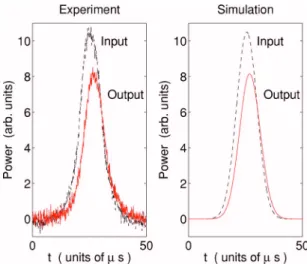
well with the perturbation formula of Eq. 共45兲. Our ADM results also reproduce the experimental data as shown in Fig. 3 with parameters described in the captions of that figure.

V. THE SPATIAL DOMAIN PARTITION METHOD In the next simulation, we increase the light pulse ampli-tude but reduce the width of the pulse, so that the perturba-tion theory may not work. The direct use of the same ADM as described previously is divergent in spatial series. To guar-antee the convergence of series expansion in x, we divide the domain 关0,X兴 into r partitions 关X_m−1, Xm兴, m=1,2,3, ... ,r,

just like the method we developed for the nonlinear eigen-value problem of the Gross-Pitaevskii equation 关6兴. So the field function⍀i共x,t兲 and density functions␳i共x,t兲 in the mth

partition are denoted as ⍀i,m共x,t兲 and ␳i,m共x,t兲 with

t苸关Tm−1, Tm兴. The global solutions are given by

⍀i共x,t兲 =

兺

m=1 q ⍀i,m共x,t兲␹m共x兲, ␳i共x,t兲 =

兺

m=1 q ␳i,m共x,t兲␹m共x兲, x苸关0,X兴, 共46兲 where ␹m共x兲 =

再

1, x苸关X_m−1,Xm兴, 0, x⫽ 关Xm−1,Xm兴, 共47兲 and 关0,X兴 = 艛 m=1 r 关Xm−1,Xm兴. 共48兲

The connection conditions at x = Xmare

FIG. 3.共Color online兲 The comparison of the experimental data and numerical simulation. ⍀_c= 0.35± 0.03⌫, ⍀₀= 0.07± 0.01⌫, ␩= 3.6± 0.2⌫/L, ␥=共3±1兲⫻10−3⌫, and ␶=240/⌫ are determined experimentally 关7兴. ⍀c= 0.35⌫, ⍀0= 0.07⌫, ␩= 3.6⌫/L, ␥=2⫻10−3_{⌫, and}_{␶=240/⌫ are used in the calculation.}

(7)

⍀i,m共⌬mX,t兲 = ⍀i,m+1共0,t兲,

␳i,m共⌬mX,t兲 =␳i,m+1共0,t兲, 共49兲

where ⌬mX = Xm− Xm−1 is the length of the interval

关Xm−1, Xm兴. With the spatial partition method, the

conver-gence problem in the series expansion of the spatial domain is resolved. With the above condition for light pulse, we divide the space into ten partitions and solve the coupled OBE and MSE by ADM. We show in Fig. 4 the time evolu-tions of a Gaussian pulse passing through a medium of ⌳-type three-level atoms at various positions in the medium. In the simulation,⍀0 is 0.1⌫ which is ten times larger than the case in Fig. 1, and with much shorter width ␶= 28/⌫. Interestingly, we find that the stronger and narrower light pulse is now more diffused by the medium than the case in the previous section. Experiments show that the EIT fre-quency transmission window is narrower compared to the previous parameter set of a weaker field case. The narrower

frequency band transmitted causes the pulse shape to be broader in the time domain. This phenomenon has not been explained by the perturbation calculation.

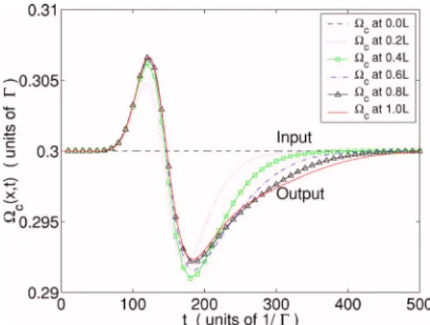
Figure 5 depicts the time evolutions of the control field at several places in the medium. At the beginning end共x=0兲, the field is fixed at the level of 0.3. The limiting case with

␥= 0 was shown in关8兴. Our results take␥into consideration;

␥ can affect the amplitude of output probe pulses signifi-cantly. The behavior of the output probe pulse in the medium is quite different from those calculated with␥= 0. To exhibit the effect of␥, we show in Fig. 6 the results of␥= 0, 0.001, and 0.002⌫ and the other parameters are set equal to those of Fig. 1. The output probe pulse amplitude of the case with nonvanishing ␥ is significantly lower than the case with

␥= 0.

Figure 7 shows the comparisons between calculation and experimental results in real time. Significantly different from the case shown in Fig. 3, the output probe pulse is broadened FIG. 4.共Color online兲 The pulse shape of fields passing through

a medium of⌳-type three-level atoms at various places in the me-dium. ⍀_p are shorthand for ⍀_p共x,t兲 at labeled positions. The parameters are ⍀0= 0.1⌫, ⍀c= 0.3⌫, ␶=28/⌫, ␥=0.001⌫, and

␩= 9.06⌫/L.

FIG. 5.共Color online兲 The time evolutions of the control field at several places in the medium of⌳-type three-level system. ⍀care

shorthand for⍀_c共x,t兲 at labeled positions. The parameters are the same as Fig. 3.

FIG. 6. 共Color online兲 The input ⍀c 共x=0,t兲 and output probe

pulses⍀_c共x=L,t兲 at␥=0, 0.001, and 0.002⌫. The other parameters are equal to those of Fig. 1.

FIG. 7.共Color online兲 The comparison of the experimental data and numerical simulation. ⍀_c= 0.30± 0.03⌫, ⍀₀= 0.10± 0.01⌫, ␩= 3.6± 0.2⌫/L, ␥=共3±1兲⫻10−3⌫, and ␶=28/⌫ are determined experimentally 关7兴. The experimental data are taken through a 20-MHz low-pass filter. ⍀_c= 0.33⌫, ⍀₀= 0.10⌫, ␩= 3.6⌫/L, ␥=2⫻10−3_{⌫, and}_{␶=28/⌫ are used in the calculation.}

(8)

and asymmetrical with a longer tail. The agreement between the experimental data and the theoretical prediction is satis-factory. The agreements in both weak and stronger field cases are excellent. This justifies that our ADM method works well for either perturbative or nonperturbative cases.

VI. CONCLUSION

We show the Adomian’s decomposition method can pro-vide semianalytical solutions for the problems of light pulse passing through a medium of⌳-type three-level atoms. Un-like other numerical grids methods, the ADM technique gives explicit forms of solution. The direct use of the power series expansion method 共or modified decomposition method兲 may not be able to solve the partial differential equation straightforwardly. In that case, the spatial partition method is a recipe to provide convergent results.

In summary, we have developed in this paper a new and efficient algorithm to solve the coupled partial differential equations of MSE and OBE for the three-level EIT problem. All the computations reported here are carried out on a per-sonal computer. The four levels are related to the problems; such as photon switching by quantum interference关12兴. It is far more complicated than the three-level system but is in-teresting. The method of the solution is currently under de-velopment and will be reported in the future.

ACKNOWLEDGMENTS

We thank the authors of Ref.关7兴 for providing the experi-mental data for direct comparison with our theoretical inves-tigations. TFJ acknowledges the support from the National Science Council of Taiwan under Contract No. NSC93-2112-M009-024.

关1兴 A. Kasapi, M. Jain, G. Y. Yin, and S. E. Harris, Phys. Rev. Lett. 74, 2447共1995兲.

关2兴 L. V. Hau, S. E. Harris, Z. Dutton, and C. H. Behroozi, Nature 共London兲 397, 594 共1999兲; C. Liu, Z. Dutton, C. H. Behroozi, and L. V. Hau, ibid. 409, 490共2001兲; M. Bajcsy, A. S. Zibrov, and M. D. Lukin, ibid. 426, 638共2003兲.

关3兴 M. D. Lukin and A. Imamoglu, Nature 共London兲 413, 273 共2001兲; M. Fleischhauer and M. D. Lukin, Phys. Rev. Lett. 84, 5094共2000兲.

关4兴 S. E. Harris, Phys. Today 50共7兲, 36 共1997兲.

关5兴 G. Adomian, Solving Frontier Problems of Physics: The

De-composition Method共Kluwer, Dordrecht, 1994兲.

关6兴 Y. M. Kao and T. F. Jiang, Phys. Rev. E 71, 036702 共2005兲. 关7兴 Y. F. Chen, Z. H. Tsai, Y. C. Liu, and Ite A. Yu, Opt. Lett. 共to

be published兲.

关8兴 T. N. Dey and G. S. Agarwal, Phys. Rev. A 67, 033813 共2003兲. 关9兴 M. O. Scully and M. S. Zubairy, Quantum Optics 共Cambridge

University Press, Cambridge, UK, 1997兲.

关10兴 S. Alam, Lasers without Inversion and Electromagnetically

In-duced Transparency共SPIE, Washington, 1999兲.

关11兴 A. K. Patnaik, F. L. Kien, and K. Hakuta, Phys. Rev. A 69, 035803共2004兲.

关12兴 S. E. Harris and Y. Yamamoto, Phys. Rev. Lett. 81, 3611 共1998兲.