Spin-Hall interface resistance in terms of Landauer-type spin dipoles
A. G. Mal’shukov,1L. Y. Wang,2and C. S. Chu21Institute of Spectroscopy, Russian Academy of Science, 142190 Troitsk, Moscow oblast, Russia 2Department of Electrophysics, National Chiao Tung University, Hsinchu 30010, Taiwan
共Received 9 November 2006; published 12 February 2007兲
We considered the nonequilibrium spin dipoles induced around spin-independent elastic scatterers by the intrinsic spin-Hall effect associated with the Rashba spin-orbit coupling. The spin polarization normal to the two-dimensional electron gas共2DEG兲 has been calculated in the diffusion range around the scatterer. Although around each impurity this polarization is finite, we found that the corresponding macroscopic spin density obtained via averaging of individual spin dipole distributions over impurity positions is zero in the bulk. At the same time, the spin density is finite near the boundary of 2DEG, except for a special case of a hard wall boundary, that is, when it turns to 0. The boundary value of the spin polarization can be associated with the interface spin-Hall resistance determining the additional energy dissipation due to spin accumulation. DOI:10.1103/PhysRevB.75.085315 PACS number共s兲: 73.40.Lq, 72.25.Dc, 71.70.Ej
I. INTRODUCTION
Most of the theoretical studies on the spin-Hall effect 共SHE兲 have been devoted to the calculation of the spin cur-rent 共for a review, see Ref. 1兲. Such a current is a linear response to the external electric field E, which induces a spin flux of electrons or holes flowing in the direction perpendicu-lar to E. This spin flux can be due either to the intrinsic spin-orbit interaction共SOI兲 inherent to a crystalline solid2or
to the spin-dependent scattering from impurities.3The
spin-Hall current, as a response to the electric field, is character-ized by the spin-Hall conductivity. On the other hand, similar to the conventional Hall effect, one can introduce the spin-Hall resistivity to the calculation of the local chemical po-tential differences=↑−↓ as a response to the dc electric
current. For the two-dimensional electron gas共2DEG兲 in a local equilibrium, this potential difference can be related to the z-component共perpendicular to 2DEG兲 of the spin polar-ization according to Sz= NFs, where NF is the density of
states near the Fermi level. Therefore, the spin-Hall resistiv-ity is closely associated with spin accumulation near the in-terfaces. It should be noted that measuring spin polarization is thus far the only realistic way to detect SHE.4,5For
inter-faces of various types, such an accumulation has been calcu-lated in a number of works.6–12A typical example to study
spin accumulation is an infinite 2D strip along the x-direction with a width w along the y-direction. In this geometry, the dc flows in the x-direction while the spin-Hall current flows in the y-direction, with the spin density accumulating near the boundaries. An analog of the Hall voltage could be a differ-ence ofs on both sides of the strip. There is, however, a
fundamental distinction from the charge Hall effect. In the latter case, due to the long-range nature of the electric poten-tial created by conserving electric charges, the Hall voltage is proportional to the width of the strip. In contrast, the spin-Hall electrochemical potential at the interface does not de-pend on w as w→⬁ because spin relaxation essentially sup-presses the long-range contribution to spin-polarization buildup near the interfaces. Hence, it is sensible to introduce an interface spin-Hall resistance, which is the proportionality coefficient between the interface value ofsand the electric
current density.
Below, we will consider the spin-Hall resistance from the microscopic point of view. This approach is based on
Landauer’s13idea that at a given electric current, each
impu-rity is surrounded by a nonequilibrium charge cloud forming a dipole. Combined together, these dipoles create a voltage drop across the sample. Therefore, each impurity plays a role of an elementary resistor. In a similar way, nonequilibrium spin dipoles could be induced subsequent to the spin-Hall current. One may expect that the spin cloud will appear around a spin-orbit scatterer in the case of an extrinsic SHE, as well as around a spin-independent scatterer in the case of the intrinsic effect. The latter possibility for a 2D electron gas with Rashba interaction has been considered in Ref.14. The polarization perpendicular to 2DEG was calculated within the ballistic range around a scatterer. On the other hand, in order to study spin accumulation and the spin-Hall resistance on a macroscopic scale, one needs to calculate the spin-density distribution at distances much larger than the mean free path l of electrons. Below, we will extend the Green’s function method of Ref.14to the diffusive range. In Sec. II, the spin-density distribution around an individual target impurity will be calculated. In Sec. III, we will con-sider the interface spin accumulation created by spin dipoles randomly but homogeneously distributed in space. A relation between spin-Hall resistance and energy dissipation will be discussed in Sec. IV. A summary and discussion of results will be presented in Sec. V.
II. SPIN CLOUD INDUCED BY A SINGLE IMPURITY It is known that the electric field applied to a homoge-neous 2DEG with the Rashba SOI induces a component of the nonequilibrium spin polarization parallel to 2DEG.15The spin-Hall effect produces, however, a zero-spin polarization in its z-component. This understanding about such a
homo-geneous gas has implied an averaging over impurity
posi-tions. An impure system, on the other hand, cannot be uni-form on a microscopic scale. The effect of each impurity on the spin polarization could be singled out by considering an impurity共a target impurity兲 at a fixed position while taking at the same time the average over positions of other impurities. In such a way, the Landauer electric dipole has been calculated.16,17The electron density around a target impurity
represented by the elastic scatterer was found from the
asymptotic expansion of the scattered wave functions of the electrons. At the same time, the wave vectors of incident particles were weighted with the nonequilibrium part of the Boltzmann distribution function. We will employ another method based on the Green’s function formalism.14 Within
this method, the spin-density response to the electric field E is given by the standard Kubo formula, with the scattering potential of the target impurity incorporated into the retarded and advanced Green’s functions Gr/a共r,r
⬘
,兲 denoted by the superscripts r and a, respectively. As such, the n-component of the stationary spin polarization is given bySn共r兲 = − e m*
冕
d 2r⬘
冕
d 2 dnF共兲 d ⫻ Tr关n Gr共r,r⬘
,兲共vE兲Ga共r⬘
,r,兲兴, 共1兲 where the overbar denotes averaging over impurity positions, the trace runs through the spin variables, and nF共兲 is theFermi distribution function. To avoid further confusion, we note that the angular moment is obtained by multiplying
Sn共r兲 by ប/2 and e is the particle charge, which is negative
for electrons. At low temperatures, only in close vicinity around EF contributes to the integral in Eq. 共1兲. Therefore,
below we set = EF and omit the frequency argument in
Green’s functions. Further, v is the particle velocity operator containing a spin-dependent part associated with SOI. Writ-ing SOI in the form
Hso= hk·, 共2兲
one obtains the velocity operator
vj= k
j m*+
hk·
kj , 共3兲
where⬅共x,y,z兲 is the Pauli matrix vector. In the case
of the Rashba interaction, the spin-orbit field hkis given by
hx=␣ky, hy= −␣kx. 共4兲
We assume that the target impurity, located at ri, is
repre-sented by a scattering potential U共r−ri兲. The Green’s
func-tions in Eq.共1兲 have to be expanded in terms of this poten-tial. Up to the second order in U, one obtains
Gr/a共r,r
⬘
兲 = Gr/a共0兲共r,r⬘
兲 +冕
ds2Gr/a共0兲共r,s兲U共s − ri兲⫻Gr/a共0兲共s,r
⬘
兲 +冕
ds2ds⬘
2Gr/a共0兲共r,s兲U共s − r i兲⫻Gr/a共0兲共s,s
⬘
兲U共s⬘
− ri兲Gr/a共0兲共s
⬘
,r⬘
兲. 共5兲The unperturbed functions Gr/a共0兲 depend, nevertheless, on the scattering from background random impurities. The latter create the random potential Vsc共r兲, which is assumed to be
delta correlated, so that the pair correlator 具Vsc共r兲Vsc共r
⬘
兲典=⌫␦共r−r
⬘
兲/NF, where⌫=1/2is expressed via the meanelastic scattering time. The delta correlation means that the corresponding impurity potential is the short-range one. In fact, the potential of the target impurity could be different from that of the random impurities. It might be a special sort
of impurities added to the system. On the other hand, the target and the random impurities would be identical if one would try to employ the spin dipoles for the interpretation of spin accumulation near interfaces.
After the substitution of Eq. 共5兲 into Eq. 共1兲, one must calculate the background impurity configurational averages containing the products of several Green’s functions G共0兲. Assuming that the semiclassical approximation EFⰇ1 is
valid, the standard perturbation theory18,19can be employed.
Its whose building blocks are the so-called ladder perturba-tion series expressed in terms of the unperturbed average Green’s functions
Gkr/a=
冕
d2共r − r⬘
兲eik共r−r⬘兲Gr/a共0兲共r,r⬘
兲 共6兲given by the 2⫻2 matrix,
Gk
r/a
=共EF− Ek− hk·± i⌫兲−1, 共7兲
where Ek= k2/共2m*兲. When averaging the Green’s function
products within the ladder approximation, only pairs of re-tarded and advanced functions carrying close enough mo-menta should be chosen to become elements of the ladder series. After decoupling the mean products of Green’s func-tions into the ladder series, the Fourier expansion of Eq.共1兲 can be represented by the diagrams shown in Fig.1. In these diagrams, the diffusion ladder renormalizes both the left-hand and right-left-hand vertices. The renormalized left-left-hand vertex⌺z共q兲 is associated with the qth Fourier component of
the induced spin density, and the corresponding diffusion propagator enters with the wave vector q. In its turn, the right-hand vertex T共p兲 related to the homogeneous electric field is represented by the ladder at the zeroth wave vector. The corresponding physical process is the D’yakonov-Perel’20 spin relaxation of a uniform spin
distri-bution. This left-hand vertex alone contributed to the ballistic case result,14while⌺z共q兲 has been taken unrenormalized due
to large values of qⰇ1/共vF兲1 in the ballistic regime.
Fig-ures1共e兲and1共f兲represent some diagrams where the diffu-FIG. 1. Examples of diagrams for the spin density. Scattering of electrons by a target impurity is shown by the solid circles. Dashed lines denote the ladder series of particle scattering by the random potential. p,k, and k⬘are the electron momenta.
sion process separates two scattering events. As will be shown below, such diagrams give rise to small corrections to the spin density and can be neglected. Hence, the main con-tribution comes from the diagrams similar to those in Figs. 1共a兲–1共d兲. The corresponding spin polarization has the form
Sz共q兲 = 1 2
兺
p,k Tr关Gpk a ⌺ z共q兲Gk+q,p r T共p兲兴. 共8兲The functions Gkr/a⬘kare formally represented by the Fourier expansion of Eq.共5兲 with respect to r and r
⬘
, provided that the respective average values G共0兲共r,r⬘
兲, instead of G共0兲共r,r⬘
兲, are substituted. Evaluating the pair products ofsuch functions in Eq.共8兲, one should take into account only the terms up to the second order with respect to the scattering potential U.
The vertices⌺z共q兲 and T共p兲 can be easily calculated. As
was discussed in Ref.14, due to considerable cancellation of the diagrams which is known from literature on the spin-Hall effect, T共p兲 acquires a quite simple form in a special case of the Rashba SOI. Namely,
T共p兲 = e
m*p · E. 共9兲
In its turn,⌺z共q兲 is expressed in terms of the diffusion
propa-gator. Indeed, let us represent this vertex using a basis of four 2⫻2 matrices0= 1 and i=i, with i = x , y , z. Then, ⌺z共q兲
can be written as ⌺z共q兲 =
兺
b
Dzb共q兲b, b = 0,x,y,z, 共10兲
where Dzb共q兲 are the matrix elements of the diffusion
propa-gator satisfying the spin-diffusion equation, as it was de-scribed in Ref. 6 and references therein. The nondiagonal element Dz0共q兲 appears due to the spin-charge mixing and it is zero for SOI of a quite general form, including the Rashba interaction.21–24 Finally, from Eq. 共8兲, using Eqs. 共9兲 and
共10兲, we express Sz共q兲 in the form Sz共q兲 =
兺
n=x,y,z Dzn共q兲In共q兲, 共11兲 where In共q兲 = e 2m*兺
p,k共p · E兲Tr关Gpk a nG k+q,p r 兴. 共12兲The function In共q兲 has a simple physical meaning. For n
= x , y , z, it represents a source of spin-polarized particles emitting from the target impurity. Their further diffusion and spin relaxation result in the observable polarization. This source term feature is conceptually similar, though different in its context, to the original charge cloud consideration when SOI is not present and the Boltzmann equation is used to describe the subsequent background scattering.13,16 For q
Ⰶl−1Ⰶk
F, the source can be expanded in powers of q.
Therefore, the wave-vector-independent terms represent the delta source located at ri, while the terms linear in q are
associated with the gradient of the delta function. Below, we will keep only the constant and linear terms for each nth
component In共q兲 and assume, for simplicity, the short-range
scattering potential U共r兲, so that its kth Fourier transform is simply U exp共−ik·ri兲, where U is a constant. Further, In共q兲
can be written as
In共q兲 = I1n共q兲 + I2n共q兲, 共13兲
where I1 and I2 are of the first and the second order with respect to the scattering potential U, respectively. Accord-ingly, I1 and I2 are represented by Figs. 1共a兲and 1共b兲 and Figs. 1共c兲 and 1共d兲, respectively. Using Eq. 共5兲 to express Green’s functions Gkr/a⬘kin Eq.共12兲, we obtain
I1n共q兲 = eU 2m*e iq·ri
兺
p 共p · E兲Tr关Gp r Gp a共 n Gp+qr + Gp−qa n兲兴 共14兲 and I2 n共q兲 = eU2 2m*e iq·ri兺
pk 共p · E兲Tr关Gp r Gp a共G k a n Gk+qr −␥nGp+qr +␥Gp−qa n兲兴, 共15兲 where ␥= i Im冉
兺
k Gk a冊
= iNF. 共16兲In our following consideration, we let the x-axis be parallel with the electric field and the z-axis be perpendicular to the 2DEG. The system Hamiltonian is symmetric under a sym-metry operation combining a reflection from the plane per-pendicular to the y-axis, that is, py→−py, and a unitary
transformationi→
yiy. Applying this transformation to
Eq. 共12兲, one can easily see that Ix共q
x, qy兲=−Ix共qx, −qy兲, Iz共q
x, qy兲=−Iz共qx, −qy兲, and Iy共qx, qy兲=Iy共qx, −qy兲. Making
use of another symmetry operation px→−px, py→−py, and i→
ziz, we obtain Ix共qx, qy兲=Ix共−qx, −qy兲, Iz共qx, qy兲=
−Iz共−qx, −qy兲, and Iy共qx, qy兲=Iy共−qx, −qy兲. From these
rela-tions, it is easy to see that the expansion of Iz into a power series starts from linear in q terms, while the leading term in
Iyis constant and the next one is quadratic in q. Because of
this reason, only the constant will be taken into account in Iy.
The expansion of Ixstarts from qxqy, and this source
compo-nent will be neglected.
The calculation of I1and I2given by Eqs.共14兲 and 共15兲 is based on the standard linearization near the Fermi level, thus ignoring band effects giving rise to small corrections ⬃hkF/ EF and⌫/EF. Further, the diffusion approximation is
valid at qⰆ1/l. At the same time, the characteristic length scale is determined by the spin-relaxation length lso, which is the distance a particle diffuses during the D’yakonov-Perel’ spin-relaxation timeso= 4共hk
F
2兲−1. The corresponding diffu-sion length lso=
冑
Dso, where D =vF2
/ 2 is the diffusion con-stant. Hence, lso=vF/ hkF. Taking q⬃1/lso, one finds that the diffusion approximation is valid if hkF/⌫Ⰶ1. Therefore,
within this approximation, we will retain only the leading powers of hkF/⌫Ⰶ1. In such a way, direct calculation of I1
with Green’s functions and SOI given by Eqs. 共7兲 and 共4兲, respectively, shows that both I1y and I1z are small by a factor of⌫/EF. For example, using the relation
共Gkr/a兲2= −
EF
Gkr/a, 共17兲
which follows from Eq.共7兲, evaluating I1y at q = 0, one can represent the corresponding sum in Eq.共14兲 as
− EF
兺
p pxTr关Gp r Gp a y兴 = − EF冉
2 ⌫ NFm* hp y px冊
. 共18兲 In the case of the Rashba SOI with the constant coupling strength ␣ and energy-independent parameters ⌫,m*, andNF, the sum 共18兲 is equal to 0. Otherwise, it is finite, but
small due to the smooth energy dependence of these param-eters. A similar analysis, although not so straightforward, can be applied to I1z, which is linear in q. The smallness of I1z can also be seen from Ref.14, where the contribution to the spin density linear in U was associated with fast Friedel oscilla-tions. It is clear that their Fourier transform will be small in the range of qⰆkF−1.
At the same time, I2yand I2zare not zero. They are given by
Iy=vdNFm*␣hkF 2 ⌫
⬘
⌫3, Iz= − iqyvdNFhkF 2 ⌫⬘
2⌫3, Ix= 0, 共19兲where⌫
⬘
=NFU2 andvd= eE/ m* is the electron driftve-locity. If the target impurity is represented by one of the random scatterers, we get⌫
⬘
=⌫/ni, where niis the densityof impurities.
In the above calculation, we did not take into account the diagrams shown in Figs.1共e兲and 1共f兲 and those similar to them. It can be easily seen that such diagrams contain I1nas a factor. For example, the sum of the diagrams in Figs. 1共e兲 and 1共f兲 contains as a multiplier the sum of the diagrams shown in Figs. 1共a兲and 1共b兲. Therefore, such diagrams are small by the same reason as I1n are, at least, in the most important range of fⰆl−1. Particularly, in this range of small
f, the diffusion propagator between the two scattering events
in Figs.1共e兲and1共f兲becomes large.
Now, one can combine the source In with the diffusion propagator to find from Eq.共11兲 the shape of the spin cloud around a single scatterer. Taking into account Eq.共19兲, Eq. 共11兲 is transformed into
Sz共q兲 = − vdNFhkF
2 ⌫
⬘
2⌫3关iqyDzz共q兲 − 2m*␣Dzy共q兲兴. 共20兲
The matrix elements Dij共q兲 satisfy the spin-diffusion
equation6,25
兺
l冉
−␦ilDq2−⌫il+ i兺
m Rilmqm冊
Dlj共q兲 = − 2⌫␦ij, 共21兲where the matrix⌫ildetermining the D’yakonov-Perel’
spin-relaxation rates is given by ⌫il= 4具␦ilh kF 2 − h kF i hkF l 典, 共22兲
with the angular brackets denoting averaging over the Fermi surface. In the case of the Rashba SOI 关Eq. 共4兲兴 one gets ⌫zz
= 4hkF
2
and⌫xx=⌫yy= 2hkF
2
. The last term in the left-hand side of Eq.共21兲 is associated with spin precession in the SOI field. It has the form
Rilm= 4
兺
p ilp具h k p vF m典. 共23兲For the Rashba SOI, the nonzero components are
i
兺
m Rizmq m= − i兺
m Rzimq m= 4iDm*␣qi. 共24兲We ignored in Eq.共21兲 a small term which gives rise to the spin-charge mixing.6,23,24 This mixing is already taken into
account in the source term because Infor n = x , y , z describes
the source of the spin polarization in response to the electric field. From Eqs.共21兲–共24兲, one finds
Dzz= 1 2hk2F2 q ˜2+ 1 共q˜2+ 2兲共q˜2+ 1兲 − 4q˜2, − Dzy= Dyz= 1 2hkF 2 2 2iq˜y 共q˜2+ 2兲共q˜2+ 1兲 − 4q˜2, Dyy= 1 2hkF 2 2 q ˜2+ 2 共q˜2+ 2兲共q˜2+ 1兲 − 4q˜2, 共25兲 where 2q˜ = lsoq denotes the dimensionless wave vector.
Sub-stituting Eq.共25兲 into Eq. 共20兲, we finally find
Sz= − 2ivd m*␣ ប NF ⌫
⬘
⌫ q ˜y共q˜2+ 3兲 共q˜2+ 2兲共q˜2+ 1兲 − 4q˜2 共26兲 and Sy= 2vd m*␣ ប NF ⌫⬘
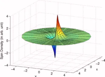
⌫ 共3q˜2+ 2兲 共q˜2+ 2兲共q˜2+ 1兲 − 4q˜2. 共27兲 To restore the conventional units, we addedប into Eqs. 共26兲 and共27兲. The z-component of the spin density in real space is shown in Fig. 2. According to expectations, it has the shape of a dipole oriented perpendicular to the electric field. Its spatial behavior is determined by the single parameter lso, which gives the range of exponential decay of the spin po-larization with increasing distance from an impurity. The Sycomponent averaged over impurity positions gives the uni-form bulk polarization. It is interesting to note that when the target impurities are identical to the background ones 共⌫
⬘
=⌫兲, the so obtained uniform polarization Sy兩q→0 coincidesIII. SPIN ACCUMULATION IN A SEMI-INFINITE SYSTEM
In this section, we will consider a semi-infinite electron gas y⬎0 bounded at y=0 by a boundary parallel to the elec-tric field. Our goal is to calculate a combined effect of spin clouds from random impurities. It is important to note that the summation of spin dipoles from many scatterers does not result in a magnetic potential gradient in the bulk of the sample. This is principally different from the Landauer charge dipoles, which are associated with the macroscopic electric field. The origin of such a distinction can be imme-diately seen from Eq.共26兲. The magnetic potential, as it was defined in Sec. I, is proportional to Sz. By taking its gradient,
one gets qySz. After averaging over impurity positions q →0, qySz→0. It happens due to spin relaxation, which
pro-vides at q = 0 a finite value of the denominator in Eq.共26兲. At the same time, in the case of the charge cloud, the denomi-nator of the particle diffusion propagator is proportional to
q2. Hence, the corresponding gradient of the electrochemical potential 共electric field兲 is finite at q=0. Although the bulk magnetic potential is zero, one cannot expect that it will also be zero near an interface. In order to calculate the spin po-larization near the boundary, Eq. 共21兲, with q=−iⵜ and 2⌫␦共r兲¯␦
ijin the right-hand side, has to be solved using
ap-propriate boundary conditions. With the so obtained Dij共r兲,
the resultant spin density induced by impurities placed at points riis given by Eq.共11兲,
Sj共r兲 =
兺
n=x,y,z冕
d2r
⬘
Djn共r − r⬘
兲Itotn 共r
⬘
兲, 共28兲where the source term is obtained by the inverse Fourier transform of Eq.共19兲: Itot y 共r兲 = v dNfm*␣hk2F 1 ⌫2n i
兺
i ␦共r − ri兲, Itot z 共r兲 = − v dNFhk2F 1 2⌫2n i兺
i y␦共r − ri兲, Itot x 共r兲 = 0. 共29兲where the relation⌫
⬘
=⌫/niis used because we assumed thatthe target impurities are identical to the random ones. The macroscopic polarization is obtained by averaging of Eqs. 共28兲 and 共29兲 over impurity positions. After averaging over xi
and the semi-infinite region yi⬎0, the spin-polarization
source共29兲 transforms to Iavn共y兲:
Iavy共y兲 = vdNFm*␣hkF * 1 ⌫2, Iavz 共y兲 = − vdNFhk2F␦共y − 0+兲 1 2⌫2. 共30兲
It follows from Eq. 共28兲 that the corresponding mean value of the spin polarization, Sav共y兲, satisfies the diffusion equation共21兲 with the source 2⌫Iavn共y兲 in its right-hand side. The so obtained diffusion equation, however, is not com-plete. One should take into account that the boundary itself can create the interface spin polarization. Most easily, it can be done in the framework of the Boltzmann approach. In terms of the Boltzmann function, the spin density is defined as Sav共y兲=兺kgk, and the charge density as兺kgk. The
equa-tion for the Boltzmann funcequa-tion can be written in the form 共see, e.g., Ref.26兲
vgⵜygk+ 2共gk⫻ hk兲 + eEx gk共0兲
kx
=1
关SE共y兲 − gk兴, 共31兲
where SE共y兲=␦共E−EF兲Sav共y兲/NF and gk
共0兲= −h
k␦共E−EF兲 is
the equilibrium Boltzmann function. The terms proportional to the charge component of the Boltzmann function have been omitted in Eq.共31兲 due to the system local electroneu-trality, at least in the scale of the mean free path, which is the smallest characteristic scale of gkspatial variations. The
scat-tering part of Eq.共31兲 is written in the simple relaxation time approximation. Such a scattering term follows26 from the
Keldysh formalism assuming isotropic scattering from impu-rities, as has been adopted in this work. For angular depen-dent scattering, however, a structure of the scattering term is more complicated.27
The spin-polarization source associated with the boundary is given by a direct action of the electric field, without taking into account secondary scattering from impurities. Hence, the term with Sav共y兲 in the right-hand side of Eq. 共31兲 can be ignored. Also, the boundary independent bulk part of gkhas
to be subtracted from the general solution of Eq.共31兲. The so obtained interface Boltzmann function will be denoted as
gkif. The corresponding spin density is Sif共y兲=兺kgkif. In
or-der to calculate gkif, Eq.共31兲 has to be supplemented with the
boundary condition. For a hard wall specularly reflecting boundary, the condition is simply
FIG. 2. 共Color online兲 Spatial distribution of Szcomponent of the spin density around a single scatterer. The unit of length =lso.
兩gkx,ky兩z=0=兩gkx,−ky兩z=0. 共32兲
This condition means that the spin orientation does not change after specular reflection from the interface. The solu-tion of Eq.共31兲 satisfying Eq. 共32兲 can be easily found. As a result, up to o共␣2兲, we obtain
Sify共y兲 = Sifx共y兲 = 0, Sifz共y兲 = 8vd␣2m*
兺
ky⬎0
ky␦共Ek− EF兲e−y共m
*/k
y兲. 共33兲
Within the diffusion approximation, the second of these equations represents a delta source of the spin polarization with intensity 1
冕
0 ⬁ dySifz共y兲 = vdNFhkF 2 1 ⌫. 共34兲This source is exactly of the same magnitude, but opposite in sign to the spin polarization emerging from impurities, which is represented by the integral of 2⌫Iavz 共y兲, with Iavz 共y兲 given by Eq.共30兲. Taking into account that both sources are located at the interface, so that they cancel each other out, one sees that only the y-component of the source originating from impurity scattering retains in the diffusion equation which acquires the form
2S av z y2 − 4m *␣Sav y y − 8m *2␣2S av z = 0, 2S av y y2 + 4m *␣Sav z y − 4m *2␣2S av y = −2⌫ DIav y . 共35兲
The bulk solutions of this equation are Savz = 0 and Savy ⬅Sb
= 2eENF␣, which coincide with the polarization obtained
from Eqs.共26兲 and 共27兲 at q→0.
In order to calculate the spin polarization near the inter-face, we employ the hard wall boundary conditions6,8,9 for
Eq. 共35兲. Such boundary conditions can be easily obtained from Eq.共31兲 by performing its summation over k and inte-grating from y = 0 to some point y0, placed at a distance much larger than l but still small compared to lso. A simple analysis of Eq.共31兲 shows that up to o共␣2兲, the sum over k of the vector product in the left-hand side of Eq.共31兲 can be neglected, while the right-hand side and the term containing the electric field turn to zero identically. As a result, we get
1 m*
兺
k ky兩gkx,ky兩y=y0= 1 m*兺
k ky兩gkx,ky兩y=0. 共36兲According to Eq.共32兲, the above sum is zero at y=0. Hence, it is also zero at y = y0. The latter sum coincides with the spin current within its conventional definition,26 where a
contri-bution associated with the charge density due to the second term of the velocity operator共3兲 is ignored in an electroneu-tral system. Using the gradient expansion of Eq. 共31兲, this current can easily be expressed26 through S
av
j 兩y=0, its y
de-rivative, and the last term in the left-hand side of Eq.共31兲. In this way, one arrives at the boundary conditions from Refs. 6, 8, and 9. We generalize these conditions by adding
pos-sible effects of the surface spin relaxation共see also Ref.10兲. These additional terms are characterized by the two phenom-enological parametersyandz. Finally, we obtain
− D
冏
Sav z共y兲 y冏
y=0+ 2Dm *␣关S av y共0兲 − S b兴 = −zSav z 共0兲, − D冏
Sav y共y兲 y冏
y=0 − 2Dm*␣Savz 共0兲 = −ySav y共0兲. 共37兲One can easily see from Eqs.共35兲 and 共37兲 that atx/y= 0, the
homogeneous bulk solutions Savz = 0 and Savy = Sbturn out to be
the solutions of the diffusion equation everywhere at y⬎0. Therefore, in this particular, case, the z-components of spin clouds from many impurities completely cancel each other out and there is no spin accumulation near the interface. This result, as well as boundary conditions共37兲 for the hard wall case, agrees with Refs.6–9. A different result has been ob-tained, however, in Ref.10, where a method similar to Ref.8 has been employed. Such a distinction requires a special analysis outside the goals of the present work.
Wheni⫽0, the out-of-plane component of the spin
den-sity is not zero. In the case of weak surface relaxation, i
ⰆD/lso, one obtains the following from Eqs.共37兲 and 共35兲:
Savz 共0兲 = 0.35yeE
1
2បD, 共38兲
where we insertedប to restore conventional units. It is inter-esting to note that in such a regime of small enoughi, the
surface polarization does not depend on the spin-orbit con-stant.
IV. SPIN-HALL RESISTANCE AND ENERGY DISSIPATION As it was defined in the Introduction, the interface spin-Hall resistance is given by
RsH=
Savz 共0兲 NFj
, 共39兲
where j is the dc density, j =E, with the Drude conductivity = ne2/ m*. The so defined spin-Hall resistance is closely related to the additional energy dissipation which takes place due to spin accumulation and relaxation near the interfaces of a sample. Indeed, as was shown in Ref.6, the spin accu-mulation is associated with a correction to the electric con-ductivity of the dc flowing in the x-direction. For the Rashba SOI, the correction to the current density has the form
⌬j共y兲 = − e 4m* ␣2k f 2 ⌫2 Savz y . 共40兲
This expression is finite within the distance of⬃lsofrom the interface. After integration over y, one obtains a correction to the electric current,
⌬I = e 4m* ␣2k F 2 ⌫2 Sav z 共0兲. 共41兲
The corresponding interface energy dissipation 共per unit of the interface length兲 can be expressed from Eqs. 共39兲 and 共41兲 as
⌬W = ⌬IE = m*
eប3␣
2R
sHj2. 共42兲 In its turn, RsHcan be determined from Eq. 共38兲. It can be easily seen that⌬W⬎0 ify⬎0.
V. RESULTS AND DISCUSSION
Summarizing the above results within the drift diffusion theory, we found out that the intrinsic spHall effect in-duces in 2DEG a nonequilibrium spin density around a spin-independent isotropic elastic scatterer. The z-component of this density has the shape of a dipole directed perpendicular to the external electric field, while the polarization parallel to 2DEG is isotropic. Due to the D’yakonov-Perel’ spin relax-ation, the spin density decays exponentially at a distance larger than the spin-orbit precession length. It is noteworthy that such a cloud exists even in the case of the Rashba spin-orbit interaction when the macroscopic spin current is absent. We also calculated the macroscopic spin density near an in-terface by taking the sum of clouds due to many scatterers and independently averaging over their positions. Surpris-ingly, in the case of the hard wall boundary, the so calculated spin polarization exactly coincides with that found from the drift diffusion or Boltzmann equations.6–9 In this case, the
out-of-plane component of the spin polarization is zero, while the parallel polarization is a constant determined by the electric spin orientation.15 Besides the hard wall bound-ary, we also considered a more general boundary condition containing the interface spin relaxation, or the spin leaking term. For such a general case, Sz⫽0. This polarization can
be associated with the local magnetic potential because the system attains its local equilibrium within the Sz spatial variation scale, which is much larger than l. The magnetic potential, in its turn, is related to the dc electric current den-sity via the interface spin-Hall resistance. The latter was shown to determine the additional energy dissipation due to the relaxation of the spin polarization near the interface.
Besides conventional semiconductor quantum wells, the results of this work can be applied to metal adsorbate sys-tems with strong Rashba-type spin splitting in the surface states.28 In this case, the spin cloud can be measured by a scanning-tunneling microscope with a magnetic tip.
ACKNOWLEDGMENTS
This work was supported by RFBR Grant No. 060216699, NSC 95-2112-M-009-004, the MOE-ATU Grant, and NCTS Taiwan. We are grateful to the Centre for Advanced Study in Oslo for their hospitality.
1H.-A. Engel, E. I. Rashba, and B. I. Halperin, cond-mat/0603306
共unpublished兲.
2S. Murakami, N. Nagaosa, and S.-C. Zhang, Science 301, 1348
共2003兲; J. Sinova, D. Culcer, Q. Niu, N. A. Sinitsyn, T. Jung-wirth, and A. H. MacDonald, Phys. Rev. Lett. 92, 126603 共2004兲; D. Culcer, J. Sinova, N. A. Sinitsyn, T. Jungwirth, A. H. MacDonald, and Q. Niu, ibid. 93, 046602共2004兲.
3M. I. Dyakonov and V. I. Perel, Phys. Lett. 35A, 459共1971兲; J. E.
Hirsch, Phys. Rev. Lett. 83, 1834共1999兲.
4Y. K. Kato, R. C. Myers, A. C. Gossard, and D. D. Awschalom,
Science 306, 1910共2004兲.
5J. Wunderlich, B. Kaestner, J. Sinova, and T. Jungwirth, Phys.
Rev. Lett. 94, 047204共2005兲.
6A. G. Mal’shukov, L. Y. Wang, C. S. Chu, and K. A. Chao, Phys.
Rev. Lett. 95, 146601共2005兲.
7R. Raimondi, C. Gorini, P. Schwab, and M. Dzierzawa, Phys.
Rev. B 74, 035340共2006兲.
8O. Bleibaum, Phys. Rev. B 74, 113309共2006兲.
9Y. Tserkovnyak, B. I. Halperin, A. A. Kovalev, and A. Brataas,
cond-mat/0610190共unpublished兲.
10V. M. Galitski, A. A. Burkov, and S. D. Sarma, Phys. Rev. B 74,
115331共2006兲.
11İ. Adagideli and G. E. W. Bauer, Phys. Rev. Lett. 95, 256602
共2005兲.
12B. K. Nikolić, S. Souma, L. P. Zârbo, and J. Sinova, Phys. Rev.
Lett. 95, 046601共2005兲; Q. Wang, L. Sheng, and C. S. Ting, cond-mat/0505576共unpublished兲.
13R. Landauer, IBM J. Res. Dev. 1, 223共1957兲; Philos. Mag. 21,
863共1970兲.
14A. G. Mal’shukov and C. S. Chu, Phys. Rev. Lett. 97, 076601
共2006兲.
15V. M. Edelstein, Solid State Commun. 73, 233共1990兲; J. I. Inoue,
G. E. W. Bauer, and L. W. Molenkamp, Phys. Rev. B 67, 033104共2003兲.
16R. S. Sorbello and C. S. Chu, IBM J. Res. Dev. 32, 58共1988兲; C.
S. Chu and R. S. Sorbello, Phys. Rev. B 38, 7260共1988兲.
17W. Zwerger, L. Bönig, and K. Schonhammer, Phys. Rev. B 43,
6434共1991兲.
18A. A. Abrikosov, L. P. Gor’kov, and I. E. Dzyaloshinskii, Meth-ods of Quantum Field Theory in Statistical Physics共Dover, New
York, 1975兲.
19B. L. Altshuler and A. G. Aronov, in Electron-Electron Interac-tions in Disordered Systems, edited by A. L. Efros and M. Pollak
共North-Holland, Amsterdam, 1985兲.
20M. I. D’yakonov and V. I. Perel’, Sov. Phys. JETP 33, 1053
共1971兲 关Zh. Eksp. Teor. Fiz. 60, 1954 共1971兲兴.
21A. G. Mal’shukov and K. A. Chao, Phys. Rev. B 71, 121308共R兲
共2005兲.
22J. I. Inoue, G. E. W. Bauer, and L. W. Molenkamp, Phys. Rev. B
70, 041303共R兲 共2004兲.
23E. G. Mishchenko, A. V. Shytov, and B. I. Halperin, Phys. Rev.
Lett. 93, 226602共2004兲.
24A. A. Burkov, A. S. Nunez, and A. H. MacDonald, Phys. Rev. B
70, 155308共2004兲.
25A. G. Mal’shukov and K. A. Chao, Phys. Rev. B 61, R2413
共2000兲.
26C. S. Tang, A. G. Mal’shukov, and K. A. Chao, Phys. Rev. B 71,
195314共2005兲.
27A. V. Shytov, E. G. Mishchenko, H.-A. Engel, and B. I. Halperin,
Phys. Rev. B 73, 075316 共2006兲; N. A. Sinitsyn, A. H. Mac-Donald, T. Jungwirth, V. K. Dugaev, and J. Sinova, cond-mat/ 0608682共unpublished兲.
28C. R. Ast, D. Pacile, M. Falub, L. Moreschini, M. Papagno, G.
Wittich, P. Wahl, R. Vogelgesang, M. Grioni, and K. Kern, cond-mat/0509509共unpublished兲.