路側雷達偵測器之自動化學習演算法研發

國

立

交

通

大

學

運輸科技與管理學系

博

士

論

文

路側雷達偵測器之自動化學習演算法研發

The Study of Automated Learning Algorithms

for Road-Side Radar Traffic Detector

研 究 生：陳昱光

指導教授：卓訓榮 教授

周幼珍 副教授

Traffic information is essential to effectively perform numerous traffic operations, including travel time estimation or prediction, congestion control policies, and traffic signal control strategies. Traditionally, gathering traffic information is extremely labor and cost intensive, meaning the assistance of advanced information technology equipment is crucial. For overcoming the defects of traditional detectors, the road-side radar detector is adopted in this study, and more advanced learning algorithms are developed to achieve the automation and enhance the accuracy.

The basic traffic information includes traffic count, vehicle classification and ve-hicle speed estimation. Counting traffic in a single lane is a basic task that can be achieved by using traffic detectors to detect passing vehicles, but it is difficult for road-side radar detectors to simultaneously detect different vehicle types in multi-lane environments, because the signals reflected from passing vehicles in a single lane influ-ence neighboring lanes. The spread of reflected signals created difficulty in accurately identifying lanes. Hence, this study first develops a learning procedure for road-side radar detectors to form an on-line traffic lane estimator. An on-line traffic lane es-timator is modelled by Gaussian mixture model (GMM) based on span and conflict information and trained by using the proposed variant of expectation maximization (EM) algorithm. The numerical results demonstrate on-line traffic lane estimator can work well in real-world scenarios, and the accuracy of traffic lane estimator is verified by counting traffic in different lanes.

Besides, the real-time vehicle classifier for road-side radar detectors in multi-lane environments is for the first time presented. A two-dimensional Gaussian Mixed

ii

Model is employed to develop the learning model based on FMCW radar data. An EM algorithm is thus implemented to maximize the likelihood of the formulated learning model; consequently, the model could be used for classifying small and large vehicles in multi-lane environments simultaneously, so that traffic information can be obtained at a relatively lower cost. In the suburban field test, the accuracy of real-time vehicle classifier in multi-lane environments can achieve more than 88%.

I would like to thank Dr. Hsun-Jung Cho and Yow-Jen Jou, my supervisors, for their many suggestions and constant support during this research. I am also thankful to committee members and Dr. Da-Yin Liao for his guidance through the early years of chaos and confusion.

I should also mention that my graduate studies in Taiwan, R.O.C. were supported by MOE ATU Program of the Ministry of Education, Taiwan, R.O.C. and the Na-tional Science Council.

Of course, I am grateful to my parents for their patience and love. Without them this work would never have come into existence (literally). In addition, my aunties also do me a great of help in my study life.

Finally, I wish to thank the following: Pei-Jen Yeh (for her generousness and

love); Dr. Shu-Cherng Fang and Dr. Yi-ming Li (for their knowledge of optimization), Dr Chia-Tung Lee (for his philosophy in life), Dr. Gau-Rong Liang (for his globalized economic view), Dr. Shie-Yuan Wang (for his knowledge of simulation) and many NCTU faculty (for sharing with their knowledge); Heng Huang, Akin, Banana, Urnus, Amie, Tesseric; (for their help in developing radar detectors); Isoguava, Hogan, ... (for all the good times in basketball court and gym); all the Cho-lab members (for all the good and bad times we had together); and my brother (because he asked me to).

National Chiao Tung University, Hsinchu Yu-Kuang Chen

June, 2009

Table of Contents

1.2 Characteristics of Radar-Based Detectors . . . 4

1.3 Problem Description . . . 6

1.4 Research Scope . . . 10

1.5 Research Framework and Organization . . . 11

2 Literature Review 13 2.1 Literature Review for Lane Boundary Estimation . . . 13

2.2 Literature Review for Radar-Based Vehicle Classification . . . 16

3 Road-Side Radar System Design 19 3.1 Hardware Architecture and Design Specifications . . . 20

3.2 Software Architecture . . . 28

3.2.1 Developing Tools and Environment . . . 28

3.2.2 Requirements of Software Design . . . 29

3.2.3 Software Framework . . . 29

4 Background Adapter 32 4.1 Operational Flow Chart of Background Adapter . . . 33

5 Lane Boundary Estimator 37

5.1 Extraction of Span and Conflict Information . . . 38

5.1.1 Span Information . . . 39

5.1.2 Conflict Information . . . 40

5.2 Incorporating a Variant of EM Algorithm with a GMM . . . 43

5.2.1 Gaussian Mixture Model . . . 43

5.2.2 A Variant of EM Algorithm . . . 44

5.2.3 Learning Procedure . . . 49

6 Vehicle Classifier 52 6.1 Automatic Learning Framework . . . 52

6.1.1 Vehicle Detection Algorithm . . . 53

6.1.2 Vehicle Feature Extraction . . . 56

6.1.3 Two-Dimensional Gaussian Mixed Model . . . 57

6.2 Estimation of Vehicle Speed . . . 59

7 Numerical results 61 7.1 Field Test of Lane Boundary Estimator . . . 61

7.1.1 Results of Single-Value Information . . . 62

7.1.2 Results of Span and Conflict Information . . . 65

7.1.3 Motorcycles and Lane Change . . . 69

7.2 Field Test of Vehicle Classifier . . . 70

8 Conclusion 77

Bibliography 79

List of Figures

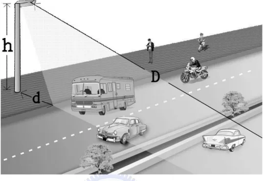
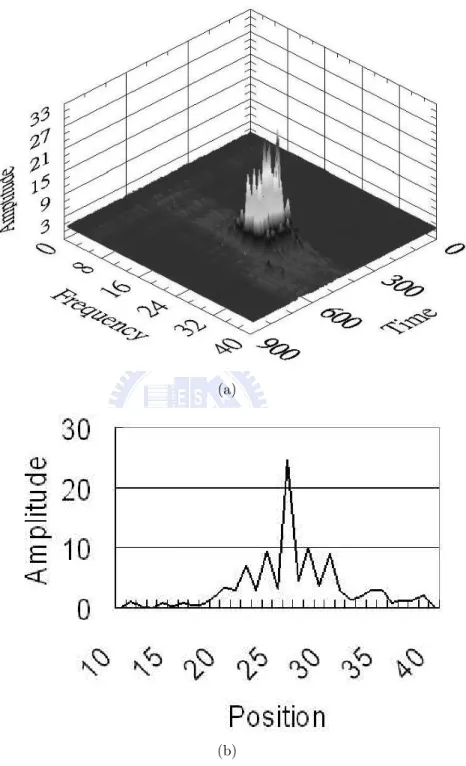
1.1 Sketch map of a multi-lane scenario. The road-side radar detector is mounted at height h, and its illuminative direction is perpendicular to the traffic direction. The least h must be above the height of passed vehicles in the nearest lane for preventing the far reflected signals are entirely blocked by the near vehicles. . . 5 1.2 Frequency-domain information: (a) 3D pattern of a passed vehicle; (b)

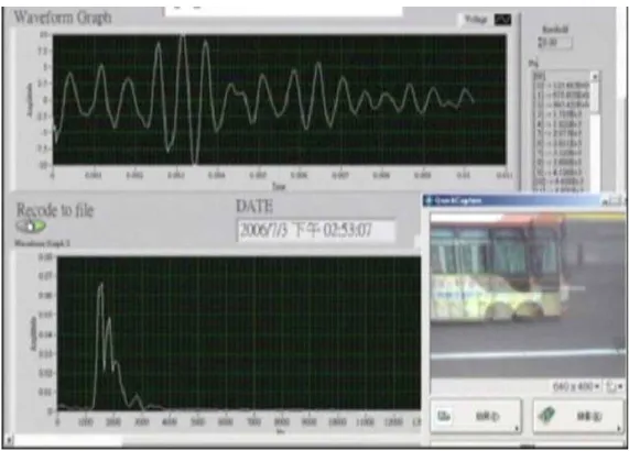
Frequency-domain frame, which is a snapshot of (a), and the scale of x-axis is approximately 78 cm thick. . . 7 1.3 The top figure shows the snapshot of the received voltage signals when

the bus shown in the image was within the illuminative field of the road-side radar, and the bottom figure shows the frequency-domain

frame that is obtained by converting received voltage signals via FFT. 8

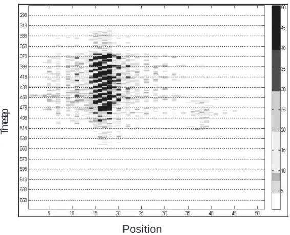
1.4 Energy comparisons between large and small vehicles. This panel data represent that these exists a large vehicle in lane 2 and a small vehicle in lane 6. . . 9 1.5 The organization of this study . . . 12

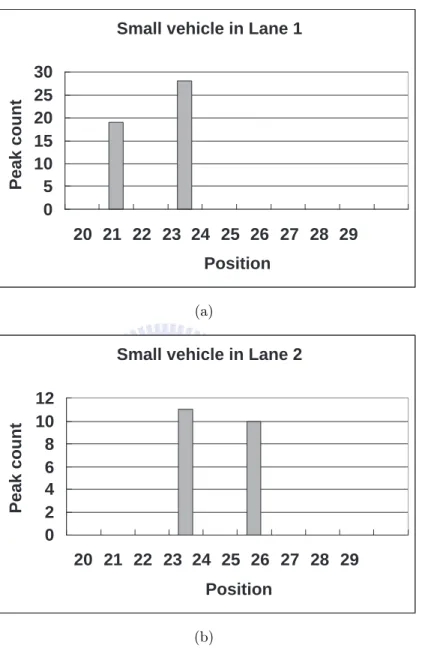
2.1 Examples illustrating the accumulated peak count scenario arose from two vehicles passed through the detection zones in two lanes. (a) indi-cates the accumulated peak count when a small vehicle passed through the detection zone in lane 1, it reveals that position 23 has the maxi-mum bin count. (b) indicates the scenario where a small vehicle passes through the detection zone in lane 2, but position 23 still has the

max-imum bin count. . . 15

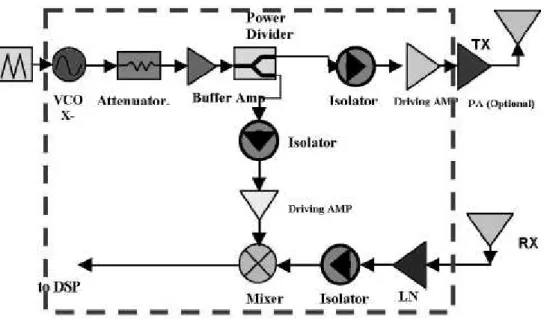
3.1 Block diagram of the X-band FMCW radar system which is composed of two antenna arrays, a single-chip CMOS transceiver (enclosed by the dashed line) and an external digital signal processing unit. Power amplifier is added to increase the output power level [16] . . . 21

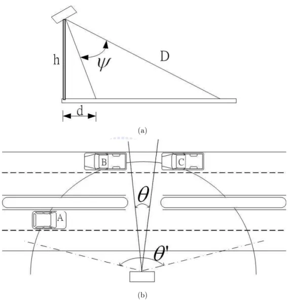
3.2 (a) A side view of road-side radar detector in multi-lane circumstances. (b) A top view of road-side radar detector in multi-lane circumstances. There are a small angle θ and a large angle θ0. . . 25

3.3 E-Plane (Microstrip Leaky-EH1-Mode Antenna Array) [16] . . . 26

3.4 H-Plane (Microstrip Leaky-EH1-Mode Antenna Array) [16] . . . 27

3.5 The C code is deployed on a DSP device, while the java code is deployed on a PC. The devices are connected by RS232, and communicated by the designed interface. . . 28

3.6 The software framework . . . 31

4.1 Flow chart of a background adapter . . . 35

5.1 Learning procedure of the on-line traffic lane estimator . . . 50

5.2 Illustrative example of the learning procedure . . . 51

6.1 Automatic learning framework of real-time vehicle classifier. The first step is to retrieve the real-time voltage data, and the voltage date are large enough to generate 200 frequency-domain frames per second uniformly. . . 53

viii

6.2 Virtual vehicle detection. (a) is a scenario that a virtual vehicle exists,

and (b)(c) show there may be two vehicles in the adjacent lanes. . . . 55

7.1 Real-world experimental environments in the suburbs. (a) is a sunny scenario, and (b) is a rainy scenario. . . 62 7.2 The histogram is the accumulated vehicle count mentioned in the

patent [11]. That is; a single passing vehicle contributes just one count to the corresponding bin. . . 63 7.3 The learned Gaussian distribution density functions of GMM based on

the histogram shown in Figure 7.2, (a)(b)(c)(d) are the results obtained by an EM algorithm associated with different initials. . . 64 7.4 The histograms of real-world data. The top histogram is for the

accu-mulated span information, while the lower histogram is for the conflict information. . . 66 7.5 (a) is the learned Gaussian distribution density functions obtained by

using an EM algorithm, and (b) is the outcome obtained by using the variant of EM algorithm. The difference in learning results between (a) and (b) is that the variance of Gaussian components in (b) is not bigger than that in (a) underlying the same span and conflict information. Both of results are more accurate than that shown in Figure 7.3, and which indicated that the span and conflict information are superior to single-value information . . . 67 7.6 A motorcycle scenario and its histogram of peak count. This case

shows that the track of motorcycle is not proper to describe the lane boundary information. . . 70 7.7 A lane change scenario of a small vehicle and its histogram of peak

count. It indicates that the lane-changing behavior of vehicle is also

not proper to describe the lane boundary information. . . 71

7.8 (a) shows the scatter diagram in lane 2. (b) shows the scatter diagram in lane 3. . . 72

7.9 The learned result of a two-dimensional GMM for lane 2. . . 75

List of Tables

2.1 Literature review for vehicle classification based on radar-based systems 17

3.1 Comparison of the current commercial products . . . 24

7.1 Summary of vehicle types in a multi-lane environment, which includes motorcycles, small vehicles (i.e., Honda civic, Toyota Camry, Volks wagan T4), and large vehicles (i.e., cement, gravel truck, and large bus). . . 63

7.2 The learned parameters of GMM are obtained by an EM algorithm . 65

7.3 The learned parameters of GMM are obtained by the variant of EM algorithm . . . 65 7.4 The classifying results (including vehicles exhibit lane-changing

behav-ior). . . 69 7.5 The classifying results only consider small and large vehicles, and the

passed vehicles do not exhibit lanechanging behavior when passing through the detection area. . . 69 7.6 Lane range . . . 70 7.7 GMM parameters for lane 2. The component with the smaller mean

represents the small vehicles, and the component with the larger mean represents the large vehicles. . . 73

7.8 Compare learned results and real-world date for lane 2. The diagonal counts are vehicles that are classified correctly, and non-diagonal counts are erroneous results. . . 73 7.9 GMM parameters for lane 3. The component with the smaller mean

represents the small vehicles, and the component with the larger mean represents the large vehicles. . . 74 7.10 Compare learned results and real-world date for lane 3. The diagonal

counts are vehicles that are classified correctly, and non-diagonal counts are erroneous results. . . 74

Chapter 1

Introduction

1.1

Motivation

Traffic information is essential to effectively perform numerous traffic operations, in-cluding travel time estimation or prediction, congestion control policies, and traffic signal control strategies. Traditionally, gathering traffic information is extremely labor and cost intensive, meaning that the assistance of advanced information tech-nology equipment is crucial. As IT develops, numbers of detectors have increased. All of this IT equipment has been developed to replace traditional detectors owning to its inexpensiveness, installation flexibility.

Generally speaking, traffic count technologies can be classified into two categories: the intrusive and non-intrusive methods. The former consist of a data recorder and a sensor placing on or in the road. These detectors have been employed for many years and are briefly introduced as follows [1][2][3][4]:

• Pneumatic road tubes: rubber tubes are placed on road lanes to detect passed

vehicles from pressure changes. The pulse of air is detected and recorded by a

traffic counter. The main drawback is that its efficiency is subject to tempera-ture, and low speed flows.

• Piezoelectric sensors: the principle is to convert the mechanical energy to

elec-trical signal. The amplitude of the signal is proportional to the degree of defor-mation.

• Magnetic loops: it is the most common technology applied to collect traffic

data. The loops are embedded in roadways in a square formation that generates a magnetic field. This has a generally short life expectancy because it is usually damaged by heavy vehicles, but is not affected by weather conditions. The main drawback are the implementation and maintenance costs can be expensive. Not-intrusive detectors are remote observations. Even if manual counting is the most common way, some new technologies have recently emerged and should be noted.

• Manual counts: it is the most labor-intensive way. The trained observers collect

traffic flows, pedestrians and vehicle types by using tally sheet, mechanical count boards to record.

• Passive and active infra-red: the presence, speed and type of vehicles are

de-tected and recorded based on infrared equipments. The main drawbacks include bad weather, and limited lane coverage.

• Passive magnetic: it is also embedded in roadways, and it can count the number

of vehicles, type, and speed.

• Ultrasonic and passive acoustic: these detectors transmit sound waves to detect

3

over the lane, and the passive acoustic sensors are placed alongside the road, respectively. The main drawback of both detectors is that the performance is affected by temperature and bad weather (e.g. low temperatures, snow).

• Microwave radar: it can detect moving vehicles, speed and type, and the main

advantage is the performance is not affected by weather conditions, lights.

• Video image detection: video cameras record vehicle numbers, type and speed

by different image processing technologies (e.g. detecting and tracking). The main drawback is that video detectors are very sensitive to light and weather conditions.

Different detectors have different advantages and limitations. In sum, ultrasonic or acoustic sensors in noisy environments are not suitable for use. For inductive loop or magnetic sensors, the installment usually spoils the road pavement and tends to be damaged by passed vehicles. Video and laser sensors are deeply affected by the different conditions of weather and lights. Though these sensors already have high accuracy in traffic count and vehicle type classification [5][6][7], most of sensors (except for video ones) are limited to apply to a single lane environment, such that installation and maintenance costs in cities become very high.

Regarding capability of being applied to multi-lane environments, only video-based and radar-video-based detectors have made great progress. Notably, the video-video-based and radar-based detectors are capable of providing traffic counts, real-time vehicle speed, and vehicle classification simultaneously in multi-lane environments. In other words, detectors are not designed for a specific function. The development of video-based detectors are earlier than radar ones, because video equipments are easier to

be acquired, and image processing techniques are much mature. For video-based de-tectors, except for the effects arose from lights and weather, several environmental variations will affect the accuracy of vehicle analysis. First, vehicle shadows degrade the accuracy of video-based detectors, and lead to erroneous traffic counts. Second, the camera perspective makes vehicles geometry features inconsistent, hence, a cali-bration process is required in advance to fit in with video algorithms [8][9].

1.2

Characteristics of Radar-Based Detectors

Actually, the characteristics of radar-based detectors are better than that of video-based ones. For examples, radar detectors are not influenced by weather effects (such as, heavy fog, rain) and light effects (such as, shadow, dark); hence radar-based detectors eliminate the need for complex algorithms for handling these scenarios in video-based ones. Additionally, radar-based detectors do not need rigorous fine adjustments in setup, and the installation process does not spoil the road pavement. Owing to its high adaptability and inexpensiveness (in multi-lane environments), radar detectors become one of the popular equipments used in traffic surveillance system gradually.

The installation methods of radar-based detectors are classified into two major categories, including looking and side-fire (or road-side) ways. The forward-looking detectors have the illuminative direction parallel to the direction of traffic, and such an installation method is only applied to a single lane. On the other hand, the side-fire approach means that the illuminative direction of radar detectors is per-pendicular to the traffic direction shown in Figure 1.1. The main differences in func-tion between video-based and radar-based detectors include (i) the forward-looking

5

Figure 1.1: Sketch map of a multi-lane scenario. The road-side radar detector is mounted at height h, and its illuminative direction is perpendicular to the traffic direction. The least h must be above the height of passed vehicles in the nearest lane for preventing the far reflected signals are entirely blocked by the near vehicles. approach is the most common installation method for video-based detectors to ap-ply to multi-lane environments. (ii) Video-based detectors usually adopt background subtraction techniques to sense vehicles from a video sequence without knowing the locations of traffic lanes in advance [8][10].

Figure 1.1 is a sketch of a multi-lane environment, and indicates that the road-side radar detector is mounted at height h and at distance d from the nearest lane, while the maximal distance for detecting passing vehicles is D. A road-side traffic detector transmits and receives electromagnetic signal across its illuminative field. The relative distance and the corresponding magnitude information among targets and a detector can be obtained by using a Fast Fourier Transform (FFT) to convert

the received time-domain voltage values into the frequency-domain information. Figure 1.2(a) shows a 3D frequency-domain information of a passed vehicle, and Figure 1.2(b) shows a frequency-domain frame which is a snapshot of Figure 1.2(a). The magnitude of each FFT bin shows the amount of energy of the received signal at a particular frequency, and which depends on the geometry, angles, relative distances and material characteristics of a target vehicle. The frequency shown in Figure 1.2(a) represents the relative distance; hence the vehicle’s position can be directly estimated from the frequency-domain information. For convenience, all figures mentioned later will use position rather than frequency to represent the relative distance. The panel data shown in Figure 1.4 represent a large vehicle in lane 2 and a small vehicle in lane 6, and depict the energy distributions of large and small vehicles. Figure 1.4 also shows that the spread of reflected signals of a large vehicle is so large that neighbor lanes are influenced.

1.3

Problem Description

Road-side radar-based systems have so much advantageous features; nevertheless, road-side radar-based systems do not have very reliable and robust algorithms in the vehicle detection application. Restate, road-side radar-based systems still en-counter various different difficulties in attaining the following functions, including traffic count, vehicle type classification, and speed estimation in multi-lane situations, owing to the spread of the reflected signals resulting from limitations in bandwidth and equipment. It is known that the accurate lane boundary positions are required in multi-lane situations because the boundary positions are fundamental information to carry out all those functions such as a vehicle classifier and speed estimator. Since

7

(a)

(b)

Figure 1.2: Frequency-domain information: (a) 3D pattern of a passed vehicle; (b) Frequency-domain frame, which is a snapshot of (a), and the scale of x-axis is ap-proximately 78 cm thick.

Figure 1.3: The top figure shows the snapshot of the received voltage signals when the bus shown in the image was within the illuminative field of the road-side radar, and the bottom figure shows the frequency-domain frame that is obtained by converting received voltage signals via FFT.

9

Tim

e s

tep

Position

Figure 1.4: Energy comparisons between large and small vehicles. This panel data represent that these exists a large vehicle in lane 2 and a small vehicle in lane 6.

current products do not have robust algorithms to depict the lane boundary positions in various multi-lane situations, such that follow-up functions, such as vehicle type classification, and speed estimation, do not have good performances.

Additionally, the problem of the classification of vehicles arises in many areas such as truck volume estimating, traffic planning, roadway tolling, etc. Thus, how to design a vehicle classifier for distinguishing a large-sized vehicle from a small-sized vehicle in multi-lane situations is very important in software design for road-side radar-based systems.

1.4

Research Scope

The algorithms are proposed for the road-side radar detector to enhance the accuracy of basic functions in multi-lane situations, and meet the following goals.

1. Detect signal variations caused from the environment and update the back-ground information properly.

2. Analyze the defects of the current lane boundary estimation algorithm, and re-design a much accurate one.

3. Analyze and retrieve the characteristics of the passed vehicles, and design a real-time vehicle classifier based on the selected features.

The first problem usually results from intruding objects and the stability of equip-ment. If we have statistical model of the scene, an external intruding object usually spot the parts of signals that don’t fit the model, such as a parked vehicle. Another reason for background variation is the equipment itself, since generated signals would

11

be deeply affected by working temperature and the stability of power supply. Con-sequently, for minimizing these uncertainties, a background adapter is proposed, and this process is usually known as “background subtraction”.

The second problem is how to design a real-time and highly accurate traffic counter in multi-lane situations. For counting vehicles in each lane, the road-side radar should realize where the lane position is, consequently, the development of a lane boundary estimator is required. It is well known that numbers of equipments are designed for a single-lane traffic count, because such a design carried out in a much easier way. However, the quality of current equipments which are able to provide a multi-lane traffic count function still has a great room to improve, because the signals reflected from passing vehicles in a lane influence neighboring lanes.

Lastly, vehicle classification is a very important function for road planning, traffic signal control, and road surveillance applications, because these applications provide useful information for intelligent transportation systems (ITS) to enhance the effi-ciency of traffic operations. Hence, a real-time vehicle classifier is one of the necessary functions to be carried out.

1.5

Research Framework and Organization

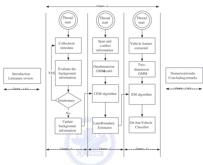
The research framework and organization are shown in Figure 1.5, which describes the required functions of a road-side radar system. Chapter 2 will introduce the related reviews and Chapter 3 introduces an overall system architecture including hardware and software design. After that, three main algorithms will be revealed in Chapter 4, 5, 6, respectively. The aim of Chapter 4 is to develop a background adapter to accommodate environmental changes, such as an intruding parked car or

Thread start Collect real-time data Evaluate the background information Is stationary YES Span and conflict information One dimension GMM model CEM algorithm Two-dimension GMM Vehicle feature extracted EM algorithm Lane Boundary Estimator On-line Vehicle Classifier

Chapter 4 Chapter 5 Chapter 6

Update background information Introduction Literature review Chapter 1 & 2 Numerical results Concluding remarks Chapter 7 & 8 Chapter 3 No Thread start Thread start

Figure 1.5: The organization of this study

temperature variation. The goal of Chapter 5 is to propose two novel features, span and conflict information, to work with one-dimensional Gaussian Mixed Model, and a classification EM algorithm is also introduced to develop a lane boundary estimator. A two-dimensional Gaussian Mixed Model is proposed in Chapter 6 and employed to develop the learning model based on FMCW radar data, and the model could be used for classifying small and large vehicles in multi-lane environments simultaneously. Finally, Chapter 7 and 8 summarize numerical results in the field test and concluding remarks, respectively.

Chapter 2

Literature Review

In this section, the related literature reviews are introduced. The first part is to review the design of lane boundary estimator for multi-lane environment. However, there is few literatures associated with this topic, since this function may not have widespread applications in real-world. So far there are only two patents that are claimed by the current marketing road-side radar manufacturers.

The second part is to review the design of radar-based vehicle classifiers no matter forward or road-side installations. In addition, the feature selected for classifying vehicles are also reviewed and discussed in detail.

2.1

Literature Review for Lane Boundary

Estima-tion

Essentially, developing an on-line automatic traffic lane estimator can be considered as a clustering problem, as is demonstrated in the patent [11]. This patent uses the same frequency-domain information mentioned above to decide the lane position. After obtaining the similar frequency-domain domain information shown in Figure

1.2, the patent utilizes the peak information to form the vehicle feature. The bin with the maximal amount of energy is termed the peak, and the bin with most peak count is used to represent the corresponding vehicle position. In other words, a single passing vehicle contributes just one vehicle count to the corresponding bin. When the sufficient vehicle data are gathered, Gaussian mixture model (GMM) is introduced to model the probability density of lane position. The peaks of probability function describe the lane center, while the low density parts of GMM distribution represent lane boundaries. The description of lane boundary of radar is just to verify that the passed vehicle belonged to which lane, in fact, the description of lane position may not correspond to the real-world lane position.

However, representing a vehicle position by adding just one vehicle count to a bin may involve bias risk, and such an expression may easily result in misleading and incorrect lane outcomes. The examples shown in Figure 2.1 are selected from real-world data, where Figure 2.1(a) and (b) show the peak counts when small vehicles passed through the detection zone in lanes 1 and 2, respectively. According to the vehicle feature proposed in the patent [11], both Figure 2.1(a) and (b) added one vehicle unit to bin position 23, respectively. In other words, even if Figure 2.1(a) and (b) had different bin spectrums arising from the different vehicles in the different lanes, both cases provided the same feature expression that possibly caused ambiguity in separating the two lanes. The detailed outcomes of the patent [11] will also be exhibited in the latter section.

The patent [12] adopts another approach to describe the lane position based on a set of lane center variables, and utilizes displacement information to adjust the lane center. Restated, every reflected signal when a vehicle passed through the detectable

15

Small vehicle in Lane 1

0 5 10 15 20 25 30 20 21 22 23 24 25 26 27 28 29 Position Peak count (a)

Small vehicle in Lane 2

0 2 4 6 8 10 12 20 21 22 23 24 25 26 27 28 29 Position Peak count (b)

Figure 2.1: Examples illustrating the accumulated peak count scenario arose from two vehicles passed through the detection zones in two lanes. (a) indicates the accu-mulated peak count when a small vehicle passed through the detection zone in lane 1, it reveals that position 23 has the maximum bin count. (b) indicates the scenario where a small vehicle passes through the detection zone in lane 2, but position 23 still has the maximum bin count.

area could comprise zone center information. If the newly formed information is sufficiently close to the existing zones, the nearest zone is updated; otherwise, a new zone is defined based on this new formed information. However, the patent [12] easily result in misleading and incorrect lane number outcomes because of the fixed lane width, consequently, follow-up human interventions are usually required. Although this patent has the advantage of not requiring lane number input in advance, it has the weakness that incorrect estimates of lane number make it necessary to spend a long time adding/removing corresponding lanes and adjusting lane positions.

Both of the above patents transformed reflected signals arising from a passing ve-hicle into single-value information (such as bin position, lane center), as may commit bias in estimating the lane position. The main difference between the two patents is that the former is a batch algorithm, while the latter is a real-time algorithm.

This study focuses on designing an online traffic lane estimator for a road-side radar detector in multi-lane environments. New features (such as span information and conflict information) are introduced to describe lane positions such that the am-biguity in feature expression can be eliminated. Additionally, the variant of EM algorithm is proposed to achieve classification and reduce the variance of each Gaus-sian component.

2.2

Literature Review for Radar-Based Vehicle

Clas-sification

Roe et al. (1992) [13] used FMCW radar (10.525GHz) to classify vehicle types, including bicycle, car, light goods, medium goods, heavy goods, and buses based on

17

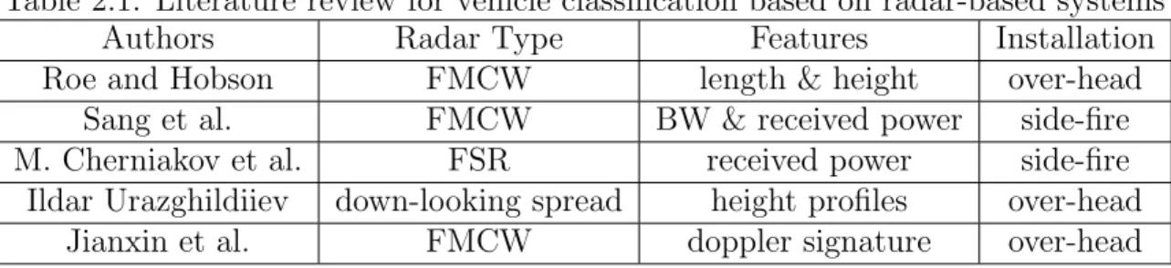
Table 2.1: Literature review for vehicle classification based on radar-based systems

Authors Radar Type Features Installation

Roe and Hobson FMCW length & height over-head

Sang et al. FMCW BW & received power side-fire

M. Cherniakov et al. FSR received power side-fire

Ildar Urazghildiiev down-looking spread height profiles over-head

Jianxin et al. FMCW doppler signature over-head

length and height of cars, and accuracies of 75% in single lane are achieved. Park et al. (2003) [14] developed a K-band (around 24GHz) side-fire FMCW radar for a single lane application, and vehicles are classified as large, medium or small size based on received power and spectrum pattern. Cherniakov (2005) [6] use forward scattering radars (FSR) for classifying ground vehicles, but the transitive and receiving radar antennas are located at different sides of road. Principle component analysis is utilized to reduce dimensionality in frequency-domain feature vector, and the K-nearest is employed to form a classifier. The experimental cars are distinguished into three vehicle categories, including small, medium, and large. The experimental results show that recognition accuracy is only 71% when using the main lobe, while it keeps at 86% without the main lobe. Urazghildiiev et al. (2007) [5] classified vehicles based on vehicle height and length in a single lane, and this exhibits that the signals have the rough geometric pattern similar to the side view of vehicle. The key point of this study is to develop a real-time vehicle classifier for “road-side” equipments in “multi-lane environments”. (1) The road-side equipment is perpendicular to the traffic direction, which makes Doppler effect unapparent to be utilized. (2) The road-side equipment receives the signals of all lanes which requires more sophisticated model and algorithm to describe and analyze our data.

real-world multi-lane applications, there are few significant results and field tests in vehicle classification based on road-side radar detectors. Moreover, using road-side radar detectors for classifying small and large vehicles in multi-lane environments simultaneously will lower the cost of acquiring the traffic information, consequently, this study develops mathematical modelling as a working tool based on FMCW radar data to analyze the vehicle types in multi-lane environments.

Chapter 3

Road-Side Radar System Design

Real-time systems comprises all devices with different constraints and limitations. In general, we can classify these constraints into two categories, that is,“Hard deadlines” and “Soft deadlines”. Hard deadlines are constraints that absolutely must be met. A missed deadline constitutes an erroneous computation and a system failure. In these systems, late data are bad data. On the contrary, if late data are still good data, such a system is referred to a “soft” real-time system. In this study, when the term real-time is used alone, we specifically referring to hard real-time systems [15].

In addition, this study only focuses on the details of software design, thus the hardware design is out of our research scope. However, our proposed softwares are working on the certain requirements of hardware, so these requirements of hardware design will also be briefly introduced in the following section.

3.1

Hardware Architecture and Design

Specifica-tions

An X-band CMOS-based frequency-modulation continuous-wave (FMCW) radar sys-tem is proposed by Tzuang et al. [16] and adopts two antennas to transmit and receive signal separately. The radio frequency (RF) transceiver is formed by standard 0.18

µm one-poly six-metal (1P6M) complementary metal-oxide semiconductor (CMOS)

technology and is embedded in a chip area of 1.68 mm × 1.6 mm. The several sig-nificant properties of the FMCW radar are described as follows. First, the linearity of VCO is 3 % while the output frequency is ranged from 10.3 GHz to 10.8 GHz. Second, the on-chip isolation between the transmitting and receiving paths is 55.0 dB at 10.5 GHz, additionally; two planar leaky-mode antenna arrays with a gain of 18 dB are designed. Experiments indicate the isolation between two antenna arrays with a spacing of 5.0 mm is higher than 42.0 dB at 10.5 GHz.

Figure 3.1 illustrates the block diagram of the X-band FMCW radar system, which comprise dual planar antenna arrays at the transmitter output and the receiver input; a 0.18 µm 1P6M CMOS transceiver is responsible for the RF signal processing as shown inside the dashed lines, and a baseband digital signal processing unit is designated for instantaneous and simultaneous assessment of range measurements. Notably, using two antennas rather than only one eliminates the circulator, as is expensive and does not provide sufficient isolation between the transmitter and the receiver.

In the range measurement, the FMCW radar transmits the signals, and receives the reflecting waves from an intruding vehicle. The amplitude of the input triangular

21

Figure 3.1: Block diagram of the X-band FMCW radar system which is composed of two antenna arrays, a single-chip CMOS transceiver (enclosed by the dashed line) and an external digital signal processing unit. Power amplifier is added to increase the output power level [16]

wave directly controls the output frequency of the transceiver. The bandwidth of the modulated signals at the transmitting path, denoted by BW, is equivalent to the frequency difference between the maximum and minimum output frequencies of the voltage controlled oscillator (VCO). Moreover, the modulated-bandwidth over the half-period of the triangular-wave, denoted by Sb, can be calculated by

Sb = BW tm/2

(3.1.1) where tm denotes the period of the triangular wave, and the parameters are set when performing the signal processes. The pulse-repeated-frequency (PRF) is 500.0 Hz; the swept time (Ts) is set to 2.0ms and the period of triangle-wave tm is 0.5 ms.

signals applied to the mixer. If the round trip time for signal propagation between the sensor and the target is less than that of a half-period of a triangular wave, then

Sb can be maintained at a constant value. Suppose the maximum distance R between

the radar and the target is set 60 meter, and the round trip time τ is described as

τ = 2R

c , (3.1.2)

where c represents the speed of light in air. Consequently, the maximum round trip time τ is 0.4µm. The beat frequency fb shown in (3.1.3) also can be obtained if

any reasonable round trip time is given.

fb =

2 × BW

tm

τ. (3.1.3)

On the contrary, the quantity of R also can be calculated by (3.1.4) if fb is given.

R = c × tm× fb

4 × BW . (3.1.4)

The ideal range resolution R0 of the FMCW radar can be estimated as

R0 =

c

2 × BW, (3.1.5)

thus, range resolution R0 is 1.0 meter. Equations (3.1.1) to (3.1.5) illustrate the

principles of FMCW radar for range measurements. These operations are based on the assumption that the frequency modulation is linear. In other words, the slope

of modulation-bandwidth, Sb, must be maintained at a constant value during the

half-period of the input triangular wave. If the output frequency of VCO is not lin-early proportional to the amplitude of input triangular wave, then the linear transfer

23

resolution of the FMCW radar is degraded. Moreover, the signals at the transmitting and receiving paths are assumed to be independent of each other in the FMCW radar. The coupling effects between the transmitting and receiving paths are not included in the above derivations, hence, such leakages could significantly reduce the performance of the FMCW sensor. The design issues, which include linearizing the generating fre-quency modulating signal and eliminating undesired couplings in the radar system, are significant challenges for the proposed single-chip CMOS transceiver.

Figure 3.2 illustrates the illuminative field of the designed antenna [16] from top and side views. The angle ψ shown in Figure 3.2(a) is called elevational plane beamwidth, and is asked to be large, because the larger angle ψ represents that more lanes can be covered. The angle θ shown in Figure 3.2(b) is called horizontal plane beamwidth, and is expected to be small. The design reasons for the horizontal plane beamwidth as θ can be described as follows. First, if the horizontal plane beamwidth displayed as a large angle θ0 shown in Figure 3.2(b), the information about vehicles in which lane can not be caught. Take vehicles A and B for example, vehicles A and B will form the similar frequency-domain information theoretically because both vehicles have the same relative distance to a detector. Therefore, the large horizontal

plane beamwidth θ0 makes different vehicles’ reflected signals overlap in the same

position such that vehicles in which lane can not be recognized. Second, consider-ing the farthest lane (relative to a road-side radar detector), if the horizontal plane beamwidth is θ0, the illuminative field in the farthest lane may contain more than one vehicle, such that road-side radar detectors can not separate vehicles one by one. Take vehicles B and C for example; vehicles B and C will be misled as an only vehicle if the horizontal plane beamwidth is θ0, then the erroneous traffic count occurs in that

Table 3.1: Comparison of the current commercial products

RTMS Smart Sensor The designed

Model 105 product Elevation 45◦ ₈₀◦ ₅₅◦₍₃₅◦ _{∼ 90}◦₎ Azimuth 15◦ ₁₂◦ ₂₀◦ Detection 3 ∼ 60 m 3 ∼ 60 m 3 ∼ 60 m range Range 2m 3m 3m resolution Time 10.0 ms 2.5 ms 2.0 ms accuracy Protocol RS-232 or RS-232 or RS-232 RS-485 RS-485 Power 4.5W 7.5W 5W consumption Temperature −37◦ _{∼ 74}◦_{C −40}◦ _{∼ 75}◦_C Size 16 x 24 x 12 cm 32 x 23 x 7.6 cm 29.3 x 12.2 x 25.5 cm Weight 2.2 kg < 2.27kg 3.5 kg

lane. In a word, the illuminative field of the antenna determines the position of the farthest lane.

Table 3.1 shows the comparison of the current commercial products with the proposed radar sensor in this research. There is still room for improvement to the same grade products. Besides, the quality of materials and the shell over the detector may affect antenna radiation patterns such that the farthest distance is unable to be detectable. Additionally, antenna radiation patterns of dual planar antenna arrays

are shown in Fig. 3.3 and 3.4. The 3dB beam width of the antenna array was 20◦ _in

25

(a)

(b)

Figure 3.2: (a) A side view of road-side radar detector in multi-lane circumstances. (b) A top view of road-side radar detector in multi-lane circumstances. There are a small angle θ and a large angle θ0.

27

Node1 {Environment = DSP, Language = C} Node2 {Environment = PC, Language = JAVA} * * RS232

Figure 3.5: The C code is deployed on a DSP device, while the java code is deployed on a PC. The devices are connected by RS232, and communicated by the designed interface.

3.2

Software Architecture

For simplifying the developing complexity and analyzing the signals, real-time mod-ules, video and signal retrieval interface cards, are equipped and integrated into an industry PC for simultaneously recording real-world signal and video data. The collected data can be replayed and analyzed through some integrated development environment (IDE), and also can be an off-line input of alpha testing.

3.2.1

Developing Tools and Environment

Our real-time developers use GNU plug-ins embedded on eclipse IDE, and then de-velops the operational C codes that are further executed in the target platforms. For enhancing the developing efficiency, the Concurrent Versions System (CVS) is introduced to help us integrate different versions of functions. For example, bugs sometimes creep in when software is modified, and you might not detect the bug until a long time after you make the modification. With CVS , you can easily retrieve old versions to see exactly which change caused the bug.

In addition, analysis tools and graphic interfaces are developed based on Java language (jfreechart-1.0.8), and the Java programs can be executed at any machine

29

with Java virtual machine (JVM). The communication protocol between the target platforms and analysis tools is defined, and is connected by RS-232 physically. The physical and software deployments is shown in Figure 3.5.

3.2.2

Requirements of Software Design

Based on the sampling capability of equipment (200k ∼ 250k) and the designed range resolution (in our experimental design, the bin range is approximately 78 cm thick), there are approximate 400 ∼ 500 FFT frames generated per second. The sampling rate is limited to the chosen equipment, thus the performance of software is the most important key to be noticed. According to the equation (6.1.2) shown in Chapter 6, the minimal active duration can be obtained, and statistic characteristics should be able to represent a passed vehicle. Consequently, how to reduce the cycle time of our designated algorithms is the most part to decide whether the software is workable.

3.2.3

Software Framework

The software framework is shown in Figure 3.6. First, the parameter, the number of lane, is given, because the number of lane is always fixed while the detector was installed, and it is easy for operators to decide by the eyes. After the number of lane is determined, the learning processes are launched.

The first learning process is to form a background adapter which will be detailed in Chapter 4. The main objectives of background adapter are to find out the back-ground information and further detect the backback-ground variation. The backback-ground variation may be arose from a parked vehicle or an accident, hence, any environmen-tal variation should be detected and further filtered out for enhancing the accuracy

of our interesting signals.

The second learning process is to train a lane boundary estimator, the input is reflected FMCW signals and the objective is to determine that reflected signals belong to which lane. The lane boundaries are the necessary conditions for enhancing the accuracy of traffic count and vehicle classification. Consequently, the lane boundary estimator is the core part of road-side radar systems.

In addition, the spread signal should be detected and be further filtered out, because the spread signal influences the proposed vehicle classification algorithm. The spread signal can be treated as some kind of vehicle shadow, and which is proportional to the RCS of detected targets. So far, there is no vehicle classification algorithm designated for the road-side radar detector, because there are too many parameters to be considered and determined in advanced, for example, background information, lane boundaries, and sampling characteristics. In this study, the spread of reflected signals will also be filtered out by integrating certain background information for enhancing the accuracy of vehicle classification, moreover, the boundaries of different vehicle are also be estimated.

Opposite to the current marketing products, the vehicle type will be determined first in our study, the vehicle speed is derived subsequently. Theoretically, the vehicle speed can be estimated directly through the vehicle speed formula of single loop detector if the loop length is given. The estimation of loop length in each lane is out of our research scope, hence, the speed estimation is only proposed theoretically. The functional parts of software are roughly described as above, and the total execution time is asked to be the less the better, because the less execution time means the more sampling of vehicle can be obtained.

31

Input the number of lane Detect and handle background variation

Filter the spread signals of vehicle

Determine vehicle type on each lane Determine vehicles belong to which lane

Estimate the vehicle speed Real-time

radar signal

Background Adapter

The aim of background adapter is to overcome possible changes resulted from cir-cumstances. For example, one of cases is that an intruding car parks in the detection zone after background information retrieved by radar systems. Usually background information is the scenario that the detection zone does not contain any moving ob-jects, in other words, vehicles may park within the detection zone, but not in the moving state. The goal of designing a background adapter is to allow the radar sys-tems to adapt different background patterns for capturing the better signals of passed vehicles, and then further enhances the accuracy of road-side radar systems.

Background subtraction is a common technique to remove non-moving objects from a video sequence for obtaining background information. The traditional ap-proach is to select several video sequences containing no moving objects and then take a weighted average of the current background and the current frame of the video sequence [17][18][19][20].

A false alarm is an erroneous radar target detection decision caused by noise exceeding the detection threshold. In general, it is an indication of the presence of a radar target when there is no valid target. False alarms are generated while

33

thermal noise exceeds a pre-set detection threshold, by the presence of spurious signals (either internal to the radar receiver or from sources external to the radar), or by the malfunction of equipment. If the detection threshold is set too high, there will be very few false alarms, on the contrary, if the threshold is set too low, the large number of false alarms will restrain detection of valid targets. Constant false alarm rate (CFAR) detection refers to a common form of adaptive algorithm that vary the detection threshold as a function of the sensed environment [21][22].

After extracting background information, intruding vehicles which suddenly parked within the detection zone are still valid targets (neither noise or spurious information), consequently, the idea of FAR or CFAR is not a suitable definition for describing the scenario that vehicle parked after background information retrieved by radar systems. There are few literature reviews of background extraction applied for radars, but the idea of background extraction can be also borrowed from video field for overcoming the mentioned scenario. The next subsection will introduce the operational flow chart of background adapter and explain in detail.

4.1

Operational Flow Chart of Background Adapter

The input of background adapter is real-time voltage data, and could be converted to frequency-domain information by Fast Fourier Transform. Based on the capability of equipment, the averaged sample rate is 200k ∼ 250k. According to the designed range resolution 0.78 meters, 512 sampling points are required to form a frame of frequency-domain information. A frame of frequency-domain information at time t is denoted as −→Ft. Consequently, there are 400 ∼ 500 frames generated per second.

because algorithms, such as Fast Fourier Transform, background information update, lane boundary estimation, vehicle type classification and speed estimation, occupy certain “short” time to be executed. Consequently, the less computational burden, the more number of frequency-domain frames can be analyzed.

After obtaining a frequency-domain frame−→Ft, a common background subtraction

technique applied for video-based equipments is employed to extract background in-formation. Background subtraction information −→Rt can be derived based on (4.1.1),

and the magnitude of −→Rt is expressed as

° ° °−→Rt ° ° °. − → Rt= − → Ft− − → Ft−1. (4.1.1)

Moreover, such background subtraction information is updated all the time for detecting any moving objects in the detection area. A pre-set threshold level δ is a small value, and is applied to look for any feasible background information. If °

° °−→Rt

° °

° is less than threshold level δ, it implies there is no moving objects within the detection area, so information will be kept and further be analyzed to detect whether background information changes. If

° ° °−→Rt

° °

° is larger than threshold level δ, a variation, that maybe caused by moving objects, occurs certainly in the detection area. δ can be regarded as a sensitivity measure to detect background changes.

The array size for storing background information is N * P, where P is the num-ber of bin position of frequency-domain domain information, and N is the numnum-ber of frame. Usually, the number of N is set to 500, and the significant level α is set to 0.01. The null hypothesis is that the sample mean of background information is equal to the previously decided background information on the corresponding bin position.

35 1 ! t t t F F R

"

#

R

If the null hypothesis is rejected, background information −→B is updated by the

lat-est background information −→Ft, moreover, if the changed background information is

within the certain lane position, the vehicle classifier on that corresponding lane will be asked to train again. If the null hypothesis is not rejected, the array for storing background information keeps to update if

° ° °−→Rt

° °

Chapter 5

Lane Boundary Estimator

The traffic surveillance function, the most basic and fundamental of all ITS functions, is responsible for gathering continuous, real-time information on the state of the trans-portation system and driving environment. The information gathered forms the basis for the different traffic management and control actions that can be taken to optimize performance and also serves as the basis for the information to be disseminated to travellers [23].

Traffic surveillance has relied upon measuring devices, which have traditionally been embedded into the road, for both measuring traffic conditions and providing control to signaling mechanisms that regulate traffic flow. However, many of sensors have been “intrusive” types. Several “no-intrusive” sensor technologies have been developed for traffic monitoring, however, none of these devices can be reconfigured or adapted without the assistance of certified technicians. Such an on-site modification to the sensors may take several hours to several days for a single reconfiguration.

This section develops a learning algorithm of road-side radar sensors to monitor traffic conditions when vehicles pass through a field of view and process the data into an estimation of the position of each of the detected vehicles. The positions

are defined and recorded for use in a probability density function estimation without requiring manual set-up and definition of the traffic lane boundaries. The update process is done by continuously updating the parameters of the GMM [11].

5.1

Extraction of Span and Conflict Information

In supervised learning, category labels or training patterns are provided to estimate the unknown model parameters to reduce errors or costs. In unsupervised learning or clustering, no category labels or human interventions exist to guide error measure re-duction [24]. Besides, if the instances in the learning problems are characterized by the presence of a small percentage of labelled data or side-information only, such learning algorithms are the ones dubbed as semi-supervised learning. The side-information that could be useful in clustering problems is primarily obtained from background knowledge about the domain or instances [25][26].

Constraint information is one of side-information to form constraints to assist in clustering. Basically, the constraints primarily comprise two types, equivalence con-straints (positive concon-straints, must-link concon-straints) and not-equivalent concon-straints (negative constraints, cannot-link constraints). Equivalence constraints specify two un-labelled instances must belong to the same cluster, while not-equivalent con-straints refer to the situation where the two instances come from different sources [27][28][29][30].

39

5.1.1

Span Information

To overcome the defects in the patents mentioned above, this study proposes a new feature, span information, for building a learning feature rather than adopting only a single sample point to describe lane positions when a vehicle passed through. The span information denotes an idea of a signal range of a single lane width formed by the reflected signal from a passing car.

Conceptually, the idea of span information is analogous to instance-level equiva-lence constraint, because the selected bins come from the same source (same vehicle). In other words, The span information modifies the shape based on background knowl-edge to form learning samples. The span information is carried out by applying the concept of a convex hull to establish a closed set, and by grouping the selected bins that belong to a lane into a closed interval. The closed set comprises the bin po-sitions where peaks had occurred, and should pass through the following two steps to form reasonable information. Notably, vehicles that are applied to form the span information don’t include the motorcycles, because it is meaningless for merging two motorcycles detected on adjacent lanes. Therefore, the motorcycles will be filtered out through the vehicle detection algorithm.

1. “Maximum separation” indicates the maximal distance between the adjacent bin positions with peaks of a passed vehicle. The common distance between the adjacent bin positions is same to the illustrated examples shown in Figure 2.1 that the bin range is approximately 78 cm thick, hence, the reasonable inference that there seldom exists an empty subinterval (for example, a subinterval with a width exceeding 1 meter) in which no peak occurs as a vehicle passes by. Consequently, if the distance between any adjacent bin positions with peaks

is less than 1 meter, the two bins should be grouped into a closed interval. The iterative merging procedure will not stop until the distance between any adjacent bin with peaks is larger than 1 meter. On the contrary, if the distance between any adjacent bin with peaks is larger than 1 meter, the reflected signals should be regarded as two different vehicles.

2. “Maximum extent” describes the maximum reach of the span information. Ac-cording to the regular lane width design, the lane width is about 4 ∼ 5 meter. This design aims to catch reflected signals from individual vehicles, while avoid-ing those from pairs of vehicles in adjacent lanes that are detected and gathered simultaneously. Because such information is inappropriate for addressing a sin-gle lane’s positions, hence, the maximum extent is employed to filter out the vehicles in adjacent lanes that are detected simultaneously.

Restated, the span information is formed by using the above two steps, and which accords with the idea of instance-level equivalent constraint that group the select bins belonging to a vehicle into a closed interval. Take Figure 2.1 for example, the span information in (a) ranges from 21 to 23, while that in (b) ranges from 23 to 25. The primary advantage of span information is that the ambiguous results derived from the mentioned patents can be avoided.

5.1.2

Conflict Information

Besides, for developing the more accurate on-line traffic lane estimator, another fea-ture, conflict information, is extracted to work together with span information. Con-flict information is an idea to represent the lane boundary, and can be directly derived

41

from the property of span information without introducing other external informa-tion. Notably, introducing the external intervention is unrealistic and inappropriate when dealing with a general road environment, because the attention devoted to installation and calibration leads to inconvenience and operational costs.

From the collected data, span information obtained from vehicles in different lanes do not overlap except for boundary positions, therefore, the overlap implies a higher possibility of lane boundaries. For obtaining overlapping positions, this study assumes if the left boundary of span information is same to the right boundary of another, a conflict pair is formed at that position. Conceptually, conflict information is an idea analogous to an instance-level not-equivalent constraint, because different span information arose from vehicles in different lanes can be considered as different sources.

To identify the possible conflict positions on the arrival of span information, an intuitive and heuristic matching mechanism is designed to count the conflict pairs at every position and expressed as follows:

Ci = min{L[i], R[i]}, (5.1.1)

where the conflict count at position i, denoted as Ci, and L[i] and R[i], respectively,

denoted the accumulated left and right boundary counts of span information on po-sition i. Taking Figure 2.1 as an example, the span information of a small vehicle in lane 1 is 21-23, thus, the left boundary is 21 and the right boundary is 23 (L[21] = 1 and R[23] = 1). Additionally, the span information of a small vehicle in lane 2 is 23-25, hence, the left boundary is 23 and the right boundary is 25 (L[23] = 1 and

only a conflict pair is derived at position 23, and the conflict count is one; that is

C23= 1.

Furthermore, if the histogram of accumulated span information can take the con-flict information provided by Eqn. (5.1.1) into account, the resultant accumulated his-togram more closely reflects vehicle distribution. Hence, the accumulated hishis-togram of span information is further adjusted by incorporating the conflict information ac-cording to the following Eqn. (5.1.2)

A0_i = min{Ai− Ci}, (5.1.2)

where the accumulated counts on position i denoted as Ai and the refined

accumu-lated counts on position i denoted as A0_i. In sum, conflict information is an outcome generated by the different span information without knowing that span information belongs to which lane, and is generated by the on-line panel data without the guide-lines provided by external experts or teachers, hence, the whole learning process can be executed automatically.

Additionally, even if vehicles rarely pass through one of lanes, the subtraction of the accumulated span information by using conflict information still should be implemented. Since conflict information usually appears at the boundary of span in-formation, and just occupies a small part of span information. Hence, the subtraction of conflict counts will not make that the lane with rare vehicles becomes less apparent. On the contrary, the adjustment for the accumulated span information will sharpen the distribution so that lane positions can be described more precisely.

43

5.2

Incorporating a Variant of EM Algorithm with

a GMM

5.2.1

Gaussian Mixture Model

Gaussian Mixture Model is a very popular technique for model selection [31][32] and clustering [33], and its purpose is to express the probability density function of the chosen features as a weighted sum of several Gaussian distributions. Owing to the flexibility of GMM, it also has been successfully applied to other applications in re-lation to image processes [34][35][36], speech recognition [37][38], and other fields [39][40][41]. Besides, the Gaussian component also can be replaced by another prob-ability density function to apply to different applications [42].

Generally, large variance results from real-world imperfect or noisy data, and leads to the GMM being ineffective in the clustering problem. Lee and Cho [43] attempted to overcome the weakness of large variance by applying the committee approach, which combines several single models to reduce variance. Banfield and Raftery [44] suggested to use a uniform noisy component to handle noise, and it would also reduce the variance of Gaussian components. The component with small variance is extremely important, particularly in relation to boundary determination, because the large variance may easily result in misleading and incorrect lane position outcomes. As a consequence, the variant of EM algorithm [45] is proposed to reduce the variance of Gaussian components and achieve classification, and is detailed in the following subsection.

5.2.2

A Variant of EM Algorithm

This study develops a variant of EM algorithm to achieve classification and reduce

the variance of each Gaussian component; that is, data point xi is assigned to the

component which has the highest likelihood at the start of each iteration, and each component updates its sample mean and variance by only calculating the instances assigned to it rather than using all instances. The proposed variant of EM algorithm will not stop until such time as difference between consecutive iterations is below some specific tolerance level and none of the instances changed its component. In other words, the variant of EM algorithm can be regarded as a classification version of the EM algorithm. The proposed variant of EM algorithm incorporating the above GMM could form an on-line lane estimator. More formally, a GMM p(x|θ) with M components can be described as:

p(x|θ) = M

X

m=1

αmg(x; µm, σm2), (5.2.1)

where α1, ..., αM denote the non-negative weights and add up to one, while µm and σ2

m, respectively, denote the estimate of the mean and variance of the mth Gaussian

distribution g(x; µm, σ2m) (or gm(x)). Data point xi is assumed i.i.d. where i ∈ {1, 2, . . . , n} and represents the relative distance.

All of GMM parameters θ = [α1, α2, . . . , αM, µ1, µ2, . . . , µM, σ12, σ22, . . . , σM2 ] can be

estimated and optimized by using the variant of EM algorithm, and the expectation of log-likelihood is detailed as follows:

45 E − step : (5.2.2) J(θ|θ(k)₎ = E " ln " _n Y i=1 p(xi) #¯_¯ ¯ ¯ ¯θ (k) # = E " _n X i=1 ln p(xi) ¯ ¯ ¯ ¯ ¯θ (k) # (5.2.3) where θ(k) _{is the estimate at iteration k.}

Additionally, let ¯ ¯ ¯Xj(k) ¯ ¯

¯ denote the set size for data point xi being assigned to

component j which has the highest likelihood at iteration k, and can be expressed as follows:

X_j(k): {i : xi is assigned to the component j at iteration k},

where ¯ ¯ ¯X_j(k) ¯ ¯ ¯ 6= 0, and SM j=1 X_j(k)= {1, 2, 3, ...., n}.

For obtaining the optimal θ, we follow the method of Maximum Likelihood. First, Gaussian density function is differentiated with respect to µ and σ.

∇µg(x; µ, σ2) = g(x; µ, σ2₎¡₋ 1 2σ2 ¢ ∇£(x − µ)T_{(x − µ)}¤ = g(x; µ, σ2₎³(x−µ) σ2 ´ ∇σg(x; µ, σ2) = (2π)−d/2    (−d)σ−d−1_exph₋(x−µ)T_(x−µ) 2σ2 i + σ−dh(x−µ)T_(x−µ) σ3 i exp h −(x−µ)_2σT2(x−µ) i    = g(x; µ, σ2₎³(x−µ)T_(x−µ) σ3 −_σd ´

For simplifying the expression, the β_j(k)(xi) = α(k)_j g_j(k)(xi)δ(k)_ij M P j=1α (k) j g (k) j (xi)δij(k) is introduced. The

update rules are obtained by differentiating Eqn. (5.2.3) with respect to µj, and

σj, and the update formula for the parameters for each component are addressed as

follows. ∇µjJ(θ) = n P i=1 αjg(xi;µj,σ2j)δij α1g(xi;µ1,σ21)δi1+α2g(xi;µ2,σ22)δi2+...+αMg(xi;µM,σ2_M)δiM (xi−µj) σ2 j = PN i=1 βj(xi) ³ (xi−µj) σ2 j ´ ∇σjJ(θ) = PN i=1 αjg(xi;µj,σ2j)δij α1g(xi;µ1,σ21)δi1+α2g(xi;µ2,σ22)δi2+...+αMg(xi;µM,σ2_M)δiM ³ (x−µ)T_(x−µ) σ3 j − d σj ´ = PN i=1 βj(xi) ³ (x−µ)T_(x−µ) σ3 j − d σj ´

where δ_ij(k)is a binary indicator. δ_ij(k)= 1, if data point xiis assigned to the component j; otherwise δ_ij(k)= 0; that is δ(k)_ij = 1.

According to the first order necessary condition for optimality, let ∇µjJ(θ) = 0

and ∇σjJ(θ) = 0. Consequently, M − step can be addressed as follows:

α(k+1)_j = P i∈X_j(k) β_j(k)(xi) P j P i∈Xj(k) β_j(k)(xi) (5.2.4) µ(k+1)_j = P i∈Xj(k) β_j(k)(xi)xi P i∈Xj(k) β_j(k)(xi) (5.2.5) σ2(k+1) j = P i∈X_j(k) β_j(k)(xi)(xi− µ(k)j )2 P i∈X_j(k) β_j(k)(xi) (5.2.6)