運動影片內容分析、理解與註釋之研究

國

立

交

通

大

學

資訊科學與工程研究所

博

士

論

文

運動影片內容分析、理解與註釋之研究

Sports Video Content Analysis, Understanding and Annotation

研 究 生：陳華總

指導教授：李素瑛 教授

運動影片內容分析、理解與註釋之研究

Sports Video Content Analysis, Understanding and Annotation

研 究 生：陳華總 Student：Hua-Tsung Chen

指導教授：李素瑛 Advisor：Suh-Yin Lee

國 立 交 通 大 學

資 訊 科 學 與 工 程 研 究 所

博 士 論 文

A Dissertation

Submitted to Institute of Computer Science and Engineering College of Computer Science

National Chiao Tung University in partial Fulfillment of the Requirements

for the Degree of Doctor of Philosophy

in

Computer Science August 2009

Hsinchu, Taiwan, Republic of China

運動影片內容分析、理解與註釋之研究

研究生: 陳華總 指導教授: 李素瑛 教授

國立交通大學資訊工程學系

摘要

隨著教育、娛樂、運動以及其它各式各樣多媒體應用的發展，數位化的影音多媒體 數位內容與日劇增。因此，許多研究致力於多媒體內容的分析與理解並研發實用的系 統，讓使用者可以快速地獲得所要的多媒體資料。運動影片是影音多媒體資料中相當重 要的一環，有著相當可觀的商業利益、多樣的娛樂效果以及龐大的觀眾群，所以有越來 越多的研究著眼於運動影片分析。目前大多數的運動影片分析以場景分類或精彩片段的 擷取為主。然而，有越來越多的觀眾或球員希望能有多媒體系統的輔助來取得更豐富的 運動資訊。甚至，裁判也要求利用電腦技術來輔助判決以提高公平性。本論文研究重點 在於單一視角之視訊特徵的整合並設計相關演算法以達成運動影片內容理解、索引、註 釋與擷取。 在運動影片中，重要的事件主要發生於球跟球員之間的互動。為了得知意義上與戰 術上的相關內容，首先我們提出了一個有效且快速的方法來追蹤球路並計算球在各畫面 中的位置。球路追蹤是一個相當艱難的問題。球在畫面中的體積小且不明顯，移動速度 又快，想在單一畫面中辨別出哪一個物體是球，幾乎是不可能的。因此，我們利用球在 畫面中移動的特性來辨識哪一段軌跡是球路，而不是從各畫面中去辨識哪一個物體是 球。為了取得更豐富的比賽資訊並對比賽內容有更深刻的理解，我們提出一套創新的方 法，能夠從單一視角之影片重建3D 球路。此 3D 球路重建之演算法可用於籃球、排球、

網球之類擁有特定球場模型且多數場地特徵能被鏡頭所拍攝到之運動影片。在這類的運 動影片中，利用攝影機所拍攝到的球場邊線與特徵物體，可以計算出三維空間位置與二 維畫面座標之間的轉換關係。要從二維資訊去推論三維的資訊本來就是相當具有挑戰性 的一個問題，因為在影像拍攝的過程中已經損失了空間中的深度資訊。在此，我們利用 物理特性來設立球在三維空間的移動模型，再加上先前所求計算得之二維軌跡以及三維 二維間的轉換關係，我們將可以估算出三維球路模型的參數，進而重建球在三維空間的 運動軌跡。所取得之二維球路與重建之三維球路在運動影片中有著多樣化的重要應用， 像是籃球的投籃出手點定位、排球事件偵測，以及棒球的投球球路分析。從三維球路所 產生之三百六十度虛擬重播更可以讓觀眾隨己意變換不同視角來觀看球的動向。 在棒球比賽中，投球的進壘點（球經過打者時，與好球帶的相對位置）是影響球被 打擊出去後移動方向的一個重要因素。好球帶是決定投球進壘點的一個參考指標，因此 我們提出了一演算法分析打者姿勢與輪廓來設定好球帶，不論左打或右打姿勢都可適 用。除了投打之間的對決外，球被打擊出去後的守備過程亦是吸引觀眾注目的焦點。經 由辨識畫面中的特徵物體與線段，我們分類目前攝影機所拍攝的球場區域。因為攝影機 所拍攝之區域即為事件發生之區域，所以我們可以利用影片中不同球場區域之轉換來推 論球的移動路線與防守過程，並提供相似防守片段之比較，以分析守備策略。 我們以籃球、排球與棒球影片為測試資料，進行了多樣的實驗來評估所提出各種方 法的效能。在我們的實驗中，其結果驗證所提各方法之可行性與優越性，並顯示從單一 視角之運動影片即可取得相當多的比賽內容資訊供球員、教練做戰術分析與資料統計之 用，並讓觀眾對比賽有更深入的了解。我們亦相信，本論文所提之運動資訊擷與影片內 容理解諸多方法將可以應用於更多種類之運動影片。

Sports Video Content Analysis, Understanding and Annotation

Student: Hua-Tsung Chen Advisor: Prof. Suh-Yin Lee

Department of Computer Science,

National Chiao Tung University

Abstract

The explosive proliferation of multimedia data in education, entertainment, sport and various applications necessitates the development of multimedia application systems and tools. As important multimedia content, sports video has been attracting considerable research efforts due to the commercial benefits, entertainment functionalities and a large audience base. The majority of existing work on sports video analysis focuses on shot classification and highlight extraction. However, more keenly than ever, increasing sports fans and professionals desire computer-assisted sports information retrieval. Even more, the umpires demand assistance in judgment with computer technologies. In this thesis, we concentrate on the feature integration and semantic analysis for sports video content understanding, indexing, annotation and retrieval from single camera video.

In sports games, important events are mainly caused by the ball-player interaction and the ball trajectory contains significant information and semantics. To infer the semantic and tactical content, we first propose an efficient and effective scheme to track the ball and compute the ball positions over frames. Ball tracking is arduous task due to the fast speed and small size. It is almost impossible to distinguish the ball within a single frame. Hence, we utilize the ball motion characteristic over frames to identify the true ball trajectory, instead of recognizing which object is the ball in each frame. To retrieve more information about the

games and have a further insight, we design an innovative approach of 3D ball trajectory reconstruction in single camera video for court sports, where the court lines and feature objects captured in the frames can be used for camera calibration to compute the transformation between the 3D real world and the 2D frame. The problem of 2D-to-3D inference is intrinsically challenging due to the loss of the depth information in picture capturing. Incorporating the 3D-2D transformation and the physical characteristic of ball motion, we are able to approximate the depth information and accomplish the 2D-to-3D trajectory reconstruction. Manifold applications of sports video understanding and sports information retrieval can be achieved on the basis of the obtained 2D trajectory and the reconstructed 3D trajectory, such as shooting location estimation in basketball, event detection in volleyball, pitch analysis in baseball, etc. The 3D virtual replay generated from the 3D trajectory makes game watching a whole new experience that the audience are allowed to switch between different viewpoints for watching the ball motion.

In baseball, the pitch location (the relative location of the ball in/around the strike zone when the ball passes by the batter) is an important factor affecting the motion of the ball hit into the field. Strike zone provides the reference for determining the pitch location. Hence, we design a contour-based strike zone shaping and visualization method. No matter the batter is right- or left-handed, we are able to shape the strike zone adaptively to the batter’s stance. Computer-assisted strike/ball judgment can also be achieved via the shaped strike zone. In addition to the pitcher/batter confrontation, the defense process after the ball is batted also attracts much attention. Therefore, we design algorithms to recognize spatial patterns in frames for classifying the active regions of event occurrence in the field. The ball routing patterns and defense process can be inferred from the transitions of the active regions captured in the video. Furthermore, the sequences with similar ball routing and defense patterns can be retrieved for defense strategy analysis.

conducted to evaluate the performance of the proposed methods. The experimental results show that the proposed methods perform well in retrieving game information and even reconstructing 3D information from single camera video for different kinds of sports. It is our belief that the preliminary work in this thesis will lead to satisfactory solution for sports information retrieval, content understanding, tactics analysis and computer-assisted game study in more kinds of sports videos.

誌 謝

首先，最感謝的是指導教授李素瑛老師。六年的博士班期間，李老師在研究上的諄 諄善誘與耐心教誨，才讓我得以成就此篇博士論文。李老師在生活態度、待人處世，以 及各方面應對進退上給我的教導，都讓我終身受益無窮。此外，在我難過的時候，老師 給了我關心；在我沮喪的時候，老師給了我鼓勵；在我茫然的時候，老師給了我指引。 這一切都讓我銘感於心。 感謝蔡文錦老師在論文研究方面的指導。也感謝蔡老師在生活上對我的幫助與鼓 勵，讓我知道人生還是可以有新的目標。感謝杭學鳴教授在計畫書口試、校內口試以及 校外口試時提供寶貴的建議與鼓勵。感謝所有口試委員：吳家麟教授、廖弘源教授、范 國清教授、張隆紋教授在口試過程中不吝提供多年的珍貴研究經驗，充實了本論文的深 度與廣度，使本論文更趨完善。諸位口試委員都是我在學術研究上最佳學習典範。 感謝學長陳敦裕博士在研究上的熱心指導與心得分享，並在我遭遇困挫時給我鼓勵 與幫助。資訊系統實驗室的學長與學弟妹都是我博士班研究生涯的好夥伴，感謝並祝福 大家早日收穫豐富的研究成果。 感謝交大排球校隊、資工系排、應數女排的成員們，有了你們的陪伴，讓我的博士 生涯中增添了不少歡笑與感動。感謝在我最低潮的時候陪我一起走過的朋友們，因為有 你們的關心、鼓勵與陪伴，才讓我有繼續走下去的勇氣。 家人給予我的關懷與支持讓我在博士求學過程中無後顧之憂。一路走來，父母從不 給我壓力，總是給予我溫暖的關懷。妹妹與弟弟的關心，以及對於父母的照顧，更是讓 我能夠勇往直前的動力。有了他們的辛苦與支持，才有今日的我。感恩家人與其它親友 對我的祝福與勉勵。 要感謝的人很多，在此向所有曾經幫助關心過我的人，致上最真切的謝意。 僅以此論文，獻給關心與幫助過我的大家。

Table of Content

摘要 ………...i

Abstract ………...iii

誌謝 ……….vi

Table of Content ………vii

List of Figures ………..x

List of Tables………..xvi

Chapter 1. Introduction……….………..1

Chapter 2. Physics-based Ball Tracking and 3D Trajectory Reconstruction with Applications to Shooting Location Estimation in Basketball Video ………….6

2.1 Introduction…………..………6

2.2 Overview of the Proposed Physics-Based Ball Tracking and 3D Trajectory Reconstruction System in Basketball Video………...…………9

2.3 Court Shot Retrieval………...………11

2.4 Camera Calibration………...……….13

2.4.1 White line pixel detection……….………...15

2.4.2 Line Extraction……….………...17

2.4.3 Computation of camera calibration parameters………...18

2.5 2D Shooting Trajectory Extraction………19

2.5.1 Ball candidate detection………..………19

2.5.2. Ball tracking……….………..23

2.6 3D Trajectory Reconstruction and Shooting Location Estimation……….…………27

2.7 Experimental Results and Discussions in Basketball Video……….……….29

2.7.1 Parameter setting……….29

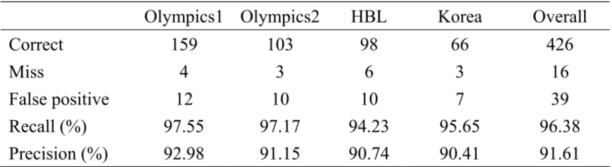
2.7.3 Results of court line and backboard top-border detection………..………….31

2.7.4 Performance of basketball tracking and shooting location estimation………32

2.7.5 Comparison and discussion……….………35

2.8 Summary………...……….37

Chapter 3. Ball Tracking and 3D Trajectory Approximation with Applications to Tactics Analysis in Volleyball Video……….………...39

3.1 Introduction………40

3.2 Related Work……….……….41

3.2.1 Related work on camera calibration……….41

3.2.2 Related work on ball/player tracking……….……….42

3.3 Overview of the Proposed Ball Tracking and 3D Trajectory Approximation in Volleyball Video……….………..44

3.4 Audio Event Detection………...45

3.4.1 Whistle detection……….………46

3.4.2 Attack detection……….………..46

3.5 Camera Calibration………47

3.6 2D Volleyball Trajectory Extraction………..……….48

3.6.1 Ball candidate detection………..………48

3.6.2 Potential trajectory exploration……….………..49

3.6.3. Trajectory identification and integration………51

3.7 3D Volleyball Trajectory Approximation………..……….52

3.8 Trajectory-Based Applications in Volleyball Games……….……….57

3.8.1 Action detection and set type recognition using 2D trajectory……….……..57

3.8.2 3D virtual replays and serve placement estimation using 3D trajectory ……58

3.9 Experimental Results and Discussion in Volleyball Video………….………59

3.9.2 Results of 2D volleyball trajectory extraction……….………60

3.9.3 Simulation results of 3D volleyball trajectory approximation………63

3.9.4 Comparison with Kalman filter-based algorithm………..………..67

3.10 Summary……….……….68

Chapter 4. Sports Information Retrieval in Baseball Video...……….69

4.1 Introduction………70

4.2 Trajectory-Based Baseball Tracking Framework……….………72

4.2.1 Moving object segmentation……….………..73

4.2.2 Ball candidate detection……….……….74

4.2.3 Candidate distribution analysis and potential trajectory exploration………..75

4.2.4 Trajectory identification……….……….76

4.2.5 Baseball trajectory extraction………..77

4.2.6 Trajectory-based pitching evaluation and visual enrichment………..79

4.3 Automatic Strike Zone Determination………..……….82

4.3.1 Overview of the proposed strike zone determination algorithm……….……84

4.3.2 Home plate detection………87

4.3.3 Batter region (BR) outlining……….………..88

4.3.4 Batter contouring……….………....88

4.3.5 Dominant point locating……….……….90

4.4 Baseball Exploration using Spatial Pattern Recognition………93

4.4.1 Visual feature extraction……….……….94

4.4.2 Spatial pattern recognition………..96

4.4.3 Play region type classification………....97

4.5 Experimental Results………100

4.5.1 Results of trajectory-based baseball tracking……….………..101

4.5.3 Results of play region classification…….………110

4.6 Summary………..……….111

Chapter 5. Conclusions and Future Work……….………113

Lists of Figures

Fig. 1-1. Overview of the proposed framework……….2 Fig. 2-1. Statistical graph of shooting locations: O (score) or X (miss)………9 Fig. 2-2. Flowchart of the proposed system for ball tracking and 3D trajectory reconstruction

in basketball video……….11

Fig. 2-3. Examples of shot types in a basketball game: (a) Court shot; (b) Court shot; (c)

Medium shot; (d) Medium shot; (e) Close-up shot; (f) Out-of-court shot…………12

Fig. 2-4. Examples of Golden Section spatial composition: (a) Frame regions; (b) Court view;

(c) Medium view………13

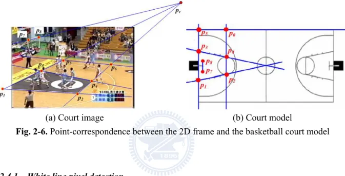
Fig. 2-5. Flowchart of camera calibration………...15 Fig. 2-6. Point-correspondence between the 2D frame and the basketball court model: (a)

Court image; (b) Court model………...15

Fig. 2-7. Illustration of part of an image containing a white line……….16 Fig. 2-8. Sample results of white line pixel detection: (a) Original frame; (b) Without

line-structure constraint; (c) With line-structure constraint………16

Fig. 2-9. Detection of backboard top-border: (a) Detected court lines; (b) Computing vanishing point; (c) Searching backboard top-border………18

Fig. 2-10. Color histograms of 30 manually segmented basketball images………20 Fig. 2-11. Illustration of ball pixel detection: (a) Source frame; (b) Moving pixels; (c)

Extracted ball pixels………...21

Fig. 2-12. Left: detected ball candidates, marked as yellow circles. Right: motion history

image to present the camera motion: (a) Fewer ball candidates produced if the camera motion is small; (b) More ball candidates would be produced if there is large camera motion………...23

Fig. 2-13. Diagram of a long shoot………..25 Fig. 2-14. Relation between Vb an H………...25 Fig. 2-15. Illustration of ball tracking process(X and Y represent ball coordinates)………..26 Fig. 2-16. Illustration of the best-fitting function………27

Fig. 2-17. Statistical data of the shot lengths for different basketball shot classes…………..30

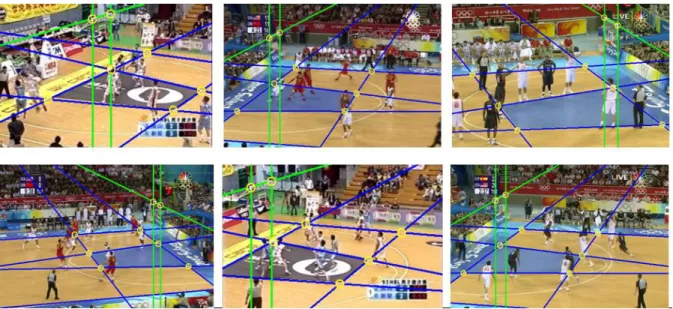
Fig. 2-18. Example results of detecting court lines and corresponding points (marked with yellow circles)………...32

Fig. 2-19. Example of a shooting trajectory being separated………...33

Fig. 2-20. Demonstration of shooting location estimation. In each image, the blue circles are the ball positions over frames, the green circle represents the estimated shooting location and the red squares show the movement of corresponding points due to the camera motion.………...34

Fig. 2-21. Example of directional deviation in 3D trajectory reconstruction: (a) Shooting location estimation; (b) 3D virtual replay……….35

Fig. 2-22. Error case of shooting location estimation caused by the misdetection of backboard top-border: (a) Corresponding points; (b) shooting location estimation…………...35

Fig. 2-23. Comparison of shooting location estimation with/without vertical (height) information: (a) Original shooting location in the frame; (b) Estimated shooting location with vertical information; (c) Estimated shooting location without vertical information.………37

Fig. 3-1. Framework overview of the proposed VIA system………...44

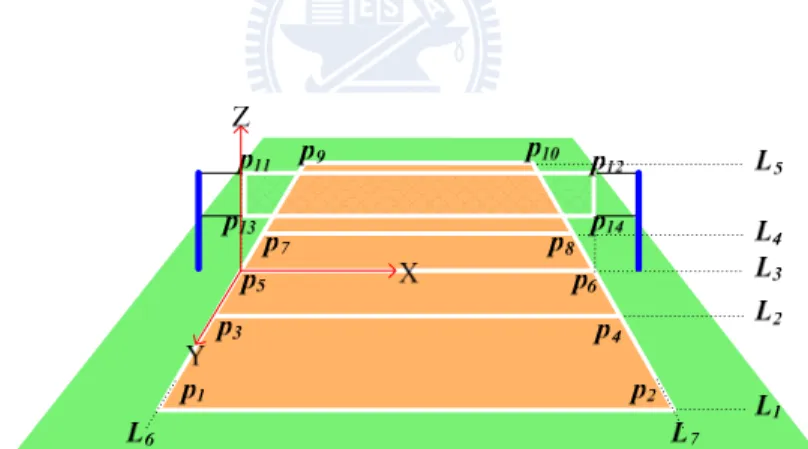
Fig. 3-2. Illustration of the non-coplanar feature points………..47

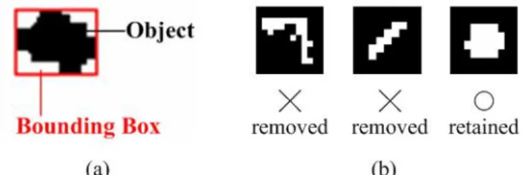
Fig. 3-3. Illustration of the compactness filter: (a) Compactness degree Dcompact is defined as the ratio of the object size to the area of the bounding box; (b) Objects with low Dcompact would be removed while objects with high Dcompact would be retained.…..48

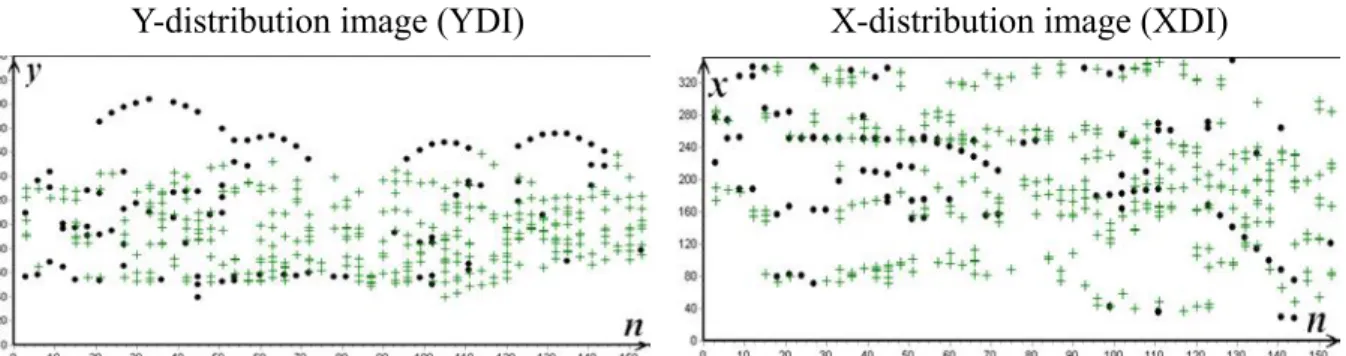
Fig. 3-4. Illustration of the Y- and X-distribution images for different process stages of a volleyball game: (a) Plotting the y-and x- coordinates of the ball candidates over time (indexed by the frame serial number n). Black dots represent isolated candidates and green crosses represent contacted candidates; (b) Potential trajectories: the sequences of the linked ball candidates in YDI and XDI; (c) Integrated trajectory………..50

Fig. 3-5. Procedure of potential trajectory exploration……….51

Fig. 3-6. Procedure of 3D trajectory approximation………55

Fig. 3-7. Illustration of set type diagram………...58 Fig. 3-8. Illustration of volleyball detection and ball tracking: (a) Original frame; (b) Ball

detection; (c) Ball tracking………61

Fig. 3-9. Demonstration of ball trajectory extraction and action detection in volleyball video:

(a) Serve; (b) Reception; (c) Set and (d) Attack.………63

Fig. 3-10. Demonstration of 3D trajectory approximation: (a)~(d) The enriched frames for

serve, reception, set and attack, respectively; (e) Ball trajectory projected on the court model; (f) Serve placement estimation; (g)~(h) 3D virtual replays from different viewpoints.………64

Fig. 3-11. Demonstration of 3D trajectory approximation: (a)~(d) The enriched frames for

serve, reception, set and attack, respectively; (e) Ball trajectory projected on the court model; (f) Serve placement estimation; (g)~(h) 3D virtual replays from different viewpoints.………..64

Fig. 3-12. Error case in 3D trajectory approximation: (a) Detected ball candidates of serve; (b)

The 3D approximated trajectory of serve; (c) Detect ball candidates in the video sequence; (d) The 3D trajectory approximated from the ball candidates in (c)…...66

Fig. 3-13. Error case in 3D trajectory approximation: (a) Ground truth 2D ball positions; (b)

Ball candidates detected; (c) and (d) 3D virtual replays from different viewpoints ………66

Fig. 4-1. Block diagram of the proposed baseball tracking framework………73 Fig. 4-2. Illustration of segmenting the moving objects where the ball is included: (a)

Original frame; (b) FDI; (c) PFDI………74

Fig. 4-3. Illustration of the Y- and X-distribution images for different processing stages of

trajectory extraction, where n is the frame serial number, yc in YDI and xc in XDI are the y- and x-coordinates of each candidate in the original frame, respectively. (a) Ball candidate distribution analysis. Black dots represent isolated candidates and green crosses represent contacted ones. (b) Trajectory exploration. Potential trajectories are shown as the linking of ball candidates. (c) Trajectory identification. The ball trajectory identified is shown as the parabolic curve in YDI and the straight line in XDI……….75

Fig. 4-4. Summarized demonstration of baseball trajectory extraction………78 Fig. 4-5. Demonstration of trajectory-based pitching evaluation and visual enrichment. Left:

the superimposed ball trajectory and pitching evaluation. Right: the final ball location spotlighted with a crosshair. (a) Example of a MLB (Major League Baseball) pitch shot with a left-handed pitcher. (b) Example of a JPB (Japan

Professional Baseball) pitch shot with a right-handed pitcher………81

Fig. 4-6. Illustration of strike zone definition………..82

Fig. 4-7. Applications for strike zone determination: (a) Pitch location image; (b) Count of pitches in each region………...84

Fig. 4-8. Sample results of combining ball trajectory extraction with strike zone………….84

Fig. 4-9. Specifications of the baseball, home plate and batter’s boxes………..85

Fig. 4-10. Block diagram of the proposed strike zone determination system………..85

Fig. 4-11. Layout of home plate, batter’s boxes and batter regions……….86

Fig. 4-12. Procedure of home plate detection: (a) Original frame of a pitch scene; (b) Pixels with high intensity around the frame center; (c) Detected home plate.………87

Fig. 4-13. Example of moving edge extraction (within the OBR): (a) Gray level image In; (b) Edge map En; (c) Luminance difference image |In–In–1|; (d) Difference edge map DEn; (e) Moving edge map MEn………89

Fig. 4-14. Procedure of batter contouring………89

Fig. 4-15. Back and front contours for right- and left-handed batters……….91

Fig. 4-16. Dominant point locating using the points of curvature extremes.……….91

Fig. 4-17. Sample results of dominant point locating………92

Fig. 4-18. Strike zone shaping and visualization: (a) A right-handed batter; (b) A left-handed batter………..93

Fig. 4-19. Overview of the proposed baseball exploration framework………93

Fig. 4-20. Prototypical baseball field: (a) Full view of a real baseball field; (b) Illustration of field objects and lines………...94

Fig. 4-21. Spatial distribution of dominant colors and white pixels: (a) First field frame; (b) Hue histogram; (c) Segmented regions; (d) Extracted white pixels……….95

Fig. 4-22. Detection of field lines and field objects……….97

Fig. 4-23. Twelve typical play region types………..98

Fig. 4-24. Scheme of play region type classification within a field shot………...100 Fig. 4-25. Illustration of ball detection and ball tracking in baseball video: (a) Ball detection.

Two ball positions are missed when passing over the white uniform. (b) Ball

tracking. Positions of missed balls can be recovered………..103

Fig. 4-26. Examples of ball tracking and visual enrichment for various baseball clips: (a) MLB pitch shot; (b) JPB pitch shot; (c) CPBL pitch shot………103

Fig. 4-27. Error cases of home plate detection………107

Fig. 4-28. Illustration of Asz, Agt and Aov………...107

Fig. 4-29. P-R distributions of MLB, JPB and CPBL sequences………..108

Fig. 4-30. Example results of strike zone determination………...109

Fig. 4-31. Examples of the improper strike zone determination: (a) Improper batter contouring due to the dynamic advertising board. (b) Improper batter contouring due to the movement of the plate umpire………110

Lists of Tables

Table 2-1. Performance of basketball shot boundary detection………...31

Table 2-2. Performance of basketball court shot retrieval………...31

Table 2-3. Performance of basketball tracking………33

Table 2-4. Performance of basketball shooting location estimation………33

Table 2-5. Comparison between the proposed physics-based method and the Kalman filer- based method in basketball video………..37

Table 3-1. Discriminants of ten common set types………..58

Table 3-2. Performance of whistle detection………...60

Table 3-3. Performance of attack detection……….60

Table 3-4. Performance of volleyball detection and tracking………..61

Table 3-5. Performance of action detection……….62

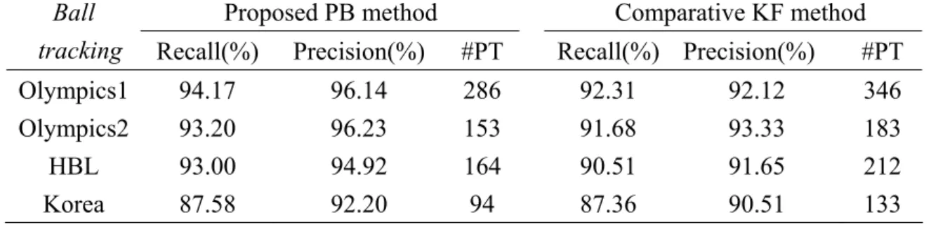
Table 3-6. Comparison between the proposed physics-based method and the Kalman filer- based method in volleyball video………..67

Table 4-1. Ball speed estimation with five-star evaluation using the ball trajectory………...80

Table 4-2. Trajectory curvature measurement with five-star evaluation.………...80

Table 4-3. Rules of play region type classification………..99

Table 4-4. Testing data used in the experiments………100

Table 4-5. Performance of baseball detection and tracking………102

Table 4-6. Comparison between the Kalman filter-based algorithm and the proposed physics-based algorithm in baseball video………105

Table 4-7. Performance of home plate detection………106

Table 4-8. Performance of strike zone determination………108

Chapter 1. Introduction

The advances in video production technology and the consumer demand have led to the ever-increasing volume of multimedia data. The rapid evolution of digital equipments allows general users to archive multimedia data much easily. The explosive proliferation of multimedia data in education, entertainment, sport and various applications makes manual indexing and annotation no more practical. The development of practical systems and tools for multimedia content analysis, understanding, indexing and retrieval is undoubtedly compelling [1, 4, 6, 72, 73, 74].

A large number of content retrieval approaches have been proposed on the basis of low-level features. However, human interpret video in terms of semantics rather than low-level features. The demand for automatic video understanding and interpretation requires the mid-level representations mapping from low-level features to high-level semantics, such as shot class, camera motion pattern, color layout, object shape and object trajectory. Especially, object trajectory is one of the most informative representations which human use to analyze events frequently. Hence, the trajectory-based approaches have been gaining popularity [8, 15, 34, 35].

As important multimedia content, sports video has been attracting considerable research efforts due to the commercial benefits, entertainment functionalities and a large audience base [1, 2, 22, 25, 30, 35, 74]. In this thesis, we take sports video as source material for research. Techniques of event detection, content understanding and sports information retrieval are proposed for automatic annotation and enriched visual presentation. Most viewers prefer retrieving the designated events, scenes and payers to watching a whole game in a sequential way. Therefore, various algorithms have been developed for shot classification, highlight extraction and semantic annotation based on the fusion of audiovisual features and the game-specific rules.

In this thesis, we focus on feature integration and algorithm development for sports video content analysis and understanding. Sports information retrieval, tactics analysis, enriched visual presentation can provide the audience and professionals a further insight into the games. Fig. 1-1 depicts the overview of our research work. We first extract low-level features adaptive to different event detection so as to infer the high-level semantic information. Then, various mid-level representations are computed to bridge the gap between low-level features and semantic content meanings. Since significant events are mainly caused by the interaction of moving objects, object trajectories bring much semantic information contributive to content understanding. Thus, we design several trajectory-based algorithms for sports video content analysis and understanding.

For semantic and tactical content analysis in sports video, we first propose an effective and efficient ball tracking algorithm. Object tracking is usually the medium to convert the low-level features into high-level events in video processing. Object tracking has been an arduous problem despite the long research history. Ball tracking is even a more challenging task due to the fast speed and small size. It is almost impossible to distinguish the ball within a single frame, so information over successive frames, e.g. motion information, is required to facilitate the discrimination of the ball from other objects. In several kinds of ball games, the ball moves following the physical characteristic that the ball trajectory forms a (near-) parabolic curve. For example, the ball shot toward the basket in a basketball game, the ball passed between players in a volleyball game, the ball moving between players in a tennis game and the pitched ball in a baseball game. Utilizing the physical characteristics of ball motion, we present a physics-based ball tracking method to compute the 2D ball trajectory in different kinds of single camera sports videos.

To have a further insight into the games and retrieve more detailed sports information, we propose an innovative approach capable of reconstructing 3D ball trajectory from single camera video for court sports. The 2D-to-3D inference is intrinsically challenging due to the loss of 3D information in projection to 2D frames. For court sports, the court lines and feature objects are captured in video frames. We utilize the domain knowledge of the court specifications to compute the transformation between 3D real world positions and 2D frame coordinates for camera calibration. Involving the physical characteristic of ball motion, we are able to recover the 3D information and reconstruct the 3D ball trajectory.

The obtained 2D trajectory and the reconstructed 3D trajectory enable manifold applications to sports information retrieval and computer-assisted game study. In basketball games, shooting location (the location of a player shooting the ball) is one of the important game statistics providing abundant information about the shooting tendency of a team. The statistical graph of shooting locations facilitates the coach to view the distribution of shooting

locations at a glance and to quickly comprehend where the players have higher possibility of shooting. Then, the players and the couch can infer the offense tactics of an opponent team and adapt their own defense strategy toward the team. Presently, most of the shooting location logging tasks are achieved manually. It is time-consuming and inefficient to watch a whole long video, take records and gather statistics. Thus, we propose a scheme to extract the shooting trajectory in basketball video, reconstruct the 3D trajectory and estimate the shooting location.

In volleyball games, players are not allowed to hold the ball. Hence, we detect the ball-player interaction events by utilizing the positions and the occurring times of direction changes in the trajectory. Moreover, the reconstructed 3D trajectory can provide the sports information the audience or professionals would like to know, such as set type, attack height, serve speed, serve placement, etc. Most of the informative game statistical data which cannot be directly perceived through human eyes can now be obtained based on the obtained 2D trajectory and the reconstructed 3D trajectory. Furthermore, the 3D virtual replay gives an exciting and practical visualization which enables watching the ball motion from any viewpoint.

In baseball games, the ball speed and the curvature of the ball trajectory are two main factors in determining how difficult the pitched ball can be hit. Hence, we track the pitched ball and extract the ball trajectory. Thus, ball speed and trajectory curvature can be computed for pitch analysis. Due to the capturing viewpoint and the frame rate constraint, the ball speed and trajectory curvature might not be very precise. The proposed pitch analysis is not for grading, but for entertainment effects, enriched visual presentation and sports information retrieval. In addition to ball speed and trajectory curvature, the pitch location (the relative location of the ball in/around the strike zone when the ball passes by the batter) also dominates the direction of the ball batted out. For example, a batter who swings at a lower pitch has a good chance of hitting a ground ball, while a batter who swings at a higher pitch

has a great chance of hitting the ball in the air. Since the strike zone provides reference for determining the pitch location, we propose a contour-based method to shape the strike zone according to the batter’s stance. Strike/ball judgment can also be visualized on the video frames by the shaped strike zone. Besides the pitch/batter confrontation, the ball motion and the defense process after the ball is batted into the field is another focus of attention. With the field specifications, we design algorithms to recognize the spatial patterns (field lines and field objects) in frames. Then, the active regions of event occurrence in the field are classified by the spatial patterns. We can infer the ball routing patterns and defense process from the transitions of the active regions captured in the video. Content understanding and annotation can thus be achieved, providing rich information about the games.

Comprehensive experiments on basketball, volleyball and baseball videos show encouraging results. The proposed methods perform well in 2D ball tracking and 3D trajectory reconstruction from single camera video for different kinds of sports. It is our belief that the coach and players will be greatly assisted in game study with the semantic and tactical information derived from our proposed methods. Also, the audience can have a professional insight into the game.

In the following chapters, we give detailed explanation for the proposed methods and techniques. The rest of the thesis is organized as follows. Chapter 2 explains physics-based ball tracking and 3D trajectory reconstruction with applications to shooting location estimation in basketball video. Chapter 3 describes ball tracking and 3D trajectory approximation with applications to tactics analysis in volleyball video. Chapter 4 elaborates on ball tracking, strike zone shaping and play region classification in baseball video. Finally, Chapter 5 concludes this thesis.

Chapter 2. Physics-Based Ball Tracking and 3D Trajectory Reconstruction

with Applications to Shooting Location Estimation in Basketball Video

The demand for computer-assisted game study in sports is growing dramatically. This chapter presents a practical video analysis system to facilitate semantic content understanding. A physics-based algorithm is designed for ball tracking and 3D trajectory reconstruction in basketball video and shooting location statistics can be obtained. The 2D-to-3D inference is intrinsically a challenging problem due to the loss of 3D information in projection to 2D frames. One significant contribution of the proposed system lies in the integrated scheme incorporating domain knowledge and physical characteristics of ball motion into object tracking to overcome the problem of 2D-to-3D inference. With the 2D trajectory extracted and the camera parameters calibrated, physical characteristics of ball motion are involved to reconstruct the 3D trajectories and estimate the shooting locations. Our experiments on broadcast basketball video show promising results. We believe the proposed system will greatly assist intelligence collection and statistics analysis in basketball games.

The rest of this chapter is organized as follows. Section 2.1 gives the introduction. Section 2.2 elaborates the overview of the proposed system. Sections 2.3, 2.4 and 2.5 present the processes of court shot retrieval, camera calibration and 2D shooting trajectory extraction, respectively. Section 2.6 explains on 3D trajectory mapping and shooting location estimation. Experimental results and discussions are presented in section 2.7. Finally, section 2.8 summaries this chapter.

2.1 Introduction

The advances in video production technology and the consumer demand have led to the ever-increasing volume of multimedia information. The rapid evolution of digital equipments

allows the general users to archive multimedia data much easily. The urgent requirements for multimedia applications therefore motivate the researches in various aspects of video analysis. Sports videos, as important multimedia contents, have been extensively studied, and sports video analysis is receiving more and more attention due to the potential commercial benefits and entertaining functionalities. Major research issues of sports video analysis include: shot classification, highlight extraction and object tracking.

In a sports game, the positions of cameras are usually fixed and the rules of presenting the game progress are similar in different channels. Exploiting these properties, many shot classification methods are proposed. Duan et al. [1] employ a supervised learning scheme to perform a top-down shot classification based on mid-level representations, including motion vector field model, color tracking model and shot pace model. Lu and Tan [2] propose a recursive peer-group filtering scheme to identify prototypical shots for each dominant scene (e.g., wide angle-views of the court and close-up views of the players), and examine time coverage of these prototypical shots to decide the number of dominant scenes for each sports video. Mochizuki et al. [3] provide a baseball indexing method based on patternizing baseball scenes using a set of rectangles with image features and the motion vector.

Due to broadcast requirement, highlight extraction attempts to abstract a long game into a compact summary to provide the audience a quick browsing of the game. Assfalg et al. [4] present a system for automatic annotation of highlights in soccer video. Domain knowledge is encoded into a set of finite state machines, each of which models a specific highlight. The visual cues used for highlight detection are ball motion, playfield zone, players’ positions and colors of uniforms. Gong et al. [5] classify baseball highlights by integrating image, audio and speech cues based on maximum entropy model (MEM) and hidden Markov model (HMM). Cheng and Hsu [6] fuse visual motion information with audio features, including zero crossing rate, pitch period and Mel-frequency cepstral coefficients (MFCC), to extract baseball highlight based on hidden Markov model (HMM). Xie et al. [7] utilize dominant color ratio

and motion intensity to model the structure of soccer video based on the syntax and content characteristics of soccer video.

Object tracking is widely used in sports analysis. Since significant events are mainly caused by ball-player and player-player interactions, balls and players are tracked most frequently. Yu et al. [8] present a trajectory-based algorithm for ball detection and tracking in soccer video. The ball size is first proportionally estimated from salient objects (goalmouth and ellipse) to detect ball candidates. The true trajectory is extracted from potential trajectories generated from ball candidates by a verification procedure based on Kalman filter. The ball trajectory computed is applied to analyze semantic basic and complex events, team ball possession and the play-break structure. Some works of 3D trajectory reconstruction are built based on multiple cameras located on specific positions [11-14]. In addition, computer-assisted umpiring and tactics inference are burgeoning research issues of sports video analysis [11-15]. However, these can be considered as advanced applications based on ball and player tracking. Therefore, object tracking is an essential and vital issue in sports video analysis.

In this chapter, we work on the challenging issues of ball tracking and 3D trajectory reconstruction in broadcast basketball video in order to automatically gather the game statistics of shooting locations – the location where a player shoots the ball. Shooting location is one of the important game statistics providing abundant information about the shooting tendency of a basketball team. An example of statistical graph for shooting locations is given in Fig. 2-1, where each shooting location is marked as an O (score) or X (miss). The statistical graph for shooting locations not only provides the audience a novel insight into the game but also assists the coach in guiding the defense strategy. With the statistical graph for shooting locations, the coach is able to view the distribution of shooting locations at a glance and to quickly comprehend where the players have higher possibility of scoring by shooting. Thus, the coach can enhance the defense strategy of the team by preventing the opponents from

shooting at the locations they stand a good chance of scoring. Increasing basketball websites, such as NBA official website, provide text- and image-based web-casting, including game log, match report, shooting location and other game statistics. However, these tasks are achieved by manual efforts. It is time-consuming and inefficient to watch a whole long video, take records and gather statistics. Hence, we propose a physics-based ball tracking system for 3D trajectory reconstruction so that automatic shooting location estimation and statistics gathering can be achieved. Whether the shooting scores or not can be derived from the change of the scoreboard by close caption detection technique [16]. Thus, the statistical graph of shooting locations, as Fig. 2-1, can be generated automatically.

Fig. 2-1. Statistical graph of shooting locations: O (score) or X (miss).

2.2 Overview of the Proposed Physics-Based Ball Tracking and 3D Trajectory Reconstruction System in Basketball Video

Object tracking is usually the medium to convert the low-level features into high-level events in video processing. In spite of the long research history, it is still an arduous problem. Especially, ball tracking is a more challenging task due to the small size and fast speed. It is almost impossible to distinguish the ball within a single frame, so information over successive frames, e.g. motion information, is required to facilitate the discrimination of the ball from other objects.

an integrated system utilizing physical characteristics of ball motion is proposed, as depicted in Fig. 2-2. Basketball video contains several prototypical shots: close-up view, medium view, court view and out-of-court view. The system starts with court shot retrieval, because court shots can present complete shooting trajectories. Then, 2D ball trajectory extraction is performed on the retrieved court shots. To obtain 2D ball candidates over frames, we detect ball candidates by visual features and explore potential trajectories among the ball candidates using velocity constraint. To reconstruct 3D trajectories from 2D ones, we set up the motion equations with the parameters: velocities and initial positions, to define the 3D trajectories based on physical characteristics. The 3D ball positions over frames can be represented by equations. Camera calibration, which provides the geometric transformation from 3D real world to 2D frames, is used to map the equation-represented 3D ball positions to 2D ball coordinates in frames. With the 2D ball coordinates over frames being known, we can approximate the parameters of the 3D motion equations. Finally, the 3D positions and velocities of the ball can be derived and the 3D trajectory is reconstructed from the 2D frame-trajectory. Having the reconstructed 3D information, the shooting locations can be estimated more accurately from 3D trajectories than from 2D trajectories, in which the z-coordinate (height) of ball is lost in camera capturing.

The major contribution of this chapter is that we reconstruct 3D information from single view 2D video sequences based on the integration of multimedia features, basketball domain knowledge and the physical characteristics of ball motion. Besides, trajectory-based high-level basketball video analysis is also provided. The 3D ball trajectories facilitate the automatic collection of game statistics about shooting locations in basketball, which greatly help the coaches and professionals to infer the shooting tendency of a team.

Fig. 2-2. Flowchart of the proposed system for ball tracking and 3D trajectory reconstruction

in basketball video.

2.3 Court Shot Retrieval

To perform high-level analysis such as ball tracking and shooting location estimation, we should retrieve the court shots, which contain most of the semantic events. Shot boundary detection is usually the first step in video processing and has been extensively studied [17-19]. For computational efficiency, we apply the shot boundary detection algorithm [20,21] to segment the basketball video into shots.

To offer the proper presentation of a sports game, the camera views may switch as different events occur when a game proceeds. Thus, the information of shot types conveys important semantic cues. Motivated by this observation, basketball shots are classified into three types: 1) court view shots, 2) medium view shots, and 3) close-up view or out-of-court view shots (abbreviated ass C/O shots). A court shot displays the global view of the court, which can present complete shooting trajectories, as shown in Fig. 2-3(a) and (b). A medium shot, where the player carrying the ball is focused, is a zoom-in view of a specific part of the court, as shown in Fig. 2-3(c) and (d). Containing little portion of the court, a close-up shot shows the above-waist view of the person(s), as shown in Fig. 2-3(e), and an out-of-court shot presents the audience, coach, or other places out of the court, as shown in Fig. 2-3(f).

(a) Court shot (b) Court shot (c) Medium shot

(d) Medium shot (e) Close-up shot (f) Out-of-court shot

Fig. 2-3. Examples of shot types in a basketball game.

Shot class can be determined from a single key frame or a set of representative frames. However, the selection of key frames or representative frames is another challenging issue. For computational simplicity, we classify every frame in a shot and assign the shot class by majority voting, which also helps to eliminate instantaneous frame misclassification.

A basketball court has one distinct dominant color–the court color. The spatial distribution of court-colored pixels and the ratio of court-colored pixels in a frame, as defined in Eq. (2-1), would vary in different view shots.

R = #court-colored pixels / #pixels in a frame (2-1) To compute the court-colored pixel ratio R in each frame, we apply the algorithm in [22], which learns the statistics of the court color, adapts these statistics to changing imaging and then detects the court-colored pixels. Intuitively, a high R value indicates a court view, a low R value corresponds to a C/O view, and in between, a medium view is inferred. The feature R is indeed sufficient to discriminate C/O shots from others, but medium shots with high R value might be misclassified as court shots.

shots and medium shots. As shown in Fig. 2-4, we define the nine frame regions by employing Golden Section spatial composition rule [23,24], which suggests dividing up a frame in 3: 5: 3 proportion in both horizontal and vertical directions. Fig. 2-4 displays the examples of the regions obtained by golden section rule on medium and court views. To distinguish medium views from court views, the feature R5∪₈ defined in Eq. (2-2) is utilized on the basis of the following observation.

R5∪₈ : the R value in the union of region 5 and region 8 (2-2) A medium view zooms in to focus on a specific player and usually locates the player around the frame center. Since players are composed of non-court-colored pixels, a medium view would have low R values in the center regions (region 2, 5 and 8). A court view aims at presenting the global viewing, so the players are distributed over the frames. Therefore, a court view would have higher R values in the center regions (region 2, 5 and 8) than those of a medium view. However, the upper section of a frame is usually occupied by the audience or advertising boards, so region 2 is not taken into consideration. Only the R values in region 5 and region 8 are considered for classification: court views have higher R5∪₈ than that of medium views.

(a) Frame regions (b) Court view (c) Medium view

Fig. 2-4. Examples of Golden Section spatial composition.

2.4 Camera Calibration

Camera calibration is an essential task to provide geometric transformation mapping the positions of the ball and players in the 2D video frames to 3D real-world coordinates or vice

versa [25,26]. However, the 2D-to-2D transformation with court model known is not sufficient to reconstruct 3D trajectory due to the disregard of height information. In addition to the feature points on the court plane, some non-coplanar feature points are also taken into consideration in our system to keep the height information.

The geometric transformation from 3D real world coordinate (x, y, z) to 2D image coordinate (u′ ,v′) can be represented as Eq. (2-3):

(2-3)

The eleven camera parameters cij can be calculated from at least six non-coplanar points whose positions are both known in the court model and in frames. Since the detection of lines is more robust than locating the accurate positions of specific points, the intersections of lines are utilized to establish point-correspondence.

Fig. 2-5 depicts the flowchart of camera calibration. In the process, we make use of ideas in general camera calibration, such as white line pixel detection and line extraction [25]. We start with identifying the white line pixels exploiting the constraints of color and local texture. To extract feature lines, the Hough transform is applied to the detected white line pixels. Then, we compute the intersection points of court lines and end points of the backboard border. With these corresponding points whose positions are both known in 2D frame and in the court model, as shown in Fig. 2-6, the 3D-to-2D transformation can be computed and the camera parameters are then derived.

For the subsequent frames, we apply the model tracking mechanism [25], which predicts the camera parameters from the previous frame in spite of the camera motion, to improve the efficiency since Hough transform and court model fitting need not be performed again. For more detailed process, please refer to the paper [25].

Fig. 2-5. Flowchart of camera calibration.

(a) Court image (b) Court model

Fig. 2-6. Point-correspondence between the 2D frame and the basketball court model

2.4.1 White line pixel detection

For visual clarity, the court lines and important markers are in white color, as specified in the official game rules. However, there may exist other white objects in the images such as advertisement logos and the uniforms of the players. Hence, additional criteria are needed to further constrain the set of white line pixels.

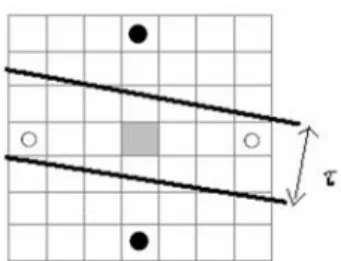
As illustrated in Fig. 2-7, each square represents one pixel and the central one drawn in gray is a candidate pixel. Assuming that white lines are typically no wider than τ pixels (τ = 6 in our system), we check the brightness of the four pixels, marked ‘●’ and ‘○’, at a distance of τ pixels away from the candidate pixel on the four directions. The central candidate pixel is identified as a white line pixel only if both pixels marked ‘●’ or both pixels marked ‘○’ are with lower brightness than the candidate pixel. This process prevents most of the pixels in white regions or white uniforms being detected as white line pixels, as shown in Fig. 2-8 (b).

Fig. 2-7. Illustration of part of an image containing a white line.

(a) Original frame

(b) Without line-structure constraint

(c) With line-structure constraint

Fig. 2-8. Sample results of white line pixel detection.

To improve the accuracy and efficiency of the subsequent Hough transform for line detection and court model fitting, we apply the line-structure constraint [25] to exclude the white pixels in finely textured regions. The structure matrix S [27] computed over a small window of size 2b+1 (we use b=2) around each candidate pixel (px, py), as defined in Eq. (2-4), is used to recognize texture regions.

∑ ∑

+ − = + − =

∇

⋅

∇

=

p b b p x b p b p y T x x y y

y

x

Y

y

x

Y

S

(

,

)

(

(

,

))

(2-4)

classified into textured (λ1, λ2 are large), linear (λ1 » λ2) and flat (λ1, λ2 are small). On the

straight court lines, the linear case will apply to retain the white pixels only if λ1 > αλ2 (α = 4

in our system). Fig. 2-8 demonstrates sample results of white line pixel detection. The original frames are presented in Fig. 2-8(a). In Fig. 2-8(b), although most of the white pixels in white regions or white uniforms are discarded, there are still many false detections of white line pixels occurring in the textured areas. With line-structure constraint, Fig. 2-8(c) shows that the number of false detections is reduced and white line pixel candidates are retained only if the pixel neighbor shows a linear structure.

2.4.2 Line extraction

To extract the court lines and the backboard border, we perform a standard Hough transform on the detected white line pixels. The parameter space (θ, d) is used to represent the line: θ is the angle between the line normal and the horizontal axis, and d is the distance of the line to the origin. We construct an accumulator matrix for all (θ, d) and sample the accumulator matrix at a resolution of one degree for θ and one pixel for d. Since a line in (x, y) space corresponds to a point in (θ, d) space, line candidates can be determined by extracting the local maxima in the accumulator matrix. The court line intersections on the court plane can be obtained by the algorithm of finding line-correspondences in [25], which has good performance in 2D-to-2D court model mapping. A sample result is presented in Fig. 2-9 (a).

To reconstruct 3D information of the ball movement, we need two more points which are not on the court plane to calculate the calibration parameters. The two endpoints of the backboard top-border (p7 and p8 as shown in Fig. 2-6) are selected because the light condition makes the white line pixels of the backboard top-border easy to detect in frames. Fig. 2-9 presents the process of the detection of backboard top-border. In 3D real world, the backboard top-border is parallel with the court lines (p1, p3, p5) and (p2, p4, p6). According to

vanishing point theorem, parallel lines in 3D space viewed in a 2D frame appear to meet at a point, called vanishing point. Therefore, the lines (p1, p3, p5), (p2, p4, p6) and the backboard top- border in the fame will meet at the vanishing point. Utilizing this characteristic, the vanishing point pv can be computed as the intersection of the extracted court lines (p1, p3, p5) and (p2, p4, p6), as shown in Fig. 2-9(b). Besides, we also detect two vertical line segments above the court line (p1, p3, p5). Then, Hough transform is performed on the area between the two vertical lines above the court line (p1, p3, p5). The detected line segment whose extension passes the vanishing point is extracted as the backboard top-boarder, as shown in Fig. 2-9(c).

(a) Detected court lines (b) Computing vanishing point (c) Searching backboard top-border

Fig. 2-9. Detection of backboard top-border.

2.4.3 Computation of camera calibration parameters

Multiplying out the linear system in Eq. (2-3), we obtain two equations, Eq. (2-5) and Eq. (2-6), for each corresponding point—the point whose coordinate is both known in the 3D court model (x, y, z) and in the frame (u′, v′).

c11 x + c12 y + c13 z + c14 = u′ (c31 x + c32 y + c33 z + 1) (2-5) c21 x + c22 y + c23 z + c24 = v′ (c31 x + c32 y + c33 z + 1) (2-6) To compute the calibration parameters cij, we set up a linear system AC = B from Eq. (2-5) and Eq. (2-6):

(2-7) N is the number of corresponding points. In our process, N = 8: six are the court line intersections and two are the endpoints of the backboard top-border. To solve C, we can over-determine A and find a least squares fitting for C with a pseudo-inverse solution:

AC = B, ATAC =ATB, C = (ATA)-1 ATB (2-8)

Thus, the parameters of camera calibration can be derived to form the matrix which transforms 3D real world coordinate to 2D image coordinate.

2.5 2D Shooting Trajectory Extraction

The ball is the most important focus of attention in basketball either for the players or for the audience. It is a challenging task to identify the ball in video frames due to its small size in court views and its fast movement. In this section, we aim at extracting the shooting trajectories in court shots. When a shooting event occurs, one of the backboards should be captured in the frames. Therefore, our system performs ball candidate detection and ball tracking on the frames with a backboard detected in court shots.

2.5.1 Ball candidate detection

The detection of ball candidates, the basketball-colored moving objects, requires extracting the pixels which are 1) moving and 2) in basketball color. For moving pixel

detection, frame difference is a compute-easy and effective method. We extract the pixels with significant luminance difference between consecutive frames as moving pixels. Color is another important feature to extract ball pixels. However, the color of the basketball in frames might vary due to the different angles of view and lighting conditions. To obtain the color distribution of the basketball in video frames, 30 ball images are segmented manually from different basketball videos to produce the respective color histograms in RGB, YCbCr and HSI color spaces, as shown in Fig. 2-10. After statistical analysis, the Hue value in HSI space has better discriminability and is selected as the color feature and the ball color range is set to [Ha, Hb]. We compute the average Hue value for each 4x4 block in frames and discard the

moving pixels in the blocks of which the average Hue values are not within the ball color range [Ha, Hb]. To remove noises and gaps, morphological operations are performed on the

remaining moving pixels, called ball pixels. An example of ball pixel detection is shown in Fig. 2-11. Fig. 2-11(a) is the original frame and Fig. 2-11(b) shows the moving pixels detected by frame difference. The extracted ball pixels after morphological operations are presented in Fig. 2-11(c).

(a) Source frame (b) Moving pixels (c) Extracted ball pixels

Fig. 2-11. Illustration of ball pixel detection.

With the extracted ball pixels, objects are formed in each frame by region growing. To prune non-ball objects, we design two sieves based on visual properties:

1) Shape sieve: The ball in frames might have a shape different from a circle, but the

deformation is not so dramatic that its aspect ratio should be within the range [1/Ra, Ra] in most frames. We set Ra = 3 since the object with aspect ratio > 3 or < 1/3 is far from a ball and should be eliminated.

2) Size sieve: The in-frame ball diameter Dfrm can be proportionally estimated from the length between the court line intersections by pinhole camera imaging principal, as Eq. (2-9):

(Dfrm / Dreal) = (Lfrm / Lreal) , Dfrm = Dreal (Lfrm / Lreal) (2-9) where Dreal is the diameter of a real basketball (≈ 24cm), Lfrm and Lreal are the in-frame length and the real-world length of a corresponding line segment, respectively. To compute the ratio (Lfrm / Lreal), we select the two points closest to the frame center from the six court line intersections and calculate the in-frame distance Lfrm of the selected two points. Since the distance of the two points in real court Lreal is specified in the basketball rules, the ratio (Lfrm / Lreal) can be computed out. Thus, the planar ball size in the frame can be estimated as π • (Dfrm/2)2. The size sieve filter out the objects of which the sizes are not within the range [π • (Dfrm/2)2 – ∆ , π • (Dfrm/2)2 + ∆], where ∆ is the extension for tolerance toward processing faults.

are two major problems we may confront. The first is that more moving pixels are detected due to the camera motion and therefore more ball candidates might exist. However, our analysis is focused on the shooting trajectories in court shots. To capture and present the large portion of the court, the camera is usually located at a distance from the court. The camera motion is not so violent in court shots except for a rapid camera transition from one half-court to the other, as can be noted in Fig. 2-12, where the left image shows the detected ball candidates marked in the yellow circles, and the right image presents the camera motion using motion history image [28], generated from 45 consecutive frames. When a shooting event occurs, one of the backboards should be captured in the frames. During the camera transition since no backboard shows on the screen, our system need not perform ball candidate detection. That is, the performance of ball candidate detection is not affected by the camera moving from one half-court to the other. Second, it is possible (although it is rare in practice) that the ball might have little motion or stay still on the screen when the camera attempts to follow the ball. However, we observe in experiments that the ball is hardly at exactly the same position in consecutive frames even if the camera follows the ball. Although there are still some misses in moving pixel detection in this case due to the mild motion of the ball in frames, the pixels of the true ball can be correctly detected in most frames. The missed ball candidate can be recovered from the ball positions in the previous and the subsequent frames by interpolation.

(a) Fewer ball candidates produced if the camera motion is small.

(b) More ball candidates would be produced if there is large camera motion.

Fig. 2-12. Left: detected ball candidates, marked as yellow circles. Right: motion history

image to present the camera motion.

2.5.2. Ball tracking

Many non-ball objects might look like a ball in video frames and it is difficult to recognize which is the true one. Therefore, we integrate the physical characteristic of the ball motion into a dynamic programming-based route detection mechanism to track the ball candidates, generate potential trajectories and identify the true ball trajectory.

For ball tracking, we need to compute the ball velocity constraint first. Since the displacement of the ball in a long shoot would be larger than that in a short shoot, we take a long shoot into consideration, as diagramed in Fig. 2-13. The time duration from the ball leaving the hand to the ball reaching the peak in the trajectory t1 and the time duration of the ball moving from the peak to the basket t2 can be represented by Eq. (2-10) and Eq. (2-11), respectively:

H+h = g t12 /2 , t1 = [2(H+h)/g]1/2 (2-10) H = g t22 /2 , t2 = (2H/g)1/2 (2-11) where g is the gravity acceleration (9.8 m/s2) and t is the time duration, H and h is the vertical distances from the basket to the trajectory peak and to the position of ball leaving the hand, respectively. Thus, the highest vertical velocity Vv of the ball in the trajectory should be Vv = g t1 and the horizontal velocity Vh can be calculated as Vh = Dis / (t1+t2), where Dis is the distance from the shooter to the basket center. With the vertical and horizontal velocities, the ball velocity Vb can be derived as Eq. (2-12):

Vb = (Vh2+ Vv2)1/2 (2-12) Vb value increases as Dis increases. Since our goal is to compute the upper limit of the ball velocity, we consider the distance from the 3-point line to the basket (6.25m), which is almost the longest horizontal distance from the shooter to the basket. To cover all cases, we set Dis = 7m. Considering an l meter tall player, the height of the ball leaving the hand should be higher than (l+0.2) m. Thus, the value h should be less than (3.05−0.2−l) m. To cover most players, we set l = 1.65, that is, h ≤ 1.2. Besides, there are few shooting trajectories with the vertical distance H greater than 4 meters. Given different h values (0, 0.3, 0.6, 0.9 and 1.2), the values of Vb computed using Eq. (2-10)-(2-12) for H varying between 1 and 4 meters are plotted in Fig. 2-14, showing the reasonable values of Vb. It can be observed that, when H = 4 m and h = 1.2 m, we have the maximum value of Vb (≈ 10.8 m/s). Thus, we set the velocity constraint (upper limit) as Vb ≈ 10.8 m/s ≈ 36 cm/frm. Finally, similar to Eq. (2-9), the in-frame velocity constraint Vc can be proportionally estimated by applying pinhole camera imaging principle as Eq. (2-13):

Fig. 2-13. Diagram of a long shoot. Fig. 2-14. Relation between Vb an H.

The goal of ball velocity constraint is to determine the search range for ball tracking. To avoid ball missing in ball tracking, what we want to derive is the upper limit of in-frame ball velocity. Hence, although there may be deviation of in-frame ball velocity due to the different relationship between the angle of camera shooting and the angle of player’s shooting, the derived upper limit of ball velocity still significantly improves the computational efficiency and accuracy for ball tracking by setting an appropriate search range.

Fig 2-15 illustrates the ball tracking process. The X and Y axes represent the in-frame coordinates of ball candidates, and the horizontal axis indicates the frame number. The nodes C1, C2, C3 and C4 represent the ball candidates. Initially, for the first frame of a court shot, each ball candidate is considered as the root of a trajectory. For the subsequent frames, we check if any ball candidate can be added to one of the existing trajectories based on the velocity property. The in-frame ball velocity can be computed by Eq. (2-14):

j i i j i j j i t y y x x Velocity → → − + − = 2 2 _{( )} ) ( (2-14)

where i and j are frame indexes, (xi, yi) and (xj, yj) are the coordinates of the ball candidates in frame i and frame j, respectively, and ti → j is the time duration. Trajectories grow by adding the ball candidates in the subsequent frames which satisfy the velocity constraint. Although it is possible that no ball candidate is detected in some frames, the trajectory growing process