and Life-Table Statistics
Eric V. Slud
Mathematics Department
University of Maryland, College Park
°2001 c
Eric V. Slud Statistics Program Mathematics Department
University of Maryland
College Park, MD 20742
Contents
0.1 Preface . . . vi
1 Basics of Probability & Interest 1 1.1 Probability . . . 1
1.2 Theory of Interest . . . 7
1.2.1 Variable Interest Rates . . . 10
1.2.2 Continuous-time Payment Streams . . . 15
1.3 Exercise Set 1 . . . 16
1.4 Worked Examples . . . 18
1.5 Useful Formulas from Chapter 1 . . . 21
2 Interest & Force of Mortality 23 2.1 More on Theory of Interest . . . 23
2.1.1 Annuities & Actuarial Notation . . . 24
2.1.2 Loan Amortization & Mortgage Refinancing . . . 29
2.1.3 Illustration on Mortgage Refinancing . . . 30
2.1.4 Computational illustration in Splus . . . 32
2.1.5 Coupon & Zero-coupon Bonds . . . 35
2.2 Force of Mortality & Analytical Models . . . 37 i
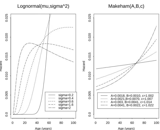
2.2.1 Comparison of Forces of Mortality . . . 45
2.3 Exercise Set 2 . . . 51
2.4 Worked Examples . . . 54
2.5 Useful Formulas from Chapter 2 . . . 58
3 Probability & Life Tables 61 3.1 Interpreting Force of Mortality . . . 61
3.2 Interpolation Between Integer Ages . . . 62
3.3 Binomial Variables & Law of Large Numbers . . . 66
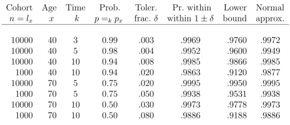
3.3.1 Exact Probabilities, Bounds & Approximations . . . . 71
3.4 Simulation of Life Table Data . . . 74
3.4.1 Expectation for Discrete Random Variables . . . 76
3.4.2 Rules for Manipulating Expectations . . . 78
3.5 Some Special Integrals . . . 81
3.6 Exercise Set 3 . . . 84
3.7 Worked Examples . . . 87
3.8 Useful Formulas from Chapter 3 . . . 93
4 Expected Present Values of Payments 95 4.1 Expected Payment Values . . . 96
4.1.1 Types of Insurance & Life Annuity Contracts . . . 96
4.1.2 Formal Relations among Net Single Premiums . . . 102
4.1.3 Formulas for Net Single Premiums . . . 103
4.1.4 Expected Present Values for m = 1 . . . 104
4.2 Continuous Contracts & Residual Life . . . 106
4.2.1 Numerical Calculations of Life Expectancies . . . 111
4.3 Exercise Set 4 . . . 113
4.4 Worked Examples . . . 118
4.5 Useful Formulas from Chapter 4 . . . 121
5 Premium Calculation 123 5.1 m-Payment Net Single Premiums . . . 124
5.1.1 Dependence Between Integer & Fractional Ages at Death124 5.1.2 Net Single Premium Formulas — Case (i) . . . 126
5.1.3 Net Single Premium Formulas — Case (ii) . . . 129
5.2 Approximate Formulas via Case(i) . . . 132
5.3 Net Level Premiums . . . 134
5.4 Benefits Involving Fractional Premiums . . . 136
5.5 Exercise Set 5 . . . 138
5.6 Worked Examples . . . 142
5.7 Useful Formulas from Chapter 5 . . . 145
6 Commutation & Reserves 147 6.1 Idea of Commutation Functions . . . 147
6.1.1 Variable-benefit Commutation Formulas . . . 150
6.1.2 Secular Trends in Mortality . . . 152
6.2 Reserve & Cash Value of a Single Policy . . . 153
6.2.1 Retrospective Formulas & Identities . . . 155
6.2.2 Relating Insurance & Endowment Reserves . . . 158
6.2.3 Reserves under Constant Force of Mortality . . . 158
6.2.4 Reserves under Increasing Force of Mortality . . . 160
6.2.5 Recursive Calculation of Reserves . . . 162
6.2.6 Paid-Up Insurance . . . 163
6.3 Select Mortality Tables & Insurance . . . 164
6.4 Exercise Set 6 . . . 166
6.5 Illustration of Commutation Columns . . . 168
6.6 Examples on Paid-up Insurance . . . 169
6.7 Useful formulas from Chapter 6 . . . 171
7 Population Theory 161 7.1 Population Functions & Indicator Notation . . . 161
7.1.1 Expectation & Variance of Residual Life . . . 164
7.2 Stationary-Population Concepts . . . 167
7.3 Estimation Using Life-Table Data . . . 170
7.4 Nonstationary Population Dynamics . . . 174
7.4.1 Appendix: Large-time Limit of λ(t, x) . . . 176
7.5 Exercise Set 7 . . . 178
7.6 Population Word Problems . . . 179
8 Estimation from Life-Table Data 185 8.1 General Life-Table Data . . . 186
8.2 ML Estimation for Exponential Data . . . 188
8.3 MLE for Age Specific Force of Mortality . . . 191
8.3.1 Extension to Random Entry & Censoring Times . . . . 193
8.4 Kaplan-Meier Survival Function Estimator . . . 194
8.5 Exercise Set 8 . . . 195
8.6 Worked Examples . . . 195
9 Risk Models & Select Mortality 197
9.1 Proportional Hazard Models . . . 198
9.2 Excess Risk Models . . . 201
9.3 Select Life Tables . . . 202
9.4 Exercise Set 9 . . . 204
9.5 Worked Examples . . . 204
10 Multiple Decrement Models 205 10.1 Multiple Decrement Tables . . . 206
10.2 Death-Rate Estimators . . . 209
10.2.1 Deaths Uniform within Year of Age . . . 209
10.2.2 Force of Mortality Constant within Year of Age . . . . 210
10.2.3 Cause-Specific Death Rate Estimators . . . 210
10.3 Single-Decrement Tables and Net Hazards of Mortality . . . . 212
10.4 Cause-Specific Life Insurance Premiums . . . 213
10.5 Exercise Set 10 . . . 213
10.6 Worked Examples . . . 214 11 Central Limit Theorem & Portfolio Risks 215
13 Bibliography 217
Solutions & Hints 219
0.1 Preface
This book is a course of lectures on the mathematics of actuarial science. The idea behind the lectures is as far as possible to deduce interesting material on contingent present values and life tables directly from calculus and common- sense notions, illustrated through word problems. Both the Interest Theory and Probability related to life tables are treated as wonderful concrete appli- cations of the calculus. The lectures require no background beyond a third semester of calculus, but the prerequisite calculus courses must have been solidly understood. It is a truism of pre-actuarial advising that students who have not done really well in and digested the calculus ought not to consider actuarial studies.
It is not assumed that the student has seen a formal introduction to prob- ability. Notions of relative frequency and average are introduced first with reference to the ensemble of a cohort life-table, the underlying formal random experiment being random selection from the cohort life-table population (or, in the context of probabilities and expectations for ‘lives aged x’, from the subset of lx members of the population who survive to age x). The cal- culation of expectations of functions of a time-to-death random variables is rooted on the one hand in the concrete notion of life-table average, which is then approximated by suitable idealized failure densities and integrals. Later, in discussing Binomial random variables and the Law of Large Numbers, the combinatorial and probabilistic interpretation of binomial coefficients are de- rived from the Binomial Theorem, which the student the is assumed to know as a topic in calculus (Taylor series identification of coefficients of a poly- nomial.) The general notions of expectation and probability are introduced, but for example the Law of Large Numbers for binomial variables is treated (rigorously) as a topic involving calculus inequalities and summation of finite series. This approach allows introduction of the numerically and conceptually useful large-deviation inequalities for binomial random variables to explain just how unlikely it is for binomial (e.g., life-table) counts to deviate much percentage-wise from expectations when the underlying population of trials is large.
The reader is also not assumed to have worked previously with the The- ory of Interest. These lectures present Theory of Interest as a mathematical problem-topic, which is rather unlike what is done in typical finance courses.
Getting the typical Interest problems — such as the exercises on mortgage re- financing and present values of various payoff schemes — into correct format for numerical answers is often not easy even for good mathematics students.
The main goal of these lectures is to reach — by a conceptual route — mathematical topics in Life Contingencies, Premium Calculation and De- mography not usually seen until rather late in the trajectory of quantitative Actuarial Examinations. Such an approach can allow undergraduates with solid preparation in calculus (not necessarily mathematics or statistics ma- jors) to explore their possible interests in business and actuarial science. It also allows the majority of such students — who will choose some other av- enue, from economics to operations research to statistics, for the exercise of their quantitative talents — to know something concrete and mathematically coherent about the topics and ideas actually useful in Insurance.
A secondary goal of the lectures has been to introduce varied topics of applied mathematics as part of a reasoned development of ideas related to survival data. As a result, material is included on statistics of biomedical studies and on reliability which would not ordinarily find its way into an actuarial course. A further result is that mathematical topics, from differen- tial equations to maximum likelihood estimators based on complex life-table data, which seldom fit coherently into undergraduate programs of study, are
‘vertically integrated’ into a single course.
While the material in these lectures is presented systematically, it is not separated by chapters into unified topics such as Interest Theory, Probability Theory, Premium Calculation, etc. Instead the introductory material from probability and interest theory are interleaved, and later, various mathemat- ical ideas are introduced as needed to advance the discussion. No book at this level can claim to be fully self-contained, but every attempt has been made to develop the mathematics to fit the actuarial applications as they arise logically.
The coverage of the main body of each chapter is primarily ‘theoretical’.
At the end of each chapter is an Exercise Set and a short section of Worked Examples to illustrate the kinds of word problems which can be solved by the techniques of the chapter. The Worked Examples sections show how the ideas and formulas work smoothly together, and they highlight the most important and frequently used formulas.
Chapter 1
Basics of Probability and the Theory of Interest
The first lectures supply some background on elementary Probability Theory and basic Theory of Interest. The reader who has not previously studied these subjects may get a brief overview here, but will likely want to supplement this Chapter with reading in any of a number of calculus-based introductions to probability and statistics, such as Larson (1982), Larsen and Marx (1985), or Hogg and Tanis (1997) and the basics of the Theory of Interest as covered in the text of Kellison (1970) or Chapter 1 of Gerber (1997).
1.1 Probability, Lifetimes, and Expectation
In the cohort life-table model, imagine a number l0 of individuals born simultaneously and followed until death, resulting in data dx, lx for each age x = 0, 1, 2, . . ., where
lx= number of lives aged x (i.e. alive at birthday x ) and
dx = lx− lx+1 = number dying between ages x, x + 1
Now, allowing the age-variable x to take all real values, not just whole numbers, treat S(x) = lx/l0 as a piecewise continuously differentiable non-
1
increasing function called the “survivor” or “survival” function. Then for all positive real x, S(x) − S(x + t) is the fraction of the initial cohort which fails between time x and x + t, and
S(x) − S(x + t)
S(x) = lx− lx+t lx
denotes the fraction of those alive at exact age x who fail before x + t.
Question: what do probabilities have to do with the life table and survival function ?
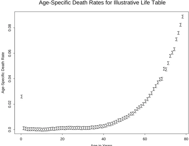
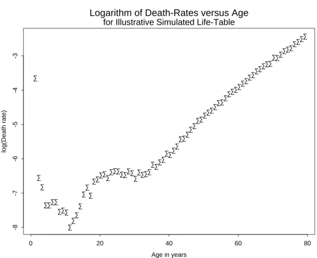
To answer this, we first introduce probability as simply a relative fre- quency, using numbers from a cohort life-table like that of the accompanying Illustrative Life Table. In response to a probability question, we supply the fraction of the relevant life-table population, to obtain identities like
P r(life aged 29 dies between exact ages 35 and 41 or between 52 and 60 )
= S(35) − S(41) + S(52) − S(60) = n
(l35− l41) + (l52− l60)o.
l29
where our convention is that a life aged 29 is one of the cohort surviving to the 29th birthday.
The idea here is that all of the lifetimes covered by the life table are understood to be governed by an identical “mechanism” of failure, and that any probability question about a single lifetime is really a question concerning the fraction of those lives about which the question is asked (e.g., those alive at age x) whose lifetimes will satisfy the stated property (e.g., die either between 35 and 41 or between 52 and 60). This “frequentist” notion of probability of an event as the relative frequency with which the event occurs in a large population of (independent) identical units is associated with the phrase “law of large numbers”, which will bediscussed later. For now, remark only that the life table population should be large for the ideas presented so far to make good sense. See Table 1.1 for an illustration of a cohort life-table with realistic numbers.
Note: see any basic probability textbook, such as Larson (1982), Larsen and Marx (1985), or Hogg and Tanis (1997) for formal definitions of the notions of sample space, event, probability, and conditional probability. The main ideas which are necessary to understand the discussion so far are really
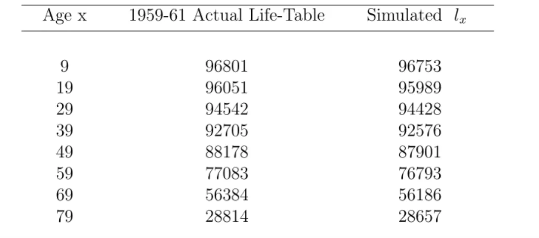
Table 1.1: Illustrative Life-Table, simulated to resemble realistic US (Male) life-table. For details of simulation, see Section 3.4 below.
Age x lx dx x lx dx
0 100000 2629 40 92315 295
1 97371 141 41 92020 332
2 97230 107 42 91688 408
3 97123 63 43 91280 414
4 97060 63 44 90866 464
5 96997 69 45 90402 532
6 96928 69 46 89870 587
7 96859 52 47 89283 680
8 96807 54 48 88603 702
9 96753 51 49 87901 782
10 96702 33 50 87119 841
11 96669 40 51 86278 885
12 96629 47 52 85393 974
13 96582 61 53 84419 1082
14 96521 86 54 83337 1088
15 96435 105 55 82249 1213
16 96330 83 56 81036 1344
17 96247 125 57 79692 1423
18 96122 133 58 78269 1476
19 95989 149 59 76793 1572
20 95840 154 60 75221 1696
21 95686 138 61 73525 1784
22 95548 163 62 71741 1933
23 95385 168 63 69808 2022
24 95217 166 64 67786 2186
25 95051 151 65 65600 2261
26 94900 149 66 63339 2371
27 94751 166 67 60968 2426
28 94585 157 68 58542 2356
29 94428 133 69 56186 2702
30 94295 160 70 53484 2548
31 94135 149 71 50936 2677
32 93986 152 72 48259 2811
33 93834 160 73 45448 2763
34 93674 199 74 42685 2710
35 93475 187 75 39975 2848
36 93288 212 76 37127 2832
37 93076 228 77 34295 2835
38 92848 272 78 31460 2803
39 92576 261
matters of common sense when applied to relative frequency but require formal axioms when used more generally:
• Probabilities are numbers between 0 and 1 assigned to subsets of the entire range of possible outcomes (in the examples, subsets of the in- terval of possible human lifetimes measured in years).
• The probability P (A ∪ B) of the union A ∪ B of disjoint (i.e., nonoverlapping) sets A and B is necessarily the sum of the separate probabilities P (A) and P (B).
• When probabilities are requested with reference to a smaller universe of possible outcomes, such as B = lives aged 29, rather than all members of a cohort population, the resulting conditional probabilities of events A are written P (A | B) and calculated as P (A ∩ B)/P (B), where A ∩ B denotes the intersection or overlap of the two events A, B.
• Two events A, B are defined to be independent when P (A ∩ B) = P (A)·P (B) or — equivalently, as long as P (B) > 0 — the conditional probability P (A|B) expressing the probability of A if B were known to have occurred, is the same as the (unconditional) probability P (A).
The life-table data, and the mechanism by which members of the popula- tion die, are summarized first through the survivor function S(x) which at integer values of x agrees with the ratios lx/l0. Note that S(x) has values between 0 and 1, and can be interpreted as the probability for a single indi- vidual to survive at least x time units. Since fewer people are alive at larger ages, S(x) is a decreasing function of x, and in applications S(x) should be piecewise continuously differentiable (largely for convenience, and because any analytical expression which would be chosen for S(x) in practice will be piecewise smooth). In addition, by definition, S(0) = 1. Another way of summarizing the probabilities of survival given by this function is to define the density function
f (x) = −dS
dx(x) = −S0(x)
as the (absolute) rate of decrease of the function S. Then, by the funda- mental theorem of calculus, for any ages a < b,
P (life aged 0 dies between ages a and b) = (la− lb)/l0
= S(a) − S(b) = Z b
a (−S0(x)) dx = Z b
a
f (x) dx (1.1) which has the very helpful geometric interpretation that the probability of dying within the interval [a, b] is equal to the area under the curve y = f (x) over the x-interval [a, b]. Note also that the ‘probability’ rule which assigns the integral R
A f (x) dx to the set A (which may be an interval, a union of intervals, or a still more complicated set) obviously satisfies the first two of the bulleted axioms displayed above.
The terminal age ω of a life table is an integer value large enough that S(ω) is negligibly small, but no value S(t) for t < ω is zero. For practical purposes, no individual lives to the ω birthday. While ω is finite in real life-tables and in some analytical survival models, most theoretical forms for S(x) have no finite age ω at which S(ω) = 0, and in those forms ω = ∞ by convention.
Now we are ready to define some terms and motivate the notion of ex- pectation. Think of the age T at which a specified newly born member of the population will die as a random variable, which for present purposes means a variable which takes various values x with probabilities governed by the life table data lx and the survivor function S(x) or density function f (x) in a formula like the one just given in equation (1.1). Suppose there is a contractual amount Y which must be paid (say, to the heirs of that individ- ual) at the time T of death of the individual, and suppose that the contract provides a specific function Y = g(T ) according to which this payment depends on (the whole-number part of) the age T at which death occurs.
What is the average value of such a payment over all individuals whose life- times are reflected in the life-table ? Since dx = lx− lx+1 individuals (out of the original l0 ) die at ages between x and x + 1, thereby generating a payment g(x), the total payment to all individuals in the life-table can be written as
X
x
(lx− lx+1) g(x)
Thus the average payment, at least under the assumption that Y = g(T )
depends only on the largest whole number [T ] less than or equal to T , is P
x(lx− lx+1) g(x) / l0 = P
x(S(x) − S(x + 1))g(x)
= P
x
Rx+1
x f (t) g(t) dt =R∞
0 f (t) g(t) dt )
(1.2) This quantity, the total contingent payment over the whole cohort divided by the number in the cohort, is called the expectation of the random payment Y = g(T ) in this special case, and can be interpreted as the weighted average of all of the different payments g(x) actually received, where the weights are just the relative frequency in the life table with which those payments are received. More generally, if the restriction that g(t) depends only on the integer part [t] of t were dropped , then the expectation of Y = g(T ) would be given by the same formula
E(Y ) = E(g(T )) = Z ∞
0
f (t) g(t) dt
The last displayed integral, like all expectation formulas, can be under- stood as a weighted average of values g(T ) obtained over a population, with weights equal to the probabilities of obtaining those values. Recall from the Riemann-integral construction in Calculus that the integral R f(t)g(t)dt can be regarded approximately as the sum over very small time-intervals [t, t + ∆] of the quantities f (t)g(t)∆, quantities which are interpreted as the base ∆ of a rectangle multiplied by its height f (t)g(t), and the rect- angle closely covers the area under the graph of the function f g over the interval [t, t + ∆]. The term f (t)g(t)∆ can alternatively be interpreted as the product of the value g(t) — essentially equal to any of the values g(T ) which can be realized when T falls within the interval [t, t + ∆] — multiplied by f (t) ∆. The latter quantity is, by the Fundamental Theorem of the Calculus, approximately equal for small ∆ to the area under the function f over the interval [t, t + ∆], and is by definition equal to the probability with which T ∈ [t, t + ∆]. In summary, E(Y ) =R∞
0 g(t)f (t)dt is the average of values g(T ) obtained for lifetimes T within small intervals [t, t + ∆] weighted by the probabilities of approximately f (t)∆ with which those T and g(T ) values are obtained. The expectation is a weighted average because the weights f (t)∆ sum to the integral R∞
0 f (t)dt = 1.
The same idea and formula can be applied to the restricted population of lives aged x. The resulting quantity is then called the conditional
expected value of g(T ) given that T ≥ x. The formula will be different in two ways: first, the range of integration is from x to ∞, because of the resitriction to individuals in the life-table who have survived to exact age x; second, the density f (t) must be replaced by f (t)/S(x), the so-called conditional density given T ≥ x, which is found as follows. From the definition of conditional probability, for t ≥ x,
P (t ≤ T ≤ t + ∆¯
¯
¯ T ≥ x) = P ( [t ≤ T ≤ t + ∆] ∩ [T ≥ x]) P (T ≥ x)
= P (t ≤ T ≤ t + ∆)
P (T ≥ x) = S(t) − S(t + ∆) S(x)
Thus the density which can be used to calculate conditional probabilities P (a ≤ T ≤ b¯
¯
¯ T ≥ x) for x < a < b is
∆→0lim 1
∆P (t ≤ T ≤ t+∆¯
¯
¯ T ≥ x) = lim
∆→0
S(t) − S(t + ∆)
S(x) ∆ = −S0(t)
S(x) = f (t) S(x) The result of all of this discussion of conditional expected values is the for- mula, with associated weighted-average interpretation:
E(g(T )¯
¯
¯ T ≥ x) = 1 S(x)
Z ∞
x
g(t) f (t) dt (1.3)
1.2 Theory of Interest
Since payments based upon unpredictable occurrences or contingencies for in- sured lives can occur at different times, we study next the Theory of Interest, which is concerned with valuing streams of payments made over time. The general model in the case of constant interest is as follows. Compounding at time-intervals h = 1/m , with nominal interest rate i(m), means that a unit amount accumulates to (1 + i(m)/m) after a time h = 1/m. The principal or account value 1+i(m)/m at time 1/m accumulates over the time-interval from 1/m until 2/m, to (1+i(m)/m)·(1+i(m)/m) = (1+i(m)/m)2. Similarly, by induction, a unit amount accumulates to (1 + i(m)/m)n = (1 + i(m)/m)T m after the time T = nh which is a multiple of n whole units of h. In the
limit of continuous compounding (i.e., m → ∞ ), the unit amount com- pounds to eδ T after time T , where the instantaneous annualized nominal interest rate δ = limm i(m) (also called the force of interest) will be shown to exist. In either case of compounding, the actual Annual Percentage Rate or APR or effective interest rate is defined as the amount (minus 1, and multiplied by 100 if it is to be expressed as a percentage) to which a unit compounds after a single year, i.e., respectively as
iAPR = ³
1 + i(m) m
´m
− 1 or eδ− 1
The amount to which a unit invested at time 0 accumulates at the effective interest rate iAPR over a time-duration T (still assumed to be a multiple of 1/m) is therefore
³
1 + iAPR
´T
= ³
1 + i(m) m
´mT
= eδ T
This amount is called the accumulation factor operating over the interval of duration T at the fixed interest rate. Moreover, the first and third expres- sions of the displayed equation also make perfect sense when the duration T is any positive real number, not necessarily a multiple of 1/m.
All the nominal interest rates i(m) for different periods of compounding are related by the formulas
(1 + i(m)/m)m = 1 + i = 1 + iAPR , i(m) = m ©(1 + i)1/m − 1ª (1.4) Similarly, interest can be said to be governed by the discount rates for various compounding periods, defined by
1 − d(m)/m = (1 + i(m)/m)−1 Solving the last equation for d(m) gives
d(m) = i(m)/(1 + i(m)/m) (1.5) The idea of discount rates is that if $1 is loaned out at interest, then the amount d(m)/m is the correct amount to be repaid at the beginning rather than the end of each fraction 1/m of the year, with repayment of the principal of $1 at the end of the year, in order to amount to the same
effective interest rate. The reason is that, according to the definition, the amount 1 − d(m)/m accumulates at nominal interest i(m) (compounded m times yearly) to (1 − d(m)/m) · (1 + i(m)/m) = 1 after a time-period of 1/m.
The quantities i(m), d(m) are naturally introduced as the interest pay- ments which must be made respectively at the ends and the beginnings of successive time-periods 1/m in order that the principal owed at each time j/m on an amount $ 1 borrowed at time 0 will always be $ 1. To define these terms and justify this assertion, consider first the simplest case, m = 1. If $ 1 is to be borrowed at time 0, then the single payment at time 1 which fully compensates the lender, if that lender could alternatively have earned interest rate i, is $ (1 + i), which we view as a payment of
$ 1 principal (the face amount of the loan) and $ i interest. In exactly the same way, if $ 1 is borrowed at time 0 for a time-period 1/m, then the repayment at time 1/m takes the form of $ 1 principal and $ i(m)/m interest. Thus, if $ 1 was borrowed at time 0, an interest payment of
$ i(m)/m at time 1/m leaves an amount $ 1 still owed, which can be viewed as an amount borrowed on the time-interval (1/m, 2/m]. Then a payment of $ i(m)/m at time 2/m still leaves an amount $ 1 owed at 2/m, which is deemed borrowed until time 3/m, and so forth, until the loan of $ 1 on the final time-interval ((m − 1)/m, 1] is paid off at time 1 with a final interest payment of $ i(m)/m together with the principal repayment of $ 1. The overall result which we have just proved intuitively is:
$ 1 at time 0 is equivalent to the stream of m payments of
$ i(m)/m at times 1/m, 2/m, . . . , 1 plus the payment of $ 1 at time 1.
Similarly, if interest is to be paid at the beginning of the period of the loan instead of the end, the interest paid at time 0 for a loan of $ 1 would be d = i/(1 + i), with the only other payment a repayment of principal at time 1. To see that this is correct, note that since interest d is paid at the same instant as receiving the loan of $ 1 , the net amount actually received is 1 − d = (1 + i)−1, which accumulates in value to (1 − d)(1 + i) = $ 1 at time 1. Similarly, if interest payments are to be made at the beginnings of each of the intervals (j/m, (j + 1)/m] for j = 0, 1, . . . , m − 1, with a final principal repayment of $ 1 at time 1, then the interest payments should be d(m)/m. This follows because the amount effectively borrowed
(after the immediate interest payment) over each interval (j/m, (j + 1)/m]
is $ (1 − d(m)/m), which accumulates in value over the interval of length 1/m to an amount (1 − d(m)/m)(1 + i(m)/m) = 1. So throughout the year-long life of the loan, the principal owed at (or just before) each time (j + 1)/m is exactly $ 1. The net result is
$ 1 at time 0 is equivalent to the stream of m payments of $ d(m)/m at times 0, 1/m, 2/m, . . . , (m − 1)/m plus the payment of $ 1 at time 1.
A useful algebraic exercise to confirm the displayed assertions is:
Exercise. Verify that the present values at time 0 of the payment streams with m interest payments in the displayed assertions are respectively
m
X
j=1
i(m)
m (1 + i)−j/m + (1 + i)−1 and
m−1X
j=0
d(m)
m (1 + i)−j/m + (1 + i)−1 and that both are equal to 1. These identities are valid for all i > 0.
1.2.1 Variable Interest Rates
Now we formulate the generalization of these ideas to the case of non-constant instantaneously varying, but known or observed, nominal interest rates δ(t), for which the old-fashioned name would be time-varying force of interest.
Here, if there is a compounding-interval [kh, (k + 1)h) of length h = 1/m, one would first use the instantaneous continuously-compounding interest-rate δ(kh) available at the beginning of the interval to calculate an equivalent annualized nominal interest-rate over the interval, i.e., to find a number rm(kh) such that
³1 + rm(kh) m
´ = ³
eδ(kh)´1/m
= exp³δ(kh) m
´
In the limit of large m, there is an essentially constant principal amount over each interval of length 1/m, so that over the interval [b, b + t), with instantaneous compounding, the unit principal amount accumulates to
m→ ∞lim eδ(b)/meδ(b+h)/m · · · eδ(b+[mt]h)/m
= exp
limm
1 m
[mt]−1
X
k=0
δ(b + k/m)
= exp µZ t
0
δ(b + s) ds
The last step in this chain of equalities relates the concept of continuous compounding to that of the Riemann integral. To specify continuous-time varying interest rates in terms of effective or APR rates, instead of the in- stantaneous nominal rates δ(t) , would require the simple conversion
rAPR(t) = eδ(t)− 1 , δ(t) = ln³
1 + rAPR(t)´
Next consider the case of deposits s0, s1, . . . , sk, . . . , sn made at times 0, h, . . . , kh, . . . , nh, where h = 1/m is the given compounding-period, and where nominal annualized instantaneous interest-rates δ(kh) (with compounding-period h) apply to the accrual of interest on the interval [kh, (k + 1)h). If the accumulated bank balance just after time kh is denoted by Bk , then how can the accumulated bank balance be expressed in terms of sj and δ(jh) ? Clearly
Bk+1 = Bk·³
1 + i(m)(kh) m
´
+ sk+1 , B0 = s0
The preceding difference equation can be solved in terms of successive sum- mation and product operations acting on the sequences sj and δ(jh), as follows. First define a function Ak to denote the accumulated bank bal- ance at time kh for a unit invested at time 0 and earning interest with instantaneous nominal interest rates δ(jh) (or equivalently, nominal rates rm(jh) for compounding at multiples of h = 1/m) applying respectively over the whole compounding-intervals [jh, (j + 1)h), j = 0, . . . , k − 1. Then by definition, Ak satisfies a homogeneous equation analogous to the previous one, which together with its solution is given by
Ak+1 = Ak·³
1 + rm(kh) m
´, A0 = 1, Ak =
k−1
Y
j=0
³1 + rm(jh) m
´
The next idea is the second basic one in the theory of interest, namely the idea of equivalent investments leading to the definition of present value of an income stream/investment. Suppose that a stream of deposits sj accruing
interest with annualized nominal rates rm(jh) with respect to compounding- periods [jh, (j + 1)h) for j = 0, . . . , n is such that a single deposit D at time 0 would accumulate by compound interest to give exactly the same final balance Fn at time T = nh. Then the present cash amount D in hand is said to be equivalent to the value of a contract to receive sj
at time jh, j = 0, 1, . . . , n. In other words, the present value of the contract is precisely D. We have just calculated that an amount 1 at time 0 compounds to an accumulated amount An at time T = nh. Therefore, an amount a at time 0 accumulates to a · An at time T , and in particular 1/An at time 0 accumulates to 1 at time T . Thus the present value of 1 at time T = nh is 1/An . Now define Gk to be the present value of the stream of payments sj at time jh for j = 0, 1, . . . , k. Since Bk was the accumulated value just after time kh of the same stream of payments, and since the present value at 0 of an amount Bk at time kh is just Bk/Ak, we conclude
Gk+1 = Bk+1
Ak+1
= Bk(1 + rm(kh)/m)
Ak(1 + rm(kh)/m) + sk+1
Ak+1
, k ≥ 1 , G0 = s0
Thus Gk+1− Gk= sk+1/Ak+1, and
Gk+1 = s0+
k
X
i=0
si+1 Ai+1
=
k+1
X
j=0
sj Aj
In summary, we have simultaneously found the solution for the accumulated balance Bk just after time kh and for the present value Gk at time 0 :
Gk =
k
X
i=0
si
Ai , Bk = Ak· Gk, k = 0, . . . , n
The intuitive interpretation of the formulas just derived relies on the following simple observations and reasoning:
(a) The present value at fixed interest rate i of a payment of $1 exactly t years in the future, must be equal to the amount which must be put in the bank at time 0 to accumulate at interest to an amount 1 exactly t years later. Since (1 + i)t is the factor by which today’s deposit increases in exactly t years, the present value of a payment of $1 delayed t years is (1 + i)−t. Here t may be an integer or positive real number.
(b) Present values superpose additively: that is, if I am to receive a payment stream C which is the sum of payment streams A and B, then the present value of C is simply the sum of the present value of payment stream A and the present value of payment stream B.
(c) As a consequence of (a) and (b), the present value for constant interest rate i at time 0 of a payment stream consisting of payments sj at future times tj, j = 0, . . . , n must be the summation
n
X
j=0
sj (1 + i)−tj
(d) Finally, to combine present values on distinct time intervals, at pos- sibly different interest rates, remark that if fixed interest-rate i applies to the time-interval [0, s] and the fixed interest rate i0 applies to the time- interval [s, t + s], then the present value at time s of a future payment of a at time t + s is b = a(1 + i0)−t, and the present value at time 0 of a payment b at time s is b (1 + i)−s . The idea of present value is that these three payments, a at time s + t, b = a(1 + i0)−t at time s, and b(1 + i)−s= a (1 + i0)−t(1 + i)−s at time 0 , are all equivalent.
(e) Applying the idea of paragraph (d) repeatedly over successive intervals of length h = 1/m each, we find that the present value of a payment of $1 at time t (assumed to be an integer multiple of h), where r(kh) is the applicable effective interest rate on time-interval [kh, (k + 1)h], is
1/A(t) =
mt
Y
j=1
(1 + r(jh))−h
where A(t) = Ak is the amount previously derived as the accumulation- factor for the time-interval [0, t].
The formulas just developed can be used to give the internal rate of return r over the time-interval [0, T ] of a unit investment which pays amount sk at times tk, k = 0, . . . , n, 0 ≤ tk ≤ T . This constant (effective) interest rate r is the one such that
n
X
k=0
sk
³
1 + r´−tk
= 1
With respect to the APR r , the present value of a payment sk at a time tk time-units in the future is sk· (1 + r)−tk. Therefore the stream of payments sk at times tk, (k = 0, 1, . . . , n) becomes equivalent, for the uniquely defined interest rate r, to an immediate (time-0) payment of 1.
Example 1 As an illustration of the notion of effective interest rate, or in- ternal rate of return, suppose that you are offered an investment option under which a $ 10, 000 investment made now is expected to pay $ 300 yearly for 5 years (beginning 1 year from the date of the investment), and then $ 800 yearly for the following five years, with the principal of $ 10, 000 returned to you (if all goes well) exactly 10 years from the date of the investment (at the same time as the last of the $ 800 payments. If the investment goes as planned, what is the effective interest rate you will be earning on your investment ?
As in all calculations of effective interest rate, the present value of the payment-stream, at the unknown interest rate r = iAP R, must be bal- anced with the value (here $ 10, 000) which is invested. (That is because the indicated payment stream is being regarded as equivalent to bank interest at rate r.) The balance equation in the Example is obviously
10, 000 = 300
5
X
j=1
(1 + r)−j + 800
10
X
j=6
(1 + r)−j + 10, 000 (1 + r)−10 The right-hand side can be simplified somewhat, in terms of the notation x = (1 + r)−5, to
300 1 + r
³ 1 − x 1 − (1 + r)−1
´ + 800x (1 + r)
³ 1 − x 1 − (1 + r)−1
´ + 10000 x2
= 1 − x
r (300 + 800x) + 10000x2 (1.6) Setting this simplified expression equal to the left-hand side of 10, 000 does not lead to a closed-form solution, since both x = (1+r)−5 and r involve the unknown r. Nevertheless, we can solve the equation roughly by ‘tabulating’
the values of the simplified right-hand side as a function of r ranging in increments of 0.005 from 0.035 through 0.075. (We can guess that the correct answer lies between the minimum and maximum payments expressed as a fraction of the principal.) This tabulation yields:
r .035 .040 .045 .050 .055 .060 .065 .070 .075 (1.6) 11485 11018 10574 10152 9749 9366 9000 8562 8320
From these values, we can see that the right-hand side is equal to $ 10, 000 for a value of r falling between 0.05 and 0.055. Interpolating linearly to approximate the answer yields r = 0.050 + 0.005 ∗ (10000 − 10152)/(9749 − 10152) = 0.05189, while an accurate equation-solver (the one in the Splus function uniroot) finds r = 0.05186.
1.2.2 Continuous-time Payment Streams
There is a completely analogous development for continuous-time deposit streams with continuous compounding. Suppose D(t) to be the rate per unit time at which savings deposits are made, so that if we take m to go to
∞ in the previous discussion, we have D(t) = limm→ ∞ ms[mt], where [·]
again denotes greatest-integer. Taking δ(t) to be the time-varying nominal interest rate with continuous compounding, and B(t) to be the accumulated balance as of time t (analogous to the quantity B[mt] = Bk from before, when t = k/m), we replace the previous difference-equation by
B(t + h) = B(t) (1 + h δ(t)) + h D(t) + o(h)
where o(h) denotes a remainder such that o(h)/h → 0 as h → 0.
Subtracting B(t) from both sides of the last equation, dividing by h, and letting h decrease to 0, yields a differential equation at times t > 0 :
B0(t) = B(t) δ(t) + D(t) , A(0) = s0 (1.7) The method of solution of (1.7), which is the standard one from differential equations theory of multiplying through by an integrating factor , again has a natural interpretation in terms of present values. The integrating factor 1/A(t) = exp(−Rt
0 δ(s) ds) is the present value at time 0 of a payment of 1 at time t, and the quantity B(t)/A(t) = G(t) is then the present value of the deposit stream of s0 at time 0 followed by continuous deposits at rate D(t). The ratio-rule of differentiation yields
G0(t) = B0(t)
A(t) − B(t) A0(t)
A2(t) = B0(t) − B(t) δ(t)
A(t) = D(t)
A(t)
where the substitutuion A0(t)/A(t) ≡ δ(t) has been made in the third expression. Since G(0) = B(0) = s0, the solution to the differential equation (1.7) becomes
G(t) = s0+ Z t
0
D(s)
A(s) ds , B(t) = A(t) G(t)
Finally, the formula can be specialized to the case of a constant unit-rate payment stream ( D(x) = 1, δ(x) = δ = ln(1 + i), 0 ≤ x ≤ T ) with no initial deposit (i.e., s0 = 0). By the preceding formulas, A(t) = exp(t ln(1 + i)) = (1 + i)t, and the present value of such a payment stream is
Z T
0 1 · exp(−t ln(1 + i)) dt = 1 δ
³1 − (1 + i)−T´
Recall that the force of interest δ = ln(1 + i) is the limiting value obtained from the nominal interest rate i(m) using the difference-quotient representa- tion:
m→∞lim i(m) = lim
m→∞
exp((1/m) ln(1 + i)) − 1
1/m = ln(1 + i)
The present value of a payment at time T in the future is, as expected, µ
1 + i(m) m
¶−mT
= (1 + i)−T = exp(−δ T )
1.3 Exercise Set 1
The first homework set covers the basic definitions in two areas: (i) prob- ability as it relates to events defined from cohort life-tables, including the theoretical machinery of population and conditional survival, distribution, and density functions and the definition of expectation; (ii) the theory of interest and present values, with special reference to the idea of income streams of equal value at a fixed rate of interest.
(1). For how long a time should $100 be left to accumulate at 5% interest so that it will amount to twice the accumulated value (over the same time period) of another $100 deposited at 3% ?
(2). Use a calculator to answer the following numerically:
(a) Suppose you sell for $6,000 the right to receive for 10 years the amount of $1,000 per year payable quarterly (beginning at the end of the first quar- ter). What effective rate of interest makes this a fair sale price ? (You will have to solve numerically or graphically, or interpolate a tabulation, to find it.)
(b) $100 deposited 20 years ago has grown at interest to $235. The interest was compounded twice a year. What were the nominal and effective interest rates ?
(c) How much should be set aside (the same amount each year) at the beginning of each year for 10 years to amount to $1000 at the end of the 10th year at the interest rate of part (b) ?
In the following problems, S(x) denotes the probability for a newborn in a designated population to survive to exact age x . If a cohort life table is under discussion, then the probability distribution relates to a randomly chosen member of the newborn cohort.
(3). Assume that a population’s survival probability function is given by S(x) = 0.1(100 − x)1/2, for 0 ≤ x ≤ 100.
(a) Find the probability that a life aged 0 will die between exact ages 19 and 36.
(b) Find the probability that a life aged 36 will die before exact age 51.
(4). (a) Find the expected age at death of a member of the population in problem (3).
(b) Find the expected age at death of a life aged 20 in the population of problem (3).
(5). Use the Illustrative Life-table (Table 1.1) to calculate the following probabilities. (In each case, assume that the indicated span of years runs from birthday to birthday.) Find the probability
(a) that a life aged 26 will live at least 30 more years;
(b) that a life aged 22 will die between ages 45 and 55;
(c) that a life aged 25 will die either before age 50 or after the 70’th
birthday.
(6). In a certain population, you are given the following facts:
(i) The probability that two independent lives, respectively aged 25 and 45, both survive 20 years is 0.7.
(ii) The probability that a life aged 25 will survive 10 years is 0.9.
Then find the probability that a life aged 35 will survive to age 65.
(7). Suppose that you borrowed $1000 at 6% APR, to be repaid in 5 years in a lump sum, and that after holding the money idle for 1 year you invested the money to earn 8% APR for the remaining four years. What is the effective interest rate you have earned (ignoring interest costs) over 5 years on the
$1000 which you borrowed ? Taking interest costs into account, what is the present value of your profit over the 5 years of the loan ? Also re-do the problem if instead of repaying all principal and interest at the end of 5 years, you must make a payment of accrued interest at the end of 3 years, with the additional interest and principal due in a single lump-sum at the end of 5 years.
(8). Find the total present value at 5% APR of payments of $1 at the end of 1, 3, 5, 7, and 9 years and payments of $2 at the end of 2, 4, 6, 8, and 10 years.
1.4 Worked Examples
Example 1. How many years does it take for money to triple in value at interest rate i ?
The equation to solve is 3 = (1 + i)t, so the answer is ln(3)/ ln(1 + i), with numerical answer given by
t =
22.52 for i = 0.05 16.24 for i = 0.07 11.53 for i = 0.10
Example 2. Suppose that a sum of $1000 is borrowed for 5 years at 5%, with interest deducted immediately in a lump sum from the amount borrowed,
and principal due in a lump sum at the end of the 5 years. Suppose further that the amount received is invested and earns 7%. What is the value of the net profit at the end of the 5 years ? What is its present value (at 5%) as of time 0 ?
First, the amount received is 1000 (1 − d)5 = 1000/(1.05)5 = 783.53, where d = .05/1.05, since the amount received should compound to precisely the principal of $1000 at 5% interest in 5 years. Next, the compounded value of 783.53 for 5 years at 7% is 783.53 (1.07)5 = 1098.94, so the net profit at the end of 5 years, after paying off the principal of 1000, is $98.94.
The present value of the profit ought to be calculated with respect to the
‘going rate of interest’, which in this problem is presumably the rate of 5%
at which the money is borrowed, so is 98.94/(1.05)5 = 77.52.
Example 3. For the following small cohort life-table (first 3 columns) with 5 age-categories, find the probabilities for all values of [T ], both uncondition- ally and conditionally for lives aged 2, and find the expectation of both [T ] and (1.05)−[T ]−1.
The basic information in the table is the first column lx of numbers surviving. Then dx = lx− lx+1 for x = 0, 1, . . . , 4. The random variable T is the life-length for a randomly selected individual from the age=0 cohort, and therefore P ([T ] = x) = P (x ≤ T < x + 1) = dx/l0. The conditional probabilities given survivorship to age-category 2 are simply the ratios with numerator dx for x ≥ 2 , and with denominator l2 = 65.
x lx dx P ([T ] = x) P ([T ] = x|T ≥ 2) 1.05−x−1
0 100 20 0.20 0 0.95238
1 80 15 0.15 0 0.90703
2 65 10 0.10 0.15385 0.86384
3 55 15 0.15 0.23077 0.82770
4 40 40 0.40 0.61538 0.78353
5 0 0 0 0 0.74622
In terms of the columns of this table, we evaluate from the definitions and formula (1.2)
E([T ]) = 0 · (0.20) + 1 · (0.15) + 2 · (0.10) + 3 · (0.15) + 4 · (0.40) = 2.4
E([T ] | T ≥ 2) = 2 · (0.15385) + 3 · (0.23077) + 4 · (0.61538) = 3.4615 E(1.05−[T ]−1) = 0.95238 · 0.20 + 0.90703 · 0.15 + 0.86384 · 0.10 +
+ 0.8277 · 0.15 + 0.78353 · 0.40 = 0.8497
The expectation of [T ] is interpreted as the average per person in the cohort life-table of the number of completed whole years before death. The quantity (1.05)−[T ]−1 can be interpreted as the present value at birth of a payment of $1 to be made at the end of the year of death, and the final expectation calculated above is the average of that present-value over all the individuals in the cohort life-table, if the going rate of interest is 5%.
Example 4. Suppose that the death-rates qx = dx/lx for integer ages x in a cohort life-table follow the functional form
qx = ½ 4 · 10−4 for 5 ≤ x < 30 8 · 10−4 for 30 ≤ x ≤ 55
between the ages x of 5 and 55 inclusive. Find analytical expressions for S(x), lx, dx at these ages if l0 = 105, S(5) = .96.
The key formula expressing survival probabilities in terms of death-rates qx is:
S(x + 1)
S(x) = lx+1
lx = 1 − qx or
lx = l0 · S(x) = (1 − q0)(1 − q1) · · · (1 − qx−1) So it follows that for x = 5, . . . , 30,
S(x)
S(5) = (1 − .0004)x−5 , lx = 96000 · (0.9996)x−5 so that S(30) = .940446, and for x = 31, . . . , 55,
S(x) = S(30) · (.9992)x−30 = .940446 (.9992)x−30
The death-counts dx are expressed most simply through the preceding expressions together with the formula dx = qxlx .
1.5 Useful Formulas from Chapter 1
S(x) = lx
l0
, dx= lx− lx+1
p. 1
P (x ≤ T ≤ x + k) = S(x) − S(x + k)
S(x) = lx− lx+k lx
p. 2
f (x) = −S0(x) , S(x) − S(x + k) = Z x+t
x
f (t) dt
pp. 4, 5
E³ g(T )¯
¯
¯ T ≥ x
´
= 1
S(x) Z ∞
x
g(t) f (t) dt
p. 7
1 + iAPR = µ
1 + i(m) m
¶m
= µ
1 − d(m) m
¶−m
= eδ
p. 8
Chapter 2
Theory of Interest and Force of Mortality
The parallel development of Interest and Probability Theory topics continues in this Chapter. For application in Insurance, we are preparing to value uncertain payment streams in which times of payment may also be uncertain.
The interest theory allows us to express the present values of certain payment streams compactly, while the probability material prepares us to find and interpret average or expected values of present values expressed as functions of random lifetime variables.
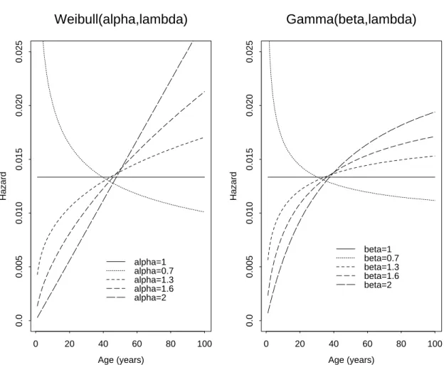
This installment of the course covers: (a) further formulas and topics in the pure (i.e., non-probabilistic) theory of interest, and (b) more discussion of lifetime random variables, in particular of force of mortality or hazard- rates, and theoretical families of life distributions.
2.1 More on Theory of Interest
The objective of this subsection is to define notations and to find compact formulas for present values of some standard payment streams. To this end, newly defined payment streams are systematically expressed in terms of pre- viously considered ones. There are two primary methods of manipulating one payment-stream to give another for the convenient calculation of present
23
values:
• First, if one payment-stream can be obtained from a second one pre- cisely by delaying all payments by the same amount t of time, then the present value of the first one is vt multiplied by the present value of the second.
• Second, if one payment-stream can be obtained as the superposition of two other payment streams, i.e., can be obtained by paying the total amounts at times indicated by either of the latter two streams, then the present value of the first stream is the sum of the present values of the other two.
The following subsection contains several useful applications of these meth- ods. For another simple illustration, see Worked Example 2 at the end of the Chapter.
2.1.1 Annuities & Actuarial Notation
The general present value formulas above will now be specialized to the case of constant (instantaneous) interest rate δ(t) ≡ ln(1 + i) = δ at all times t ≥ 0, and some very particular streams of payments sj at times tj, related to periodic premium and annuity payments. The effective interest rate or APR is always denoted by i, and as before the m-times-per-year equivalent nominal interest rate is denoted by i(m). Also, from now on the standard and convenient notation
v ≡ 1/(1 + i) = 1 / µ
1 + i(m) m
¶m
will be used for the present value of a payment of $1 in one year.
(i) If s0 = 0 and s1 = · · · = snm= 1/m in the discrete setting, where m denotes the number of payments per year, and tj = j/m, then the payment-stream is called an immediate annuity, and its present value Gn
is given the notation a(m)ne and is equal, by the geometric-series summation formula, to
m−1
nm
X
j=1
µ
1 + i(m) m
¶−j
= 1 − (1 + i(m)/m)−nm
m(1 + i(m)/m − 1) = 1 i(m)
³ 1 −³
1 +i(m) m
´−nm´
This calculation has shown
a(m)ne = 1 − vn
i(m) (2.1)
All of these immediate annuity values, for fixed v, n but varying m, are roughly comparable because all involve a total payment of 1 per year.
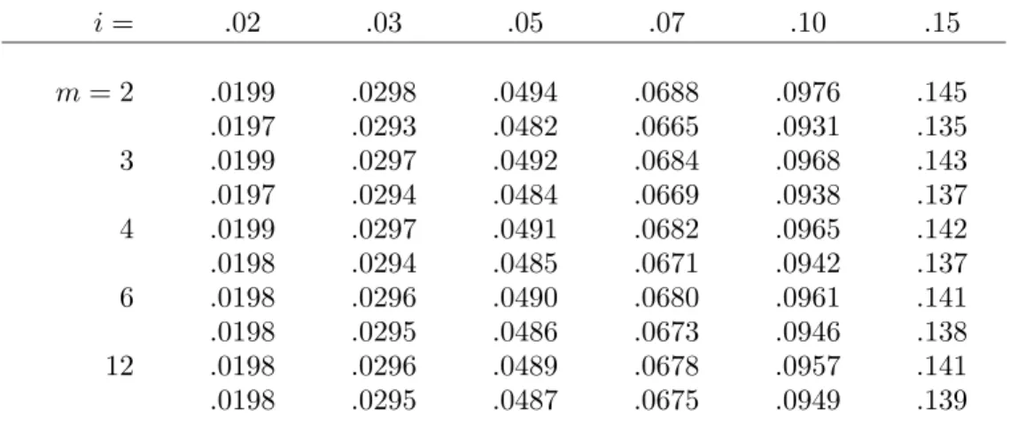
Formula (2.1) shows that all of the values a(m)ne differ only through the factors i(m), which differ by only a few percent for varying m and fixed i, as shown in Table 2.1. Recall from formula (1.4) that i(m) = m{(1 + i)1/m− 1}.
If instead s0 = 1/m but snm = 0, then the notation changes to ¨a(m)ne , the payment-stream is called an annuity-due, and the value is given by any of the equivalent formulas
¨a(m)ne = (1 + i(m)
m ) a(m)ne = 1 − vn
m + a(m)ne = 1
m + a(m)n−1/me (2.2)
The first of these formulas recognizes the annuity-due payment-stream as identical to the annuity-immediate payment-stream shifted earlier by the time 1/m and therefore worth more by the accumulation-factor (1+i)1/m = 1 + i(m)/m. The third expression in (2.2) represents the annuity-due stream as being equal to the annuity-immediate stream with the payment of 1/m at t = 0 added and the payment of 1/m at t = n removed. The final expression says that if the time-0 payment is removed from the annuity-due, the remaining stream coincides with the annuity-immediate stream consisting of nm − 1 (instead of nm) payments of 1/m.
In the limit as m → ∞ for fixed n, the notation ane denotes the present value of an annuity paid instantaneously at constant unit rate, with the limiting nominal interest-rate which was shown at the end of the previous chapter to be limm i(m) = i(∞) = δ. The limiting behavior of the nominal interest rate can be seen rapidly from the formula
i(m) = m³
(1 + i)1/m − 1´
= δ · exp(δ/m) − 1 δ/m
since (ez− 1)/z converges to 1 as z → 0. Then by (2.1) and (2.2), ane = lim
m→∞¨a(m)ne = lim
m→∞a(m)ne = 1 − vn
δ (2.3)
Table 2.1: Values of nominal interest rates i(m) (upper number) and d(m) (lower number), for various choices of effective annual interest rate i and number m of compounding periods per year.
i = .02 .03 .05 .07 .10 .15
m = 2 .0199 .0298 .0494 .0688 .0976 .145
.0197 .0293 .0482 .0665 .0931 .135
3 .0199 .0297 .0492 .0684 .0968 .143
.0197 .0294 .0484 .0669 .0938 .137
4 .0199 .0297 .0491 .0682 .0965 .142
.0198 .0294 .0485 .0671 .0942 .137
6 .0198 .0296 .0490 .0680 .0961 .141
.0198 .0295 .0486 .0673 .0946 .138
12 .0198 .0296 .0489 .0678 .0957 .141
.0198 .0295 .0487 .0675 .0949 .139
A handy formula for annuity-due present values follows easily by recalling that
1 − d(m)
m = ³
1 + i(m) m
´−1
implies d(m) = i(m) 1 + i(m)/m Then, by (2.2) and (2.1),
¨a(m)ne = (1 − vn) · 1 + i(m)/m
i(m) = 1 − vn
d(m) (2.4)
In case m is 1, the superscript (m) is omitted from all of the annuity notations. In the limit where n → ∞, the notations become a(m)∞e and
¨a(m)∞e , and the annuities are called perpetuities (respectively immediate and due) with present-value formulas obtained from (2.1) and (2.4) as:
a(m)∞e = 1
i(m) , ¨a(m)∞e = 1
d(m) (2.5)
Let us now build some more general annuity-related present values out of the standard functions a(m)ne and ¨a(m)ne .
(ii). Consider first the case of the increasing perpetual annuity-due, denoted (I(m)¨a)(m)∞e , which is defined as the present value of a stream of payments (k + 1)/m2 at times k/m, for k = 0, 1, . . . forever. Clearly the present value is
(I(m)¨a)(m)∞e =
∞
X
k=0
m−2(k + 1)³
1 + i(m) m
´−k
Here are two methods to sum this series, the first purely mathematical, the second with actuarial intuition. First, without worrying about the strict justification for differentiating an infinite series term-by-term,
X∞ k=0
(k + 1) xk = d dx
X∞ k=0
xk+1 = d dx
x
1 − x = (1 − x)−2
for 0 < x < 1, where the geometric-series formula has been used to sum the second expression. Therefore, with x = (1 + i(m)/m)−1 and 1 − x = (i(m)/m)/(1 + i(m)/m),
(I(m)¨a)(m)∞e = m−2³ i(m)/m 1 + i(m)/m
´−2
= µ 1
d(m)
¶2
= ³
¨a(m)∞e
´2
and (2.5) has been used in the last step. Another way to reach the same result is to recognize the increasing perpetual annuity-due as 1/m multiplied by the superposition of perpetuities-due ¨a(m)∞e paid at times 0, 1/m, 2/m, . . . , and therefore its present value must be ¨a(m)∞e · ¨a(m)∞e . As an aid in recognizing this equivalence, consider each annuity-due ¨a(m)∞e paid at a time j/m as being equivalent to a stream of payments 1/m at time j/m, 1/m at (j + 1)/m, etc. Putting together all of these payment streams gives a total of (k +1)/m paid at time k/m, of which 1/m comes from the annuity-due starting at time 0, 1/m from the annuity-due starting at time 1/m, up to the payment of 1/m from the annuity-due starting at time k/m.
(iii). The increasing perpetual annuity-immediate (I(m)a)(m)∞e — the same payment stream as in the increasing annuity-due, but deferred by a time 1/m — is related to the perpetual annuity-due in the obvious way
(I(m)a)(m)∞e = v1/m(I(m)¨a)(m)∞e = (I(m)¨a)(m)∞e .
(1 + i(m)/m) = 1 i(m)d(m)
(iv). Now consider the increasing annuity-due of finite duration n years. This is the present value (I(m)¨a)(m)ne of the payment-stream of (k + 1)/m2 at time k/m, for k = 0, . . . , nm − 1. Evidently, this payment- stream is equivalent to (I(m)¨a)(m)∞e minus the sum of n multiplied by an annuity-due ¨a(m)∞e starting at time n together with an increasing annuity- due (I(m)¨a)(m)∞e starting at time n. (To see this clearly, equate the payments 0 = (k + 1)/m2 − n · m1 − (k − nm + 1)/m2 received at times k/m for k ≥ nm.) Thus
(I(m)¨a)(m)ne = (I(m)¨a)(m)∞e
³
1 − (1 + i(m)/m)−nm´
− n¨a(m)∞e (1 + i(m)/m)−nm
= ¨a(m)∞e
³¨a(m)∞e − (1 + i(m)/m)−nmh
¨a(m)∞e + ni ´
= ¨a(m)∞e
³¨a(m)ne − n vn´
where in the last line recall that v = (1 + i)−1 = (1 + i(m)/m)−m and that ¨a(m)ne = ¨a(m)∞e (1 − vn). The latter identity is easy to justify either by the formulas (2.4) and (2.5) or by regarding the annuity-due payment stream as a superposition of the payment-stream up to time n − 1/m and the payment-stream starting at time n. As an exercise, fill in details of a second, intuitive verification, analogous to the second verification in pargraph (ii) above.
(v). The decreasing annuity (D(m)¨a)(m)ne is defined as (the present value of) a stream of payments starting with n/m at time 0 and decreasing by 1/m2 every time-period of 1/m, with no further payments at or after time n. The easiest way to obtain the present value is through the identity
(I(m)¨a)(m)ne + (D(m)¨a)(m)ne = (n + 1 m ) ¨a(m)ne
Again, as usual, the method of proving this is to observe that in the payment- stream whose present value is given on the left-hand side, the payment amount at each of the times j/m, for j = 0, 1, . . . , nm − 1, is
j + 1
m2 + (n
m − j
m2) = 1
m(n + 1 m)