A NETWORK SIMPLEX ALGORITHM FOR SOLVING THE MINIMUM DISTRIBUTION COST PROBLEM

A NETWORK SIMPLEX ALGORITHM FOR SOLVING THE MINIMUM DISTRIBUTION COST PROBLEM

I-Lin Wang and Shiou-Jie Lin

Department of Industrial and Information Management National Cheng Kung University

Tainan, 701, Taiwan

(Communicated by Shu-Cherng Fang)

Abstract. To model the distillation or decomposition of products in some manufacturing processes, a minimum distribution cost problem (MDCP) for a specialized manufacturing network flow model has been investigated. In an MDCP, a specialized node called a D-node is used to model a distillation process that connects with a single incoming arc and several outgoing arcs.

The flow entering a D-node has to be distributed according to a pre-specified ratio associated with each of its outgoing arcs. This proportional relationship between arc flows associated with each D-node complicates the problem and makes the MDCP more difficult to solve than a conventional minimum cost network flow problem. A network simplex algorithm for an uncapacitated MDCP has been outlined in the literature. However, its detailed graphical procedures including the operations to obtain an initial basic feasible solution, to calculate or update the dual variables, and to pivot flows have never been reported. In this paper, we resolve these issues and propose a modified network simplex algorithm including detailed graphical operations in each elementary procedure. Our method not only deals with a capacitated MDCP, but also offers more theoretical insights into the mathematical properties of an MDCP.

1. Introduction. The minimum cost flow problem is a specialized linear program- ming problem with network structure which seeks an optimal flow assignment over a network satisfying the constraints of node flow balance and arc flow bounds (see [1]). However, these constraints are too simplified to model some real cases such as, for example, the synthesis and distillation of products in some manufactur- ing processes. For this purpose, Fang and Qi [8] proposed a generalized network model called the manufacturing network flow (MNF). The MNF considers three specialized nodes: I-nodes, C-nodes, and D-nodes, to model the nodes of inven- tory, synthesis (combination), and distillation (decomposition), in addition to the conventional nodes: S-nodes, T-nodes, and O-nodes, which serve as sources, sinks, and transhipment nodes, respectively. Fang and Qi [8] also defined a minimum distribution cost problem (MDCP) for a specialized MNF model referred to as the distribution network which contains both D-nodes and conventional nodes. A D- node represents a distillation process and only connects with a single incoming arc

2000 Mathematics Subject Classification. Primary: 90B10, 05C85; Secondary: 05C21.

Key words and phrases. network optimization, manufacturing network, distribution network, minimum distribution cost flow problem, network simplex algorithm.

I-Lin Wang was partially supported by the National Science Council of Taiwan under Grant NSC95-2221-E-006-268.

929

M

T

T

T

[0.2]

[0.8]

( object,cost,capacity )

[ material composition percentage ]

(A,3,30)

(A,4,40)

(A,2,40)

(A,5,50) (A,3,30)

(B,3,20)

(C,3,30)

(B,2,20)

(C,4,30)

(B,3,40)

(B,4,10)

(C,3,20)

(B,4,50)

(C,3,30) (A,1,20)

(A,5,50)

d

= the demand of T

d

=10

d

=20

d

=20

[0.2]

[0.8]

(A,5,70)

Figure 1. An MDCP example in a supply chain network

and several outgoing arcs. The flows passing through a D-node have to satisfy the flow distillation constraint. This constraint requires the flows entering a D-node to be distributed to each of its outgoing arcs called distillation arcs, according to a pre-specified ratio associated with each outgoing arc. For each D-node i with enter- ing flow x

on its incoming arc (i

, i), the flow distillation constraint specifies the flow on its distillation arc (i, j) to be x

= k

x

where k

is a constant between 0 and 1 and P

(i,j)

k

= 1.

The MDCP can appear often in part of a supply chain network. Take Figure

as a reverse logistics network example. A recycled product collecting site M distributes a recycled product A which then will be decomposed (or distilled) into materials B and C in two different recycle plants (half-circled nodes), and finally transported to landfills T

, T

, and T

. In this example, each recycle plant is a D-node; M is the S-node; T

, T

, and T

are the T-nodes; and all the other nodes are O-nodes. Suppose that each recycle plant can decompose one unit of A into 0.2 unit of B and 0.8 unit of C. Each arc in the reverse logistics network in Figure

represents some operation (e.g. transportation) associated with a unit cost as well as a capacity constraint. The MDCP in Figure

seeks the minimum possible total cost to satisfy the demand requirements of landfills T

, T

, and T

.

At first glance, the MDCP seems similar to the generalized network flow problem where the flow along an arc (i, j) may lose or gain based on a gain factor µ

, defined as the ratio of the flow arriving at the head node j to the flow leaving from the tail node i. In fact, the generalized flow problem is a special case of the MDCP model. Take Figure

µ

< 1), one may convert it to an MDCP model by adding a dummy sink arc (i, j

) and a D-node α where the flow distillation factors k

and k

can be derived from µ

. Similarly, one may also convert each arc with the gain of flows to an MNF model by adding a dummy source arc and a C-node (see Figure

Besides the generalized flow problem, Cohen and Megiddo [6] also discussed a class

of parametric flow problems in which the fixed ratio flow problem is similar to the

i j i j

i

j'

j i j

i'

α

0.8 0.2

0.8 0.2

α:D-node β

:

(a) flow with loss (b) flow with gain

Figure 2. Converting a generalized flow to the MNF model

MDCP. In particular, the fixed-ratio flow problems have special constraints which are similar to the distillation constraints of the MDCP. Nevertheless, the result in [6] does not help much because of the following two reasons: First, the fixed ratio flow problem can be solved in polynomial time only when the number of those special constraints is a constant, which is more restrictive than MDCP; Second, Cohen and Megiddo [6] only showed the existence of a strongly polynomial algorithm through a sequence of reduction from other problems, rather than providing its detailed operations. Therefore, MDCP is more general and difficult than both the generalized flow problem and the fixed ratio flow problem in the literature.

Although MDCP was defined by Fang and Qi [8], similar problems have been studied by Koene [16], Chen and Engquist [5], and Chang et al. [4] in 1980s. In par- ticular, the pure processing network introduced by Koene [16] also contains nodes of refining, transportation, and blending processes, and is the same as the manufactur- ing network here. Koene [16] showed that any given LP problem can be transformed to a pure processing network problem, and thus can be solved by his specialized primal algorithms. Chen and Engquist [5] proposed basis partitioning techniques in their primal simplex algorithm that used specialized network data structure for the network portion of the problem while treating the other non-network portion as either side variables or constraints. Chang et al. [4] further improved the practical efficiency for the algorithms by Chen and Engquist [5]. Although these previous works also focused on solving MDCPs, their solution methods still involve more alge- braic operations, which are very different from the graphical operations proposed in this paper. Recently, Lu et al. [17] studied the generalized MDCP, where P

(i,j)

k

for all arcs emanating from a D-node i may not necessarily equal to 1. They pro- posed modified network simplex algorithms to deal with min-cost flow problems on a generalized processing network, which has also been previously investigated by Koene [16].

The flow distillation constraints associated with each D-node complicate the

problem and make the MDCP harder than the conventional minimum cost network

flow problem. Although Fang and Qi [8] proposed a network simplex algorithm

for solving the MDCP, their method is, however, not complete in the sense that

it only describes the algebraic structure for a basis. Their proposal lacks details

for the graphical operations such as obtaining the initial solution, and the pivoting

and updating procedures for both the arc flows and node potentials. This paper re- solves these issues and proposes a network simplex algorithm with detailed graphical operations for solving an MDCP.

In addition to the MDCP, Fang and Qi [8] also introduced a max-flow prob- lem for a distribution network, but they did not propose any method to solve the problem. Sheu et al. [19] proposed a multi-labelling method to solve this problem by adopting the concept of the augmenting path method [9] and the Depth-First Search algorithm (DFS) which tries every augmenting subgraph that goes to the sink or source and satisfies the flow distillation constraints. After finding such an augmenting subgraph, the algorithm then identifies decomposable components in an augmenting subgraph where the flow inside each component can be represented by a single variable. The flow can be calculated by the flow balance constraints for all nodes that joint different components. Although this method is straightforward, its complexity is shown to be non-polynomial.

Wang and Lin [21] proposed compacting rules and a polynomial-time compacting algorithm which can serve as a preprocessing procedure to simplify the MDCP problem structure. Specifically, a group of connected D-nodes can be shrunk into a single D-node. Any transhipment O-node with single incoming and outgoing arcs can be transformed into a single arc. Capacities on arcs connecting with a D-node can be unified using the same standards by its flow distillation constraints. After conducting their polynomial-time compacting procedures, the original network will be compacted to an equivalent one of smaller size.

Wang and Yang [22] solved three specialized uncapacitated MDCPs: UMDCP

, UMDCP

, and UMDCP

based on Dijkstra’s algorithm [7]. Other network com- pacting rules which unify the effects of arc costs have also been proposed by the same author. Although two algorithms modified from the Dijkstra’s algorithm have been designed to solve UMDCP

and UMDCP

, they can not efficiently solve UMDCP

. A multicommodity MNF model of σ + 1 commodities was investigated by Mo et al. [18], in which there are σ + 1 layers with each layer corresponding to a network of the same commodity with inter-layer arcs connecting C-nodes or D-nodes. Their model is more restrictive and simplified in the sense that: First, it is assumed that there is only one kind of D-node to decompose commodity 0 into η commodities and one kind of C-node to combine commodity σ from λ commodities; Second, the distillation factor k associated with each D-node (or C-node) is assumed to be identical (i.e. k = 1/η for a D-node, or k = 1/λ for a C-node). Moreover, the elementary procedures in their proposed network simplex algorithm are still pure algebraic rather than graphical operations.

Among all the related literatures, the network-simplex-based solution method by Venkateshan et al. [20] discussed more graphical data structures and operations for solving min-cost MNF problems. Their works are similar to this paper, but their algorithm and notations were not clearly presented. On the other hand, we give more detailed and clear graphical illustration on the theoretical characteristics and complexity for each step of our network simplex algorithm.

In short, several specialized MDCPs have been solved in the literature, yet their

problems are more restrictive (e.g. [18], [21], [22], [19]) or lack graphical operations

(e.g. [16], [5], [4], [8], [18]). Since a network simplex algorithm should contain more

graphical operations than pure algebraic operations like the conventional simplex

algorithm, we propose here in this paper the detailed graphical operations for each

elementary procedure in a network simplex algorithm for solving the MDCP. Our

Figure 3. S-node, T-node, O-node and D-node

work provides a more efficient graphical implementation and more insights into the solution structures. The techniques developed in this paper can also be used to solve the problems in [19] and [22].

The rest of this paper is organized as follows: Section 2 introduces definitions and notations, presents a model transformation for easier illustration, defines a basic feasible graph, and provides optimality conditions for our network simplex algorithm. Detailed procedures of our network simplex algorithm are illustrated in Section 3. Finally, Section 4 summarizes and concludes the paper.

2. Preliminaries.

2.1. Notations and model transformation. Let G = (N, A) be a directed sim- ple graph with node set N and arc set A. For each arc (i, j) ∈ A, we associate it with a unit flow cost c

and a flow capacity u

where the arc flow x

∈ [0, u

].

For each node i ∈ N , we define the set of nodes connecting to and from it as E(i) := {j ∈ N : (j, i) ∈ A} and L(i) := {j ∈ N : (i, j) ∈ A}, respectively. There are four kinds of nodes (see Figure

and they are denoted by N

, N

, N

, and N

, respectively. An S-node is a source node connected only by outgoing arcs. A T-node denotes a sink node connected only by incoming arcs. An O-node represents a transshipment node connected with both incoming and outgoing arcs. Usually, an S-node is a supply node, a T-node is a demand node, and an O-node is for transshipment. We refer to these three types of nodes as conventional nodes since they only have to satisfy the flow balance constraints. A D-node connects with one incoming arc and at least two outgoing arcs. For each node i ∈ N

with incoming arc (i

, i), the flow distillation constraint specifies x

= k

x

for the flow on its distillation arc (i, j). Furthermore, we as- sume P

j∈L(i)

k

= 1 in order to satisfy the flow balance constraint. Without loss of generality, we assume all the networks in this paper to have already been com- pacted using the rules and algorithms by Wang and Lin [21] and Wang and Yang [22]. Also, we assume that the MDCP problem contains a finite optimal solution.

Shipping flows from several S-nodes to several T-nodes through O-nodes and D-nodes, an MDCP model proposed by Fang and Qi [8] is defined as follows:

min X

i∈NS

c

x

+ X

(i,j)∈A

c

x

(MDCP

)

s.t. X

j∈L(i)

x

− x

= 0 ∀i ∈ N

(1)

x

− X

i∈E(j)

x

= 0 ∀j ∈ N

(2)

X

j∈L(i)

x

− x

= 0 ∀i ∈ N

, (i

, i) ∈ A (3) x

− k

x

= 0 ∀i ∈ N

, (i

, i) ∈ A, (i, j) ∈ A (4)

x

≤ u

∀i ∈ N

(5)

0 ≤x

≤ u

∀(i, j) ∈ A (6)

where u

for each i ∈ N

represents the maximum possible flow that a source node i receives for shipping out, d

for each node j ∈ N

denotes the minimum amount of flow that a sink node has to receive, and P

i∈NS

u

≥ P

j∈NT

d

.

Although this formulation is straightforward, it does not follow the conventional notations as they usually appear in the literature of network optimization. For example, x

for each i ∈ N

and x

for each j ∈ N

can not be treated as arc flows since the incoming arc for each S-node and the outgoing arc for each T- node have not been defined in the model. Moreover, each node in a conventional minimum cost network flow model usually has an exact amount of supply or demand, rather than a lower bound (e.g. T-nodes) or upper bound (e.g. S-nodes) as defined in MDCP

. To avoid confusion caused by different notations, we provide the following modifications for MDCP

, based on the modeling techniques proposed in [13,

1. Add a dummy source node s, an arc (s, i) with c

= 0, x

= x

, and u

= u

for each S-node i. Assign P

i∈NS

u

and 0 units of supply for s and each node i ∈ N

, respectively.

2. Add a dummy sink node t, an arc (j, t) with c

= 0, x

= x

− d

, and u

= ∞ for each T-node j. Assign P

i∈NS

u

− P

j∈NT

d

and d

units of demands for t and each node j ∈ N

, respectively.

3. Add the arc (s, t) with c

= 0 and u

= ∞.

Our modification successfully transforms MDCP

into a formulation similar

to the conventional minimum cost network flow model where each node has an

exact amount of supply or demand and each flow variable is associated with an

arc containing both a head node and a tail node. In particular, as illustrated

in Figure

have a fixed amount of net flow. The modified formulation thus contains only

two types of nodes: (1) the D-nodes, and (2) the other nodes denoted as the b O-

nodes, including the original S-nodes, T-nodes, O-nodes, and the dummy nodes s

and t. Let N

= N

∪ N

∪ N

∪ {s, t}, then we update N = N

∪ N

and

A = A ∪ {(s, t)} ∪ {(s, i) : i ∈ N

} ∪ {(j, t) : j ∈ N

}. The new MDCP formulation

after our transformation can be described as follows:

s

i

u

u

i

[ - ]

i i

S

[ -d

]

t

Figure 4. Transforming the MDCP

to the conventional mini- mum cost network flow model

min X

(i,j)∈A

c

x

(MDCP)

s.t. x

+ X

i∈NS

x

= X

i∈NS

u

for s (7)

x

− X

j∈L(i)

x

= 0 ∀i ∈ N

(8)

X

j∈L(i)

x

− X

j∈E(i)

x

= 0 ∀i ∈ N

(9)

x

− X

i∈E(j)

x

= −d

∀j ∈ N

(10)

−x

− X

j∈NT

x

= X

j∈NT

d

− X

i∈NS

u

for t (11)

X

j∈L(i)

x

− X

j∈E(i)

x

= 0 ∀j ∈ N

(12)

k

x

− x

= 0 ∀i ∈ N

, (i

, i) ∈ A, (i, j) ∈ A (13) 0 ≤ x

≤ u

∀(i, j) ∈ A (14) where equations (7) to (12) define the flow balance for each node in N , equation (13) is the flow distillation constraint associated with each D-node, and equation (14) defines the arc flow bounds. Note that we assume P

j∈L(i)

k

= 1 which

means that equation (12) can be derived from equation (13) and thus equation

(12) is removable. This new formulation has several advantages. First, it treats

the MDCP as a side-constrained minimum cost network flow problem where only a new set of flow distillation constraints (i.e. equations (13)) are added in addition to the conventional flow balance and bound constraints; Second, the basic graph corresponding to the basis is connected. Furthermore, the connectivity property of the basic graph is helpful in the development of our network simplex algorithm.

2.2. Basic feasible graph. In a conventional minimum cost network flow prob- lem, a basis corresponds to a spanning tree so that the network simplex algorithm can easily operate from one spanning tree to another. Here in MDCP, the basis corresponding to a basic feasible flow x constitutes a subgraph G

(x) composed by a spanning tree and some distillation arcs. Since the flow balance constraints in MDCP are the same as the conventional minimum cost network flow problem, G

(x) at least contains a spanning tree of n − 1 basic arcs derivable from equations (7) to (12). Suppose each D-node i contains q

distillation arcs, q = P

i∈ND

q

, and that there are a total of p D-nodes. Since equation (12) can be derived from equation (13), we can remove equation (12) and then the rank of the constraints (7) to (13) equals to n + q − p − 1 since there are a total of p D-nodes. The basic feasible graph for an MDCP has the following properties:

Lemma 2.1. Let x be a basic feasible solution of an MDCP and G

(x) be the basic feasible graph corresponding to x, where |N | = n, |N

| = p, |L(i)| = q

for each i ∈ N

and q = P

i∈ND

q

. The basic graph has the following properties:

(i) The number of basic arcs is n + q − p − 1.

(ii) Any cycle of G

(x) includes at least one D-node.

(iii) G

(x) is connected.

(iv) Each D-node i is connected with q

or q

+ 1 basic arcs.

(v) After removing q

− 1 basic arcs for each D-node i, G

(x) can be reduced to a spanning tree.

Proof.

(i) Trivial.

(ii) See [8].

(iii) Our MDCP contains the same flow balance constraints corresponding to a connected spanning tree, as in the conventional minimum cost flow problem. Thus the basic graph of our MDCP is connected.

(iv) See [8].

(v) The proof is modified from [8]. By (iii), we know that any cycle in G

(x) passes at least one D-node. Since each D-node i is connected by at least q

arcs by (iv), and if we remove q

− 1 basic arcs for each D-node i (i.e., totally removing q − p arcs) from G

(x), then the remaining basic graph contains n − 1 basic arcs and remains connected without any cycle which corresponds to a spanning tree.

Although our Lemma

seems similar to the properties proposed by Fang and

Qi [8], they are not identical in the following sense: First, we generalized their

results to deal with a capacitated MDCP whereas their results are only applicable

for an uncapacitated MDCP; Second, we suggest a more specific way (property

(v) in Lemma

(x) and its induced

spanning tree, which helps us to design the optimality conditions in Section 2.3 and

our graphical network simplex algorithm in Section 3.

2.3. Dual variables and optimality conditions. Let π

and ˜ π

be dual variables associated with the flow balance constraint for each node i ∈ N

(equation (7) to (11)) and i ∈ N

(equation (12)), respectively. Let v

denote dual variable associated with the flow distillation constraint (equation (13)) for each distillation arc (i, j). The constraints of the dual problem of an MDCP can be formulated as follows:

π

− π

≤ c

∀i, j ∈ N

(15)

˜

π

− v

− π

≤ c

∀i ∈ N

, j ∈ N

(16) π

− ˜ π

+ X

l∈L(j)

k

v

≤ c

∀j ∈ N

, i ∈ E(j) (17)

For each distillation arc (j, l) leaving D-node j, define ρ

= ˜ π

− v

and π

= P

l∈L(j)

k

ρ

. Since P

l∈L(j)

k

= 1, we will have ˜ π

− P

l∈L(j)

k

v

= P

l∈L(j)

k

(˜ π

− v

) = P

l∈L(j)

k

ρ

= π

. Equation (15) to (17) can be rewritten as π

− π

≤ c

∀i ∈ N

, j ∈ N (18) ρ

− π

≤ c

∀i ∈ N

, j ∈ N

(19) We apply the upper bound technique for linear programming to solve a capac- itated MDCP. Specifically, when x

= u

for an arc (i, j), one may consider its orientation to be reversed. This also means that the check on its dual feasibility constraint has to be conducted conversely (e.g. replace the ≤ with ≥ in equations (18) and (19)). The upper bound technique can also be implemented in the original model proposed by Fang and Qi [8], but their basic graph can not be guaranteed to be connected, which complicates the procedure to traverse along arcs for checking the dual feasibility. On the other hand, the basic graph is shown to be connected in our model by Lemma

Let B, L, and U be the set of basic arcs, non-basic arcs at lower bound, and non-basic arcs at upper bound, respectively. Thus the set of all arcs A = B ∪ L ∪ U . The dual optimality conditions are then as follows:

1. For each arc (i, j) ∈ B,

π

− π

= c

∀i ∈ N

, j ∈ N (20) ρ

− π

= c

∀i ∈ N

, j ∈ N

(21) 2. For each arc (i, j) ∈ L,

π

− π

≤ c

∀i ∈ N

, j ∈ N (22) ρ

− π

≤ c

∀i ∈ N

, j ∈ N

(23) 3. For each arc (i, j) ∈ U ,

π

− π

≥ c

∀i ∈ N

, j ∈ N (24)

ρ

− π

≥ c

∀i ∈ N

, j ∈ N

(25)

3. Network Simplex algorithm. The network simplex algorithm is a specialized

simplex algorithm designed specifically for solving network-type linear programming

problems. The conventional network simplex algorithm is designed for minimum

cost network flow problem and exploits graphical operations in order to efficiently

calculate the basic feasible solutions. However, it cannot deal with the distillation

constraints of an MDCP. On the other hand, the network simplex algorithm pro- posed by Fang and Qi [8] for an MDCP is not complete in the sense that many steps in their algorithm are only algebraic operations. To fully exploit the advantage of graphical operations, we propose a network simplex algorithm including technical details in such steps as to allow us to obtain the initial basic feasible solutions, to pivot flows along basic feasible graphs, and to update dual basic solutions for solving a capacitated MDCP. Without loss of generality, we assume that our MDCP always has a finite optimal solution and that the degeneracy is resolved using anti-cycling techniques. Our network simplex algorithm contains the following steps:

Step 0: Start with an initial basic feasible flow on a basic feasible graph G

(x).

Step 1: Calculate dual basic solutions for G

(x).

Step 2: Check the dual feasibility conditions (equation (22) to (25)) for each arc in L ∪ U . If no arcs violate the optimality conditions, then the flow x is optimal and the algorithm terminates.

Otherwise, select a violating arc (k, l) as the entering arc to the basis and continue Step 3.

Step 3: Conduct flow pivoting operations and determine the leaving arc (v, z).

Step 4: Update dual variables, and then return to Step 2 for the next iteration.

Our algorithm exploits several novel basis partitioning techniques which decom- pose a basic graph into components so that arc flows as well as node potentials can be efficiently calculated and updated. Detailed operations for each step are explained in the next sections.

3.1. Obtaining an initial basic feasible flow. Let M be a very large number.

We present the following procedure based on the Big-M method to compute an initial basic feasible flow:

Step 1: For each i ∈ N

, include arc (s, i) into the basis with x

:= 0. Also include arc (s, t) into the basis with x

:= P

i∈NS

u

− P

i∈NT

d

.

Step 2: For each i ∈ N

, add artificial arcs (s, i) to be a basic arc with u

:= M , c

:= M , and x

:= 0.

Step 3: For each i ∈ N

, add artificial arcs (s, i) to be a basic arc with u

:= M , c

:= M , and x

:= d

.

Step 4: For each i ∈ N

, include each distillation arc (i, j) where j ∈ L(i) to be a basic arc with x

:= 0.

In particular, Step 1 through Step 3 identify n − p − 1 basic arcs, and Step 4 identifies another basic arcs. The flow assignments are feasible since all the supply and demand are satisfied. Furthermore, basic dual variables can be calculated by setting π

:= 0, π

:= −c

for each i ∈ N

, ρ

:= π

+ c

for each distillation arc (i, j), and π

:= P

j∈L(i)

k

ρ

for each i ∈ N

. This procedure takes O(n + q − p) time.

3.2. Calculating basic dual solutions. Fang and Qi [8] outlined this procedure

without detailed graphical implementation. In the present paper we propose a basis

partitioning technique that decomposes the basic graph into p+1 basic components,

in which each basic component is a tree and contains at least one D-node or one

distillation arc. We show that all dual variables on the same basic component can

i

j

j i i

Figure 5. Detaching the distillation from a D-node

be expressed using a representative dual variable (e.g. the π associated with some node in that basic component) due to its tree structure, so that we can use the p + 1 representative dual variables to derive all the n + q dual variables. A system of p + 1 linear equations, composed by π

= ς for some node i ∈ N or ρ

= ς for some distillation arc (α, β) with a constant ς, as well as p equations π

= P

j∈L(i)

k

ρ

of for each i ∈ N

, can be used to solve the p + 1 representative dual variables, and then to derive all the n + q dual variables.

3.2.1. Decomposing the Basic Graph into Basic Components. When solving basic dual variables for a minimum cost network flow problem, the network simplex al- gorithm starts from any node i, sets π

to be a fixed value ς (e.g. ς = 0), and then calculates other dual variables by tracing basic arcs along the basic tree arcs.

Here in MDCP, such a tracing operation is not trivial when a D-node is encoun- tered. Specifically, when starting from a node i ∈ N one may trace along basic arcs and calculate other dual variables π or ρ using equations (20) and (21). However, when a D-node i is encountered, the tracing has to be stopped since the q

+ 1 dual variables in the equation π

= P

j∈L(i)

k

ρ

associated with a D-node i cannot be calculated using a single equation (i.e. equation (20) or (21)). A search algorithm such as the Depth-First Search (DFS) or Breadth-First-Search (BFS) can be used to trace the basic arcs and calculate dual variables using equation (20) and (21), as long as we do not crossover a D-node. Once the search algorithm backtracks to its starting node it can start from any unvisited node and conduct the same operations until all the nodes in N have been visited. That is to say , D-nodes can be viewed as boundary nodes for the search algorithm.

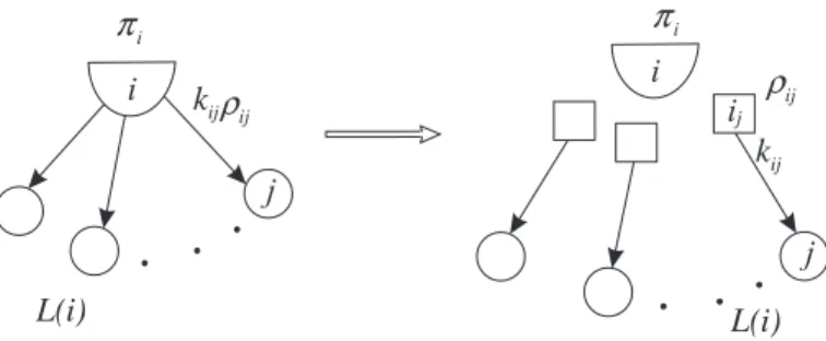
To have a better illustration for this operation, we detach each distillation arc (i, j) outgoing from each D-node i, and replace its tail node by a pseudo node i

referred to as a side-node (the squared nodes in Figure

π

= ρ

is assigned to the side-node i

for recording dual variable ρ

associated with the distillation arc (i, j). Thus equation (21) becomes π

− π

= c

for each distillation basic arc (i, j) and has a form similar to equation (20). Now we only need to consider dual variables π associated with each node in N and each side-node.

The detachment procedure disconnects each D-node i and all the nodes it em- anates to. By lemma

or q

+1 basic arcs. Lemma

−1 basic

arcs for each D-node i in G

(x) reduces the G

(x) to a spanning tree, denoted as

T (x). Therefore, the disconnection of q

basic arcs for each D-node i in G

(x) will

disconnect one more basic arc for each D-node i in the spanning tree T (x). Since

4₇

4₈ 4₆

5₆ 5₉

BC₂ BC₁

BC₃

BC₁

BC₃

BC₂

Figure 6. An example of basic components

there are a total of p D-nodes, the detachment thus disconnects p basic arcs from T (x) and forms a forest of p + 1 trees, where each tree is called a basic component.

Note that each of these p + 1 basic components contains at least one D-node or one side-node.

Since each basic component is a tree, one may arbitrarily choose a node inside a basic component and use its dual variable as a base to derive dual variables along the basic tree arcs for all the other nodes inside the same basic component. Specifically, inside each basic component, the search algorithm starts from a node, sets its dual variable as a base for that basic component, and traverses along basic arcs until it encounters a boundary node (i.e. a D-node or a side-node), then it stops and retreats to visit other unvisited nodes. Whenever a node is visited for the first time, its associated dual variable can be calculated by equation (20) or (21).

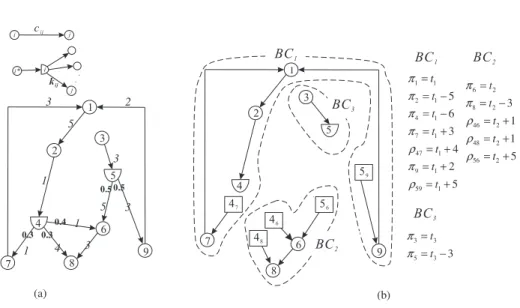
Figure

is decomposed. In this example, three components ( BC

, BC

, and BC

) can be identified, and three independent variables ( π

, π

, and π

) can be used to derive all dual variables through the basic tree arcs.

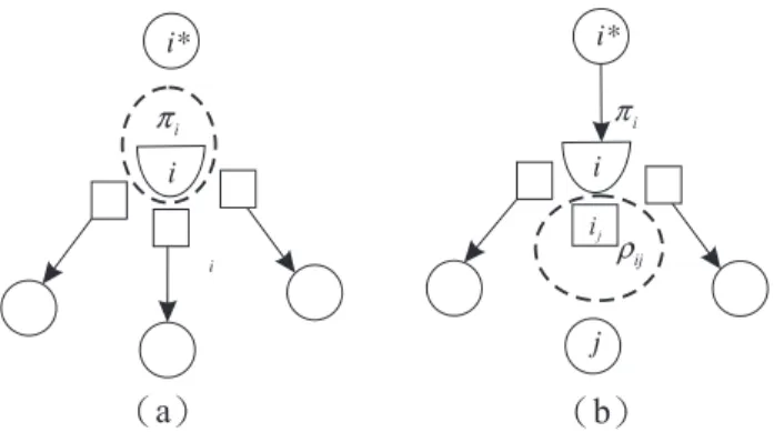
For a D-node i connecting with q

+ 1 basic arcs in G

(x), the detachment will group the D-node i into the basic component containing its entering node i

(i.e.

i

∈ E(i)), while all of its side-nodes belong to the other basic components. On the other hand, for a D-node i connecting with q

basic arcs in G

(x), the detachment will create a basic component composed by an isolated D-node or side-node. For example, Figure

, i) for the D-node i is non-basic, and Figure

the D-node i is non-basic.

Each basic feasible graph can be uniquely decomposed using our basis partition- ing technique. The following are some properties of the basic components.

Lemma 3.1. (i) The number of basic components is p + 1.

(ii) Each basic component is a tree.

(iii) The number of components containing at least one b O-node (i.e. not an isolated

i_j

( ) a ( ) b

Figure 7. Examples of basic components composed by an isolated node

D-node or side-node) is at most min{p + 1, n − p}. That is to say, the number of D-nodes whose adjacent arcs are all basic is at most min{p, n − p − 1}.

Proof.

(i) and (ii) have been explained in previous paragraphs. We give the proof for (iii) as follows:

(iii) If p + 1 ≤ n − p, we may distribute at least one b O-node to each of these p + 1 basic components, so that the maximum number of basic components containing at least one b O-node is p + 1. On the other hand, when p + 1 > n − p, we may at most have n − p among these p + 1 basic components that contain at least one O-node. Therefore, there are at most min{p+1, n−p} basic components containing b at least one b O-node. Since these basic components must be formed by detaching the distillation arcs from those D-nodes whose adjacent arcs are all basic, there are at most min{p, n − p − 1} such D-nodes.

The following are the steps to decompose a basic graph into several basic com- ponents and assign a single variable to express each dual variable in the same component as follows:

Step 0: Given a basic feasible graph G

(x) corresponding to a basic feasible flow x. Construct an augmented basic graph G

(x) by first duplicating all the nodes and arcs from G

(x). Then, for each distillation arc (i, j) in G

(x), detach its tail from the D-node i, and add a new side-node i

vas its new tail node whose dual variable π

= ρ

.

Step 1: Initialize p + 1 node sets ( BC

:= ∅, i = 1, .., p + 1 ); unmark each node (i.e. each node in N and each side-node) in G

(x); set k = 1.

Step 2: Select an unmarked node r from G

(x), put it into BC

, and set π

= t

Step 3: Starting from node r, conduct a search algorithm to traverse along arcs in G

(x). When the search algorithm traverses from a marked node i to an unmarked node j along a basic arc (i, j) (or (j, i) ) in G

(x), we set π

= π

− c

(or π

= π

+ c

). When the search algorithm terminates, all dual variables in this component have been expressed by t

. Set k = k + 1;

Step 4: Repeat Step 2 and Step 3 until all the nodes in G

(x) are marked.

Note that the augmented basic graph G

(x) contains n + q − p − 1 basic arcs and n + q nodes. The search algorithm scans each arc and node exactly once in Step 3 and results in a total θ(n + q) time for this procedure.

3.2.2. Solving a Smaller System of Linear Equations. After decomposing the p + 1 basic components, dual variable associated with each node inside the basic compo- nent has been expressed using the representative variable t

. Thus, there are a total of p + 1 representative dual variables. Similar to the conventional network simplex algorithm for the minimum cost flow problem where one can arbitrarily set a dual variable to a fixed value and then derive all other dual variables with respect to that dual variable via basic arcs, here we can also arbitrarily select a dual variable as a base and compute all other p dual variables accordingly. For example, setting π

= t

= 0, we will have p representative variables (t

: i = 2, ..., p + 1) and a system of p linear equations (π

= P

j∈L(i)

k

ρ

: i ∈ N

).

Take Figure

as an example. Using π

= 0 and the relations between dual variables as defined in Figure

constraints: π

= 0.4ρ

+ 0.3ρ

+ 0.3ρ

and π

= 0.5ρ

+ 0.5ρ

can be expressed using t

and t

, and we can compute t

= −11.286 and t

= 0.5t

+ 8 = 2.357.

Although our basis partitioning technique requires us to solve a system of p linear equations for calculating basic dual variables, this is already more efficient than solving a system of n + q − p − 1 linear equations as required in the network simplex method proposed by Fang and Qi [8]. In fact, the efficiency of our method can be improved further, if a better ordering in the sequence of components to be solved can be identified. For example, in Figure

node for two components (BC

and BC

), and D-node 5 is the boundary node for three components (BC

, BC

, and BC

). Setting t

= 0 will have to solve a 2 × 2 system of linear equations, whereas setting t

= 0 or t

= 0 will make the remaining system of linear equations become a triangular form, which can be solved more efficiently.

To speed up this procedure, we may reduce the number of linear equations re- quired to be solved. We first identify the following three types of basic components:

(1) a basic component composed of an isolated D-node or side-node (e.g. Figure

O-nodes but no side-nodes (e.g. the BC

in Figure

D-node, some b O-nodes, and some side-nodes whose associated distillation arcs are emanating from the same D-node in the adjacent basic component. We call these three types of basic components leaf basic components since their dual variables only depend on a single dual variable without interacting with others. Thus, dual variables inside a leaf basic component can first be left aside, and then later be derived from dual variables of other non-leaf basic components. By Lemma

we know that there are at most min{p + 1, n − p} basic components that are not leaf basic components. Thus, we may at most solve a system of min{p + 1, n − p} linear equations which takes O(min{p

, (n − p)

}) time. Then, the calculation on dual variables in the remaining leaf basic components takes O(p + q) time. In summary, the procedure to calculate all dual variables takes O(min{p

, (n − p)

} + n + q) time.

3.3. Finding an entering arc and pivoting flows. After calculating basic dual

variables, any arc in L ∪ U that violates the dual feasibility conditions (equation

(22) to (25)) is eligible to enter the basis. A pivoting graph, obtained by adding

the entering arc to the basic graph, contains more than one cycle since the original

4

5

entering arc

basic arc

orientation

Figure 8. Pivoting flow inside a basic component

basic graph already contains cycles induced by the D-nodes. Thus the flow pivoting operations become more difficult and complicated. Similar to the computation on dual variables, the difficulty of flow pivoting lies in the design of an efficient procedure to pivot flows graphically, rather than algebraically. To this end, we apply the basis partitioning technique used in calculating dual variables to design efficient graphical flow pivoting operations. There are two types of entering arcs:

either the entering arc connects two nodes of the same component or it does not.

We provide different procedures to conduct flow pivoting for these two cases.

3.3.1. The Entering Arc Connecting Nodes of the Same Basic Component. Since each basic component is a tree, adding the non-basic entering arc (k, l) in this case will induce a unique cycle inside the same basic component, as shown in Figure

In addition, nodes k, l, and other nodes on the induced cycle have to be b O-nodes, since all the D-nodes will become leaf nodes in G

(x) (and thus D-nodes can not become internal nodes). The flow pivoting operations in this case are made up of the following steps:

Step 1: Add the non-basic entering arc (k, l) into the BC containing nodes k and l.

Step 2: Identify the unique cycle induced by adding (k, l) to the BC containing nodes k and l.

Step 3: If (k, l) ∈ L, we ship the maximum flow along the orientation of (k, l) in the induced cycle, Update flows for the arcs in the induced cycle, and then determine the leaving arc (v, z) that first achieves its flow bound.

Otherwise (i.e. (k, l) ∈ U ), we ship the maximum flow along the opposite orientation of (k, l) in the induced cycle, update flows for the arcs in the induced cycle, and then determine the leaving arc (v, z) that first achieves its flow bound.

This procedure takes O(n + q) time.

3.3.2. The Entering Arc Connecting Nodes of Different Basic Components. Three types of end nodes for the entering arc (k, l) are possible in this case: (1) k ∈ N

, l ∈ N

(2) k ∈ N

, l ∈ N

, and (3) k ∈ N

, l ∈ N

. In general, the entering arc merges two components and reduces the number of basic components from p + 1 to p. Note that in this case the entering arc induces no cycle in the newly merged component, and thus we have to design a new graphical procedure to pivot flows.

Here we will exploit the basis partitioning techniques used for calculating basic dual variables in Section 3.2 to compute flows in the pivoting process.

To speed up the calculation, we conduct a graph compacting process to remove those nodes not eligible to ship flows in the pivoting graph, as well as their associated arcs. In particular, two types of nodes are removable: (1) any b O-node connecting with one arc, and (2) any node inside a leaf basic component. This compacting procedure may be repeated until all the b O-nodes are connected with at least two basic arcs and all the leaf basic components are removed. Since each compacting operation removes at least one node and one basic arc, it takes a total of O(n + q) time.

The graph compacting procedure reduces the number of components in a pivoting graph from p to ˜ p. e G = ( e N , e A) denotes the remaining pivoting graph after the compacting process. We give four properties for e G as follows:

Lemma 3.2. (i) Any leaf node in e N is either a D-node or a side node.

(ii) Any D-node i in e N has to be adjacent to q

+ 1 arcs.

(iii) ˜ p ≤ min{p, n − p}.

(iv) e G contains ˜ p D-nodes.

Proof.

(i) and (ii) are trivial since the compacting process removes all the leaf b O- nodes, as well as those isolated D-nodes or side-nodes. We give the proof for (iii) and (iv) as follows:

(iii) If p + 1 ≤ n − p, then we know that p < n − p and thus ˜ p ≤ p since the n − p O-nodes can at most cover all the p components in the pivoting graph. On the other b hand, if p + 1 > n − p, then we know that p ≥ n − p and thus ˜ p ≤ n − p since the n − p b O-nodes can at most cover n − p of the p components in the pivoting graph.

Therefore, ˜ p ≤ min{p, n − p}.

(iv) The ˜ p components have to include the merged basic components induced by the entering arc (k, l), since the entering arc is the source of any flow change. This means that there were ˜ p + 1 basic components if we exclude the entering arc from A. Since these ˜ e p + 1 basic components must be formed by detaching the distillation arcs from the ˜ p D-nodes, and these D-nodes will not be removed by (ii), so we know N contains ˜ e p D-nodes.

To conduct the flow pivoting operation, we have to identify the relationship of flow changes on basic arcs with respect to the flow change on the entering arc. To this end, we first set ∆

= 1 (or ∆

= −1) to represent the shipping of one unit of flow along the entering arc (k, l) if (k, l) ∈ L (or (k, l) ∈ U ), and then for each D-node i we assign the flow change along its incoming arc to be ∆

(thus we have in total ˜ p variables of ∆

by Lemma

balance constraints, we can derive the flow change on each arc in e A in terms of f

for each D-node i. Specifically, the flow in each distillation arc can be derived by

∆

= k

∆

for each D-node i. Since each component in e G is a tree with leaf nodes as D-nodes or side-nodes, all the flow change entering or leaving each leaf node can be expressed by ∆

for each D-node i.

In addition, using the flow balance constraints associated with each internal node, we can conduct a search algorithm inside a component to traverse from leaf nodes to all other internal nodes and derive the flow change entering or leaving each internal node in terms of ∆

for each D-node i. Thus, for each component in e G, we may arbitrarily select an internal node as its root node and use the flow balance equation associated with each root node to construct a system of ˜ p linear equations. Note that this system of ˜ p linear equations has a rank equal to ˜ p − 1 since the flow balance constraints have to be satisfied for each node and for the entire system itself. Thus, one of the ˜ p flow balance equations can be removed. On the other hand, by considering the additional equation ∆

= 1 (or ∆

= −1, depending on whether (k, l) ∈ L or (k, l) ∈ U ) representing the unit flow change for the entering arc (k, l), a system of ˜ p linear equations can be constructed to solve the ˜ p variables of ∆

for each D-node i, and then all the relative flow changes on each arc in e A can be derived with respect to ∆

.

Obtaining the relative flow change for each arc in e A, we can conduct a minimum ratio test to calculate θ

= min

ij6=0

{(u

− x

)/∆

: ∆

> 0, −x

/∆

:

∆

< 0} for a leaving arc (v, z), update flows by x

= x

+ θ

∆

for each arc (i, j) in b A with ∆

6= 0, and then remove (v, z) to form another basic graph for the next iteration.

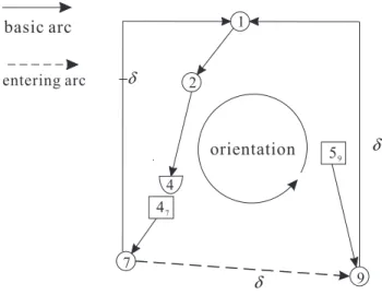
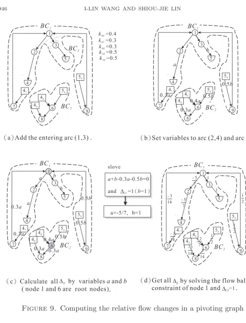
Take the pivoting graph in Figure

it merges two basic components BC

and BC

. Setting the amount of flow changes on arcs and to be a and b, respectively, we may derive the flow changes entering or leaving the leaf nodes, as shown in Figure

the root nodes in BC

and BC

, respectively, we can derive all the flow changes entering or leaving each internal node as shown in Figure

equations, a + b − 0.3a − 0.5b = 0 and −0.3a − 0.4a − 0.5b = 0, associated with these root nodes can be formulated. Since these two equations depend on each other, we replace the second equation by b = 1 since the entering arc (1, 3) ∈ L. Therefore we can derive the flow change for each arc in the pivoting graph relative to the flow change on the entering arc, as shown in Figure

The procedure to pivot the flow in the case where the entering arc connects nodes of different basic components is described as follows:

Step 1: Add the non-basic entering arc (k, l) into G

(x) to construct a pivoting graph.

Step 2: Conduct the graph compacting procedure which repeatedly removes any O-node connecting with one arc and any node inside a leaf basic component, b as well as their associated arcs in a pivoting graph, until no more such node exists. We call the compacted graph as e G = ( e N , e A).

Step 3: For each node i ∈ N

in e N , we assign a flow change variable ∆

for its incoming arc (i

, i), and then calculate ∆

= k

∆

for each distillation arc (i, j).

Step 4: For each component in e G, we select some b O-node in this component as its

root node, conduct a search algorithm to traverse from leaf nodes to the root

( )a Add the entering arc (1,3) . ( )b Set variables to arc (2,4) and arc (3,5).

( )c Calculate all ( )d G

(b=1)

variablesaandb

5 7 -

3 14 -

3 14 -

5 7 -

3 14

- 3

14 2 7

- 1

2 1 2

1 2 1

1

BC₁

BC₂ BC₃

BC₁

BC2

BC1

BC₂ BC₁

BC₂

root

Figure 9. Computing the relative flow changes in a pivoting graph node, and then derive the flow change on any arc inside that component using the flow balance constraints associated with each internal node.

Step 5: If (k, l) ∈ L, we solve the system of equations composed by ∆

= 1 and the flow balance constraints associated with ˜ p − 1 root nodes in e N to obtain

∆

for each (i, j) ∈ e A.

Otherwise (i.e. (k, l) ∈ U ), we solve the system of equations composed by

∆

= −1 and the flow balance constraints associated with ˜ p − 1 root nodes in e N to obtain ∆

for each (i, j) ∈ e A.

Step 6: Calculate θ

= min

ij6=0

{(u

− x

)/∆

: ∆

> 0, −x

/∆

:

∆

< 0} for a leaving arc (v, z).

Step 7: For each arc (i, j) ∈ e A with ∆

6= 0, we update its flow by x

:= x

+ θ

∆

.

The compacting procedure takes O(n + q − p) time to construct e G. Setting the

flow change variables for arcs connecting with D-nodes takes O(˜ p + ˜ q) time, where