1 1
Graduate Institute of Electronics Engineering College of Electrical Engineering & Computer Science
National Taiwan University Master Thesis
50
Architecture Design of Convolutional Neural Networks for Face Detection on FPGA Platforms
Bin-Syh Yu
Advisor: Shao-Yi Chien, Ph.D.
6
June 2016
!
G 0 & .A 01 rco b D n IF
C GD CPl G L
F y GC m PC w x gC S
n e e F G 6
D g at
n a
S
n l i
l C 6 l
C l l G 6 M S
l C a r X D 02 2
02 2 6 GC
D GC
Ss C w
f m n FG f S C iC
F C D d C
e 87 85 387 5 9 5 89 C
w co
CG r A e
C As c CGs
P kN
e gA A vd e
gA % l A a c
t n F
i
A e 5 9 89 co P
3 5 9829 .5 99 u a P
P m
yP b
Architecture Design of
Convolutional Neural Networks for
Face Detection on FPGA Platforms
Bin-Syh Yu
Advisor: Shao-Yi Chien
Graduate Institute of Electronics Engineering National Taiwan University
Taipei, Taiwan, R.O.C.
June 2016
ii
Abstract
Convolutional neural networks (CNNs) have emerged to provide powerful dis- criminative capability, especially in the world of image recognition and object de- tection. However, their massive computation requirements, storage and memory accesses make them hard to be deployed on mobile or embedded systems.
In this thesis, a few optimizations based on a CNN cascade architecture for face detection are proposed to increase throughput while minimizing computation, storage and bandwidth requirement under power constraints.
First, the first net of the CNN cascade is converted to a fully convolutional network to reduce 83% of the computation in the first stage. Second, an efficient method is applied to quantize the model parameters. This is done by adopting a retraining method, reducing the word length of the parameters from 32-bit floating points to 2-bit fixed points, resulting in 93.75% less parameter memory size.
Finally, a CNN accelerator is implemented on a Xilinx XC7020 FPGA board.
We quantitatively analyze the computing throughput and required bandwidth us- ing the roofline model, an analytical design scheme, to find the solution with best performance and lowest FPGA resource requirement. Furthermore, we show that more computational ability benefits from the quantizing optimization.
i
ii
Contents
Abstract i
List of Figures vii
List of Tables ix
1 Introduction 1
1.1 Face Detection . . . 1
1.2 Deep Learning . . . 2
1.2.1 Introduction . . . 2
1.2.2 Output Hypothesis . . . 4
1.2.3 Feedforward Process . . . 4
1.2.4 Backpropagation . . . 5
1.3 Challenges . . . 6
1.4 Thesis Organization . . . 6
2 Face Detection Architecture and Fully Convolutional Networks 7 2.1 Introduction . . . 7
2.2 A CNN Cascade for Face Detection . . . 7
2.2.1 Overall Framework . . . 8
2.2.2 Calibration Nets . . . 9
2.2.3 Training Process . . . 9
2.3 Fully Convolutional Networks . . . 10 iii
iv
2.3.1 Introduction . . . 10
2.3.2 Example . . . 10
2.3.3 Applications . . . 11
2.4 Fully Convolutional Network Version of CNN Cascade . . . 12
2.4.1 Architecture . . . 12
2.4.2 Computation Reduction . . . 14
2.5 Summary . . . 15
3 Quantizing 17 3.1 Introduction . . . 17
3.2 Hard Quantizing . . . 19
3.3 Stochastic Rounding . . . 19
3.4 Modifying the Cost Function . . . 21
3.5 Network Retraining . . . 22
3.6 Summary . . . 23
4 Hardware Implementation 25 4.1 Introduction . . . 25
4.2 Potential Accelerations of a Typical CNN . . . 25
4.3 The Roofline Model . . . 26
4.4 Loop Tiling . . . 27
4.5 Computation Optimization . . . 28
4.5.1 Loop Unrolling . . . 28
4.5.2 Tile Size Selection . . . 30
4.6 CTC Ratio and Benefits from Quantizing . . . 30
4.7 Optimal Parameters . . . 32
4.8 Block Diagram . . . 32
4.9 Computation Engine . . . 33
4.10 Experiments . . . 34
4.10.1 Development Device . . . 34
v 4.10.2 Performance Comparison to CPU . . . 36 4.11 Summary . . . 36
5 Conclusion 37
Reference 39
vi
List of Figures
1.1 The goal of face detection, results should provide the location of each of the faces. [1] . . . 1 1.2 A typical configuration of a convolutional neural network. . . 3 2.1 Testing pipeline from [2]. . . 8 2.2 Calibrated bounding boxes are better aligned to the faces: the blue
rectangles are the most confident detection bounding boxes of 12- net; the red rectangles are the adjusted bounding boxes with the 12-calibration-net. [2]. . . 9 2.3 The architecture of AlexNet [3]. . . 10 2.4 The efficiency of CNNs for detection [4]. . . 11 2.5 Results of feedforwarding an image through the fully convolu-
tional version of AlexNet [5]. . . 12 2.6 Downscaling of an example image. . . 13 2.7 Results of feedforwarding an image through the fully convolu-
tional version of 12-net in the CNN cascade architecture. . . 13 2.8 Images are iteratively downscaled until either side of the image is
smaller than 12 pixels. . . 14 3.1 A quantized neural networks with multiplexers, where the quan-
tized parameters w can only be -1, 0, or +1. . . 18 3.2 Evaluating hard quantized parameters on FDDB . . . 20 3.3 Evaluating stochastically rounded parameters on FDDB . . . 21
vii
viii
3.4 Network retraining proposed in [6] . . . 23
3.5 Evaluating retrained parameters on FDDB . . . 24
4.1 Graph of a convolutional layer [7]. . . 25
4.2 The roofline model [8]. . . 26
4.3 The data sharing relations [8]. . . 29
4.4 Block diagram . . . 33
4.5 Computation Engine [8] . . . 34
4.6 Resources of different Zynq devices [9]. . . 35
List of Tables
3.1 Cell area comparison of a 32-bit floating point multiplier and a 10-bit 3 to 1 multiplexer. . . 18 4.1 Maximum execution cycles under different tile sizes . . . 32 4.2 Performance (GFLOPS) on the second convolutional layer of 48-
net under different tile sizes. . . 35 4.3 Performance comparison to CPU . . . 36
ix
x
Chapter 1 Introduction
1.1 Face Detection
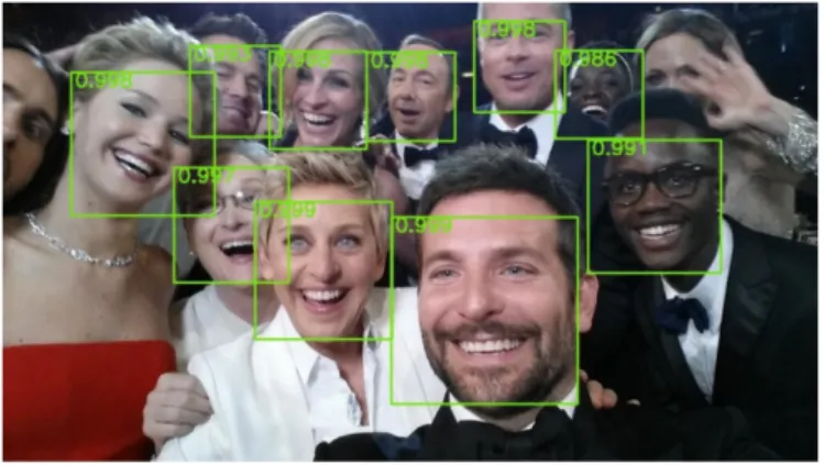
Figure 1.1: The goal of face detection, results should provide the location of each of the faces. [1]
Face detection has been one of the most studied topics in the field of computer vision. Given an image, the goal of face detection is to determine if there are any faces in the given image, and to return the number of faces along with the location of each of the faces, as shown in Fig. 1.1. The main difficulties of face detec- tion come from variations in scale, location, pose, orientation, facial expressions, occlusions, and the massive search space of possible faces in the given image.
1
2
To accomplish such a task, many hand-designed features such as Haar-like features[10], binarized features such as Modified-census transform[11] and LBP features[12, 13], locally assembled binary (LAB) features[14], statistics-based features[15], and composite features[16] have been proposed in the past decades.
Ever since the seminal work of Viola et al.[10], a number of face detectors have been proposed based on such a boosted cascade structure. Due to the rela- tively weak discriminative ability of Haar-like features, the original face detector typically fails in environments where faces have different poses, expressions, and unexpected lighting.
With such observations, it seems that replacing Haar-like features with more advanced features such as Convolutional Neural Networks (CNNs) could achieve even better performance, since the CNNs can automatically learn features to cap- ture visual variations that hand-designed features are incapable of handling.
1.2 Deep Learning
1.2.1 Introduction
In recent years, especially after the representative work of Krizhevsky et al.[3], deep learning has grown rapidly. It has been proven to dramatically surpass pre- vious works in fields including image and video recognition [17], image to text translation [18], speech recognition [19], and text understanding [20].
However, the massive computation requirements, storage and memory ac- cesses required by deep convolutional neural networks make them hard to be deployed on mobile or embedded systems, especially under speed and power con- straints.
A typical deep convolutional neural network model consists of a sequence of layers. There are mainly three types of layers: convolutional layers, pooling layers, and fully-connected layers. These layers are stacked together in a way to form a complete deep CNN model.
3
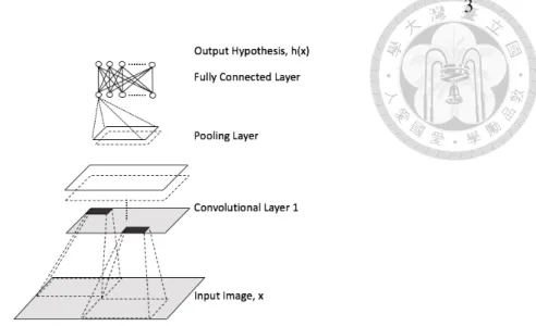
Figure 1.2: A typical configuration of a convolutional neural network.
An example of a deep convolutional neural network is shown in Fig. 1.2, which is composed of convolutional and fully connected layers from the input to the output. State-of-the-art models usually have more layers with more weighting and bias parameters.
In this particular model, the input may be a [32 ⇥32⇥3] image with 32 pixels of width and height, and three color channels R, G, B. The convolutional layer consists of neurons, values that are calculated by performing dot operations with learned weights w on regions of the previous layer and adding a bias value b, producing output feature maps y of, for example, size [30 ⇥ 30 ⇥ 16], assuming there are 16 filters of sizes [3 ⇥ 3 ⇥ 3].
The pooling layer would perform a downscaling operation on the previous convolutional layer, usually in the form of retrieving the maximum or computing the average of neurons in regions. Assuming the stride to be 2 pixels, the resulting output feature map of the pooling layer could be of size [15 ⇥ 15 ⇥ 16].
The fully-connected layer would then be fully connected to the previous layer, performing operations exactly the same as in normal neural networks.
4
1.2.2 Output Hypothesis
For a classification problem, the last output hypothesis usually outputs a vector of elements in the range of (0, 1) that add up to 1, representing the probabilities of the input image belonging to those classes. For example, in a face detection problem, there would be 2 elements in the output hypothesis, one indicating the probability of the image being a face, and the other would be the negative proba- bility.
To obtain such an output hypothesis, the softmax function, or normalized ex- ponential, is applied
sj= eyj
ÂKk=1eyk, (1.1)
where j is the j-th entry of the output hypothesis.
1.2.3 Feedforward Process
In the feedforward or testing process, input data X is sent into the input layer, producing M layers of output feature maps zm, where M is the number of different filters in the convolutional layer, and m is the current output channel
zm=
Â
wmnxn, (1.2)where n is the current input channel, with a total of N input channels, and xnis the n-th channel of the input data X.
Usually, a non-linear activation function f is applied right after the convolu- tional layer, some common activation functions include rectified linear unit(ReLU), sigmoid, and the hyperbolic tan
fReLU(z) = max(0,z), (1.3)
fsigmoid(z) = 1
1 + e z, (1.4)
ftanh(z) =ez e z
ez+e z. (1.5)
5 After applying the activation function f to each of the elements in zm, M output feature maps ymof the same size are produced
ym= f (zm). (1.6)
As the input data passes through a series of convolutional layers, the final hypothesis h(x) can be represented as
h(x) = fl(fl 1(. . .f2(f1(x,w12),w23) . . . ,wl 1) ,wl) . (1.7)
1.2.4 Backpropagation
In the backpropagation or training process, in order to update the weight and bias parameters w and b, backpropagation with stochastic gradient descent is ap- plied. At each hidden layer, we compute the derivative of the output with respect to each weight. We then convert the error derivative according to the output and input by multiplying it by the gradient of f (z). At the output layer, the error derivative at a particular output of a unit is computed by differentiating the cost function C(x)
∂C(x)
∂zl =∂C(x)
∂yl
∂yl
∂zl, (1.8)
∂C(x)
∂yk =
Â
wkl∂C(x)∂zl . (1.9)Using chain rule, derivatives on each layer units can be found. The error derivative Dw can then be computed with respect to weighting and bias parameters w
Dwi j = ∂C(x)
∂wi j =∂C(x)
∂yj
∂yj
∂wi j. (1.10)
Finally, the weight and bias parameters are updated by
wt+1i j =wti j hDwi j, (1.11)
6
1.3 Challenges
There are some challenges in trying to deploy such networks on mobile or embedded systems, because of the huge computational ability, the large amount of storage and bandwidth required for the weight and bias parameters. For exam- ple, in a state-of-the-art vision recognition model [17], it takes more than 144M parameters to reach human-level classification accuracy. If such parameters are represented as 32-bit floating point numbers, it would take up to 576MB of mem- ory storage, which is not feasible for efficient hardware development.
Szegedy et al. [21] have shown that weight and bias parameters in neural networks are highly redundant, meaning that it should be possible to either reduce the amount or lower the precision of parameters, which could in turn decrease storage and computation.
1.4 Thesis Organization
In this thesis, optimizations based on a CNN cascade[2] architecture for face detection are proposed to increase throughput while minimizing computation, storage and bandwidth requirement under power constraints.
This thesis is organized as follows. In Chapter 2, the original CNN cascade architecture proposed by Li et al. [2] is introduced, and the proposed fully convo- lutional network version is shown. In Chapter 3, different quantizing methods are discussed and compared through experiments carried out on the Face Detection Data Set and Benchmark (FDDB)[22]. Chapter 4 describes the exploration of the design space for implementing the architecture on a Xilinx XC7020 FPGA board, and the benefits of quantizing towards computational ability of the final design is also demonstrated. Finally, Chapter 5 concludes this work.
Chapter 2
Face Detection Architecture and Fully Convolutional Networks
2.1 Introduction
In this chapter, the original Convolutional Neural Network (CNN) Cascade for Face Detection proposed by Li et al. [2] is first introduced. The fully convolu- tional version is then proposed, and the resulting drop in calculation is shown.
2.2 A CNN Cascade for Face Detection
Convolutional Neural Networks (CNNs) have shown great abilities in image recognition and object detection jobs, and applying them on a classic topic such as face detection should show promising results. However, achieving such a goal by using a single CNN model may not be a practical solution, because of the number of possible positions faces could appear in the input image.
Inspired by the seminal work of Viola et al.[10], Li et al. [2] proposed a CNN cascade for face detection, mainly from the observation that Haar-like fea- tures were relatively weak, and replacing them by more advanced features such as learnt filters of convolutional neural networks should be able to achieve even
7
8
better accuracy.
By cascading shallow CNNs and placing more shallow (weaker) CNNs in the front of the cascade, computation can be greatly reduced, due to the fact that non-face crops from the original image could be quickly rejected in early stages, and only the more promising crops would propagate toward the end of the CNN cascade.
2.2.1 Overall Framework
Figure 2.1: Testing pipeline from [2].
The testing pipeline is shown in Fig. 2.1, it can be observed that the number of bounding boxes reduce gradually after each stage in the pipeline, reducing the number of times calculation needs to happen in the more computationally expensive nets. The thresholds of the first two nets (12-net and 12-calibration- net) have been configured so that they reduce 92.7% of the possible detection windows while keeping 94.8% recall on the FDDB[22] dataset. Non-maximum suppression (NMS) is applied to eliminate highly overlapped windows proposed by previous nets.
9
2.2.2 Calibration Nets
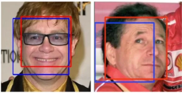
Figure 2.2: Calibrated bounding boxes are better aligned to the faces: the blue rectangles are the most confident detection bounding boxes of 12-net; the red rectangles are the adjusted bounding boxes with the 12-calibration-net. [2].
As shown in the pipeline in Fig. 2.1, the CNN cascade consists of 3 binary classification nets for face detection, while 3 nets serve as calibration nets. The main reason for calibration nets to be adopted in the CNN cascade is to handle situations as shown in Fig. 2.2. Without the calibration step, the next CNN in the cascade would have to evaluate more bounding boxes.
2.2.3 Training Process
In the training process, positive training samples are collected from the Anno- tated Facial Landmarks in the Wild (AFLW) [23] database, which contains about 25k annotated faces in real-world images, where most of them are color images.
Negative training samples are obtained from normal background images not con- taining faces. The caffe [24] library is used for training and testing of the CNN cascade.
10
2.3 Fully Convolutional Networks
2.3.1 Introduction
The main difference between convolutional layers and fully-connected layers inside a CNN, is that convolutional layers are only connected to a region of the input feature map and the parameters are shared across computing on different regions, but both kind of layers basically perform the same dot product operations.
Therefore, any fully-connected layer can be converted to a convolutional layer, provided the filter size is the same as the input feature map with stride size of 1, and the number of filters would be the depth or length of the original fully- connected layer.
2.3.2 Example
Figure 2.3: The architecture of AlexNet [3].
Take the classic CNN model AlexNet [3] as shown in Fig. 2.3 for example, and if converting the first fully-connected layer to a convolutional layer was desired.
The feature map of the original last convolutional layer after pooling is of size [7⇥
7 ⇥ 256], and the original fully-connected layer is of length 4096, which would mean that after conversion, the resulting converted fully-connected layer would be a convolution layer with 4096 filters of size [7 ⇥7⇥256], resulting in a feature map of size [1 ⇥ 1 ⇥ 4096].
11 Similarly, the following fully-connected layer could be converted to a convo- lution layer with 4096 filters of size [1 ⇥ 1 ⇥ 4096], and the last layer could also be converted to a convolution layer with 1000 filters of size [1 ⇥1⇥4096], giving the exactly same results as before.
2.3.3 Applications
Figure 2.4: The efficiency of CNNs for detection [4].
The conversions are extremely useful in practice. As shown in Fig. 2.4, before conversion, the input size was fixed to [14 ⇥ 14], so in order to apply a detector with receptive field of size [14 ⇥14] on an input image of size [16⇥16], applying a sliding window technique would be required. Doing so would involve a large amount of recomputation of the same region; by converting the fully-connected (classifier) layers to convolutional layers, a [2 ⇥ 2] heat map can be achieved by forwarding just once through the model, increasing only the yellow region of com- putation comparing to forwarding an image of size [14 ⇥ 14].
Another example is given in Fig. 2.5. In this case, forwarding an image of size [384 ⇥ 384] would give an input feature map at the last pooling layer of size [12⇥12⇥256], since 384/32 = 12. After feedforwarding the feature map through the last few classifiers, a heat map of size [6 ⇥ 6 ⇥ 1000] is acquired, each entry representing the probability of the corresponding [224 ⇥ 224] crop belonging to
12
Figure 2.5: Results of feedforwarding an image through the fully convolutional version of AlexNet [5].
that class.
In summary, feedforwarding the [384 ⇥ 384] image once through the fully convolutional network gives the same results as passing crops of size [224 ⇥ 224]
with stride size of 32 pixels in a sliding window fashion. The classification results in Fig. 2.5 include various cats, where 282 = tiger cat, 281 = tabby, 283 = persian, and foxes and other mammals.
2.4 Fully Convolutional Network Version of CNN Cascade
2.4.1 Architecture
Suppose there is an image where the original image dimension is [330⇥450⇥
3], and minimum face to find is [48 ⇥ 48] pixels. Since the minimum face to find is [48 ⇥ 48] pixels, and 12-net takes blocks of size [12 ⇥ 12], the image is first downscaled by [4 ⇥ 4], such that each [12 ⇥ 12] block in the downscaled image
13
Figure 2.6: Downscaling of an example image.
corresponds to a [48 ⇥ 48] block in the original image, as shown in Fig. 2.6.
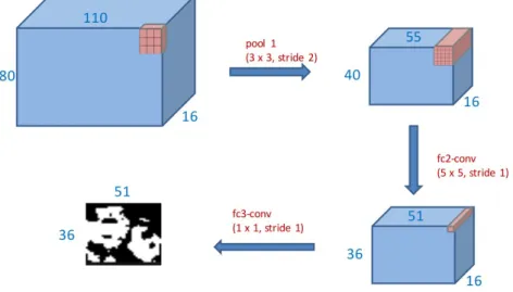
Figure 2.7: Results of feedforwarding an image through the fully convolutional version of 12-net in the CNN cascade architecture.
The fully convolutional version of 12-net is then applied on the downscaled image, resulting in a heat map of size [36⇥51⇥2], with each block corresponding to a [12 ⇥ 12] block in the downscaled image, as shown in Fig. 2.7.
The above step is iteratively applied on images downscaled until either side of the image is smaller than 12 pixels, as shown in Fig. 2.8. Finally, for blocks in heat map which have confidence higher than a predefined threshold, the corresponding position and scale in the original image is saved to be passed on to the later stages of the CNN cascade.
14
Figure 2.8: Images are iteratively downscaled until either side of the image is smaller than 12 pixels.
2.4.2 Computation Reduction
By adopting the fully convolutional version of 12-net, a huge number of com- putation is saved through reduction of the number of convolutional operations.
The total number of multiply-accumulate operations (MACs) using the original sliding window solution and using the modified fully convolutional model can be calculated as follows.
Number o f MACs using sliding window solution
= (#o f sliding window blocks) ⇥ (conv layer MACs + f c layer 1 MACs + f c layer 2 MACs)
= 51 ⇥ 36 ⇥ (10 ⇥ 10 ⇥ 16 ⇥ 3 ⇥ 32+16 ⇥ 5 ⇥ 5 ⇥ 16 + 2 ⇥ 16)
= 91124352 (2.1)
Number o f MACs using f ully convolutional model
= conv layer MACs + f c layer 1 MACs + f c layer 2 MACs
= 110 ⇥ 80 ⇥ 16 ⇥ 3 ⇥ 32+51 ⇥ 36 ⇥ 16 ⇥ 16 ⇥ 52+51 ⇥ 36 ⇥ 2 ⇥ 16
= 15610752 (2.2)
Through calculating the ratio of Equation 2.2 and Equation 2.1, the total num- ber of MACs in 12-net reduce by a factor of 83%.
15
2.5 Summary
In this chapter, it is shown that through modifying the original CNN cascade to a fully convolutional network, a large portion of MACs can be saved, lowering the amount of computation required.
16
Chapter 3 Quantizing
3.1 Introduction
To deploy CNNs onto hardware, an issue we must solve is the storage size of parameters. Even in a relatively small CNN model like the CNN cascade for face detection, which has a total number of 3.98 million parameters, storing such parameters as 32-bit floating-point numbers would require roughly 15.92MB of memory storage. Methods to overcome this problem would be to either decrease the number of parameters, or quantize the parameters to lower precision, while the latter approach is adopted in this work.
As noted in [25], with the help of parameter quantization, the word-length of parameters can be reduced from 32-bits to 2-bits (to represent -1, 0, +1), and the multiply-and-accumulate (MAC) computations for the convolution can be further simplified to 3 to 1 multiplexer operations, as shown in Fig. 3.1. There is 99% cell area reduction between the two arithmetic, as shown in Table. 3.1.
17
18
+
X1
Y W1
X2 W2
X3 W3
+ -0 0 X
Figure 3.1: A quantized neural networks with multiplexers, where the quantized parameters w can only be -1, 0, or +1.
Table 3.1: Cell area comparison of a 32-bit floating point multiplier and a 10-bit 3 to 1 multiplexer.
Arithmetic unit Cell area (µm2) 32-bits floating point multiplier 30344
10-bits 3 to 1 multiplexer 307
Several ways to quantize the parameters from floating-point to fixed-point rep- resentation include:
1. Hard Quantizing :
By observing the range of parameters, according to the number of bits, the range of bits for the integer part and the fractional numbers are assigned, and each parameter is rounded to the closest bin.
2. Quantizing with Stochastic Rounding [26] :
The probability of rounding a parameter to its neighboring bin is propor- tional to the distance to the bins.
3. Modifying the Cost Function [25] :
A penalty is added to the cost function accounting for the distance from predefined bins, quantizing happens during training.
19 4. Network Retraining [6] :
After high precision precision parameters are obtained from normal train- ing, the network is retrained by iteratively quantizing the parameters.
The next sections will describe how these methods work in detail, and the re- sults of applying such techniques on the Face Detection Data Set and Benchmark (FDDB)[22].
3.2 Hard Quantizing
Hard quantizing is quite straightforward, it rounds the parameters to the near- est bin. Given a fixed-point representation as (A,B) , where A is the word-length of the integer part, and B is the word-length of the fractional part, we define e = 2 B, and the range that can be represented would be [ 2A 1,2A 1 2 B].
Given a number x in the representable range, and by defining bxc as the largest number that is a multiple ofe and smaller than or equal to x, the hard quantizing scheme can be denoted as
Round(x) = 8>
<
>:
bxc if bxc x bxc +e2 bxc + e if bxc +2e <x bxc + e
. (3.1)
Shown in Fig. 3.2 are the evaluation results of the hard quantized parameters on FDDB using different word-lengths. It can be observed that 6 bits can almost achieve same accuracy compared to original floating-point parameters.
3.3 Stochastic Rounding
Stochastic rounding is a method proposed in [26], the probability of round- ing a parameter to its neighboring bin is proportional to the distance to the bins.
Following the notations above, its quantizing scheme can be written as
20
Figure 3.2: Evaluating hard quantized parameters on FDDB
Round(x) = 8>
<
>:
bxc w.p. 1 x bxce bxc + e w.p. x bxce
. (3.2)
The main intuition of stochastic rounding comes from the fact that it is an unbiased rounding scheme, i.e. E(Round(x)) = x.
Shown in Fig. 3.3 are the evaluation results of the stochastically rounded pa- rameters on FDDB using different word-lengths. It can be observed that 5 bits can almost achieve same accuracy compared to original floating-point parame- ters., only at the cost of more false positives. The results of stochastic rounding with word-length of 8 bits even surpasses results obtained from using the original floating-point parameters.
21
Figure 3.3: Evaluating stochastically rounded parameters on FDDB
3.4 Modifying the Cost Function
This quantizing strategy is proposed by [25]. [27] has shown a way to initialize parameters when using tanh as the activation function is
W ⇠ U
" p pnin+6nout,
p6 pnin+nout
#
, (3.3)
where nin and nout are the number of input and output nodes of a particular layer.
To quantize the coefficients into three bins, the centroids of the quantization bins are the tri-section points
Q =
( 2p
6
3pnin+nout,0, 2p 6 3pnin+nout
)
. (3.4)
This method uses a two-step approach composed of soft-quantization and hard-quantization to quantize the parameters. In the soft-quantization stage, the
22
quantization effect is considered as a regularization term in the back-propagation step of neural networks training.
Instead of the original cost function, a regularization term is added to make the parameters concentrate to the centroids of the quantization bins as follows,
J(x) =a|y h(x)|2+ (1 a) wi j qnearest 2, (3.5) where
qnearest =argmin
q2Q wi j q , (3.6)
a 2 [0,1] is used to control the weights of error cost and quantization cost. Ini- tially, a is equal to 1, placing more priority on the correctness of classification result, anda decays with a step Da as more training epochs go by, which means the importance of quantization cost grows.
After soft-quantization, hard-quantization is then applied to decide the final model parameters as follows.
wi j = 8>
>>
><
>>
>>
:
+1 if x 3pnp6
j+nj+1
1 if x 3pnp6
j+nj+1
0 else
(3.7)
3.5 Network Retraining
A quantizing method was proposed in [6] through retraining a normal high precision pretrained network, by following an iterative process as shown in Fig. 3.4.
In each iterative step, the original parameters are first quantized. Next, the quan- tized parameters are feedforwarded, and the output error is calculated. At last, the error gradients are calculated, but used for updating the high precision weights.
The high precision weights are then quantized, and the whole process starts over again.
The validation accuracy of the retrained models are shown as follows:
23
Figure 3.4: Network retraining proposed in [6]
• 12-net
2-bit validation accuracy: 0.915
• 24-net
2-bit validation accuracy: 0.982
• 48-net
2-bit validation accuracy: 0.987
• 12-calibration-net
5-bit validation accuracy: 0.188
• 24-calibration-net
5-bit validation accuracy: 0.246
• 48-calibration-net
2-bit validation accuracy: 0.316 It was not successful training 12-calibration-net and 24-calibration-net using word-length of 5 bits, but it can observed that removing these two calibration nets does not decrease too much accuracy on the FDDB [22], as shown in Fig. 3.5.
3.6 Summary
In this chapter, several different schemes for quantizing are compared and evaluated on the FDDB, and the applied method can reduce the storage size for the parameters from 32-bits to 2-bits.
24
Figure 3.5: Evaluating retrained parameters on FDDB
Chapter 4
Hardware Implementation
4.1 Introduction
This chapter describes the exploration of the design space for implementing a CNN accelerator on a Xilinx XC7020 FPGA board. We quantitatively analyze the computing throughput and required bandwidth using the roofline model[7], an analytical design scheme, to find the solution with best performance and lowest FPGA resource requirement. The benefits of quantizing towards computational ability of the final design is also demonstrated.
4.2 Potential Accelerations of a Typical CNN
Figure 4.1: Graph of a convolutional layer [7].
25
26
A CNN convolutional layer is shown in Fig. 4.1. It has been shown in [28]
that 90% of computation in CNN models come from convolutional operations during the feedforward process. Therefore, work in this thesis will be focused on accelerating the convolutional layer.
A straightforward pseudo code of a convolutional layer can be written as
f o r ( row = 0; row < R; row++)
f o r ( c o l = 0; c o l < C; c o l ++)
f o r ( to = 0; to <M; to ++)
f o r ( t i = 0; t i < N; t i ++) f o r ( i = 0; i < K ; i ++)
f o r ( j = 0; j < K ; j ++) output fm [ to ] [ row ] [ c o l ] +=
weights [ to ] [ t i ] [ i ] [ j ] ⇤
i n p u t f m [ t i ] [ S ⇤ row + i ] [ S ⇤ c o l + j ] ;
where R and C are respectively the number of rows and columns in the output feature map, M and N are the number of channels in the input and output feature map, and K and S are the dimension and stride of the filters.
4.3 The Roofline Model
Figure 4.2: The roofline model [8].
27 A few aspects that should be noticed when designing hardware include compu- tation, communication (retrieving and storing data from DRAMs) and bandwidth.
The roofline model is proposed in [8] to address such problems. Floating-point performance (GFLOPS) is often used to measure throughput of hardware, and the maximum attainable performance is upper bounded by the peak performance provided by the hardware platform, while the actual performance is related to the computation to communication (CTC) ratio
Attainable Per f ormance = min 8>
<
>:
Computational Roo f CTC Ratio ⇥ BW
, (4.1)
where BW is the bandwidth provided by the hardware platform.
As shown in Fig. 4.2, using the same hardware platform, Algorithm 2 achieves higher performance because it utilizes better data reuse, while Algorithm 1 per- forms worse resulting from not effectively communicating with off-chip memory.
4.4 Loop Tiling
With such large amount of input feature maps, weight and bias parameters, it is not feasible to store all data in on-chip memory. Thus, loop tiling is a must for the CNN accelerator to be implemented. The tiled version of a convolutional layer is shown in the following pseudo code.
f o r ( row = 0; row < R; row += T r )
f o r ( c o l = 0; c o l < C; c o l += T c )
f o r ( to = 0; to <M; to += T m )
f o r ( t i = 0; t i < N; t i += T n ) {
/ / load f e a t u r e maps and weights
/ / on chip computation t h a t can be f u r t h e r optimized f o r ( t r r = row ; t r r < min ( row + T r , R ) ; t r r ++)
f o r ( t c c = c o l ; t c c < min ( c o l + T c , C ) ; t c c ++)
28
f o r ( too = to ; too < min ( to + T m , M) ; too ++)
f o r ( t i i = t i ; t i i < min ( t i + T n , N ) ; t i i ++) f o r ( i = 0; i < K ; i ++)
f o r ( j = 0; j < K ; j ++)
output fm [ too ] [ t r r ] [ t c c ] +=
weights [ too ] [ t i i ] [ i ] [ j ] ⇤
i n p u t f m [ t i i ] [ S ⇤ t r r + i ] [ S ⇤ t c c + j ] ; }
Loop iterators i and j are not tiled, since the kernel dimension size K is usually a small number. Different tiling sizes could lead to very different computation performance, and the choice of such parameters will be discussed in the following section.
4.5 Computation Optimization
4.5.1 Loop Unrolling
From standard polyhedral-based data dependence analysis [29], the data shar- ing relations between different loop iterations of a loop dimension can be catego- rized as follows:
• Irrelevant : loop iterator does not appear in any access functions of an array
• Independent : data space accessed on an array is totally separable along a certain loop dimension
• Dependent : data space accessed on an array is not separable along a certain loop dimension
The data sharing relations of the pseudo code above is shown in Fig. 4.3. Since too and tii are not dependent on any of the arrays, they can be unrolled without
29
Figure 4.3: The data sharing relations [8].
creating complex hardware connections. The final pseudo code of the accelerator structure is shown below.
f o r ( row = 0; row < R; row += T r )
f o r ( c o l = 0; c o l < C; c o l += T c )
f o r ( to = 0; to <M; to += T m )
f o r ( t i = 0; t i < N; t i += T n ) {
/ / load f e a t u r e maps and weights
/ / on chip computation f o r ( i = 0; i < K ; i ++)
f o r ( j = 0; j < K ; j ++)
f o r ( t r r = row ; t r r < min ( row + T r , R ) ; t r r ++) f o r ( t c c = c o l ; t c c < min ( c o l + T c , C ) ; t c c ++)
#pragma HLS PIPELINE
f o r ( too = to ; too < min ( to + T m , M) ; too ++)
#pragma HLS UNROLL
f o r ( t i i = t i ; t i i < min ( t i + T n , N ) ; t i i ++)
#pragma HLS UNROLL
output fm [ too ] [ t r r ] [ t c c ] +=
weights [ too ] [ t i i ] [ i ] [ j ] ⇤
i n p u t f m [ t i i ] [ S ⇤ t r r + i ] [ S ⇤ t c c + j ] ; }
30
4.5.2 Tile Size Selection
As mentioned before, the size of tiling plays an important role on the final performance of the generated hardware. The space of all legal tile sizes is as shown in Equation 4.2.
8>
>>
>>
>>
>>
>>
><
>>
>>
>>
>>
>>
>>
:
0 < Tm⇥ Tn (number o f processing elements) 0 < Tm M
0 < Tn N 0 < Tr R 0 < Tc C
(4.2)
Given the tile sizes, the computational roof can then be calculated as
computational roo f
= total number o f operations number o f execution cycles
= 2 ⇥ R ⇥C ⇥ M ⇥ N ⇥ K ⇥ K
dTMme ⇥ dTNne ⇥TRr⇥TCc⇥ (Tr⇥ Tc⇥ K ⇥ K + P)
⇡ 2 ⇥ R ⇥C ⇥ M ⇥ N ⇥ K ⇥ K
dTMme ⇥ dTNne ⇥ R ⇥C ⇥ K ⇥ K, (4.3) where P is the pipeline depth 1.
4.6 CTC Ratio and Benefits from Quantizing
Another important design factor to consider is the computation to communica- tion (CTC) ratio, as it usually decides the final attainable performance. It denotes the number of operations performed for each memory access, indicating the level of data reuse. As shown in [8], the CTC Ratio of the final hardware structure can be calculated in Equation 4.12, whereain,awght,aout and Bin, Bwght, Bout are respectively the trip counts and buffer sizes of memory accesses.
31
CTC Ratio
= total number o f operations total amount o f exeternal data access
= 2 ⇥ R ⇥C ⇥ M ⇥ N ⇥ K ⇥ K
ain⇥ Bin+awght⇥ Bwght+aout⇥ Bout (4.4)
where
ain=awght= M Tm⇥ N
Tn⇥ R Tr ⇥C
Tc (4.5)
aout= M Tm⇥ R
Tr ⇥C
Tc (4.6)
Bin=Tn(STr+K S)(STc+K S) (4.7)
Bwght=TmTnK2 (4.8)
Bout=TmTrTc (4.9)
0 <Bin+Bwght+Bout BRAMcapacity (4.10) (4.11)
Because of applying quantizing to the weight and bias parameters from 32- bit floating-point to 2-bit fixed-point numbers as mentioned in Chapter 3, we can gain some advantages in the CTC ratio. Since the parameters are 2-bit fixed-point numbers and the layer with most parameters in the CNN cascade architecture is the second convolution layer of net-48, with 64 filters of size 64 ⇥ 5 ⇥ 5, totaling 102400 parameters, which is equal to merely 25KB memory storage, the parame- ters of any single layer can easily be stored in the on-chip BRAM of the hardware platform. This results inawght to decrease to 1, and Bwght to remain unchanged or vary slightly, which can in turn increase the CTC ratio, possibly leading to better attainable performance. The resulting CTC ratio after such optimization can then be calculated as
32
CTC Ratio
= total number o f operations total amount o f external data access
= 2 ⇥ R ⇥C ⇥ M ⇥ N ⇥ K ⇥ K
ain⇥ Bin+Bwght+aout⇥ Bout (4.12)
4.7 Optimal Parameters
Table 4.1: Maximum execution cycles under different tile sizes Pipeline (Tm,Tn) Max. Execution Cycles
no (1, 1) 134113995
yes (1, 1) 81967538
yes (4, 4) 19532584
yes (16, 1) 13828235
yes (10, 2) 13244457
yes (16, 8) 8939162
yes (64, 7) 1281051
As seen in previous equations, the CTC ratio and computational roof are highly related to tile size selection. Table 4.1 shows resulting maximum exe- cution cycles under different tile sizes. It can be observed that under the same number of processing elements, the resulting latency can vary greatly. Similar to [8], we enumerate all possible tile sizes to find the optimal solution, and the best configuration through all convolution layers is (Tm,Tn) = (64, 7).
4.8 Block Diagram
The block diagram of the hardware implementation is shown in Fig. 4.4. The Zynq7 processing system is a dual-core Cortex-A9 processor provided on Xilinx
33
Figure 4.4: Block diagram
FPGAs, used for configuring other blocks to start or initiate transfers. It is also responsible for providing parameters to the CNN accelerator, such as the width, height and channels of the input feature map, and the number of weights, etc. The AXI4 Lite bus transfers basic commands, while the AXI4 Stream bus transfers data like the input and output feature maps, and the weight and bias parameters.
An AXI Timer is used for timing the execution of performing operations on either the CNN accelerator or the CPU, and the UART displays information to the host computer. DMA (Direct Memory Access) engines are FIFO (first in, first out) transmitters that can effectively transfer data from the DDR3 memory to the CNN accelerator, or the other way around.
4.9 Computation Engine
Unrolling of the bottom loops as mentioned in Section 4.5.1 generates a tree- shaped poly structure as shown in Fig. 4.5. In the case of (Tm,Tn) = (64, 7), the resulting hardware would have 7 inputs from input feature maps, 7 inputs from
34
Figure 4.5: Computation Engine [8]
weights and one input from bias. 64 instances of the same structure would then be duplicated to resemble the tile size Tm=64.
4.10 Experiments
Implementation of the hardware is done by using Vivado HLS, a high level synthesis tool from Xilinx, that can generate Verilog and VHDL RTL scripts from C or C++ code. An IP core can then be exported to be used in the Vivado tool, and other built-in IP blocks such as DMA (Direct Memory Access) engines and AXI timers can be added to interact with the user-defined IP core. The whole design can then be synthesized, written to a bitstream, and programmed on the target FPGA. The user can then choose to test the hardware through installing an operating system on the board, or by simply using a bare-metal solution in the environment of Xilinx SDK (Software Development Kit).
4.10.1 Development Device
The experiments were carried out on a Xilinx XC7020 FPGA board. Due to limited resources, several tile sizes utilizing more processing elements (DSPs) do
35 not fit under such constraints. However, the synthesis reports provided by Vivado HLS give moderately precise latency (number of execution cycles) information.
Therefore, we derive the expected time and corresponding performance (GFLOPS) by computing the ratio of execution cycles as shown in Table 4.2. Although the final (Tm,Tn) = (64, 7) design does not fit on the XC7020 board, according to Fig. 4.6 provided by Xilinx, it is deployable on the XC7Z100 board.
Table 4.2: Performance (GFLOPS) on the second convolutional layer of 48-net under different tile sizes.
(Tm, Tn) Max. Cycles BRAM (%) DSP (%) FF (%) LUT (%) Time (ms) GFLOPS
(1, 1) 6885145 13 15 3 12 131.4 1.51
(4, 4) 1628054 14 75 7 22 32.2 6.15
(16, 1) 1148639 14 85 12 36 22.1 8.97
(16, 8) 773952 14 375 30 74 14.8 13.42
(64, 7) 116582 13 901 106 253 2.22 89.30
Figure 4.6: Resources of different Zynq devices [9].
36
4.10.2 Performance Comparison to CPU
Table 4.3: Performance comparison to CPU
CPU FPGA
time (ms) time (ms) GFLOPS
12-net conv1 381 0.32 47.52
12-net fc2-conv 1059 0.62 75.81
12-net fc3-conv 5 0.007 33.57
24-net conv1 167 0.14 54.86
48-net conv1 811 0.67 55.48
48-net conv2 2787 2.22 89.30
Total time (ms) 5210 3.98
Avg. GFLOPS 0.06 76.8
Shown in Table 4.3 is the performance comparison between the implemented accelerator and a software based solution running on the dual-core Cortex-A9 processor of the FPGA. As observed, an average performance of 76.8 GFLOPS is achieved, accelerating the software based solution by up to 1000 times. The ad- ditional performance compared to 61.62 GFLOPS achieved in [7] mainly comes from caching the weight and bias parameters on chip, instead of loading parame- ters each time during computation.
4.11 Summary
In this chapter, the exploration of the design space for implementing the CNN accelerator on a Xilinx XC7020 FPGA board is described. The computing through- put and required bandwidth is quantitatively analyzed using the roofline model[7], to find the solution with best performance and lowest FPGA resource requirement.
The benefits of quantizing towards computational ability of the final design is also demonstrated through experiments and synthesis reports from Vivado HLS.
Chapter 5 Conclusion
In this thesis, several techniques were proposed to bridge the gap between a deep learning model for face detection and implementing it on VLSI or FPGA platforms.
In Chapter 2, it was shown that through modifying the original CNN cascade for face detection to a fully convolutional network, 83% of multiply-accumulate operations (MACs) can be saved, decreasing the amount of computation. Differ- ent quantizing methods were discussed and compared through experiments carried out on the Face Detection Data Set and Benchmark (FDDB)[22] in Chapter 3, and it was shown that through applying a quantizing technique, the word-length of parameters could reduce from 32-bits to 2-bits while not affecting much perfor- mance. Finally in Chapter 4, the exploration of the design space for implementing the architecture on a Xilinx XC7020 FPGA board was discussed, and benefit- ing from quantizing, an increase in computational ability was also demonstrated, achieving a performance of 76.8 GFLOPS.
With the proposed optimizations, the difficulties of deploying CNN models on mobile or embedded systems under power constraints should be greatly decreased, accelerating speed compared to CPU-based solutions.
37
38
Reference
[1] S. S. Farfade, M. J. Saberian, and L.-J. Li, “Multi-view face detection us- ing deep convolutional neural networks,” in Proceedings of the 5th ACM on International Conference on Multimedia Retrieval (ICMR ’15), 2015, pp.
643–650.
[2] H. Li, Z. Lin, X. Shen, J. Brandt, and G. Hua, “A convolutional neural net- work cascade for face detection,” in Proc. IEEE Conference on Computer Vision and Pattern Recognition (CVPR), June 2015, pp. 5325–5334.
[3] A. Krizhevsky, I. Sutskever, and G. E. Hinton, “Imagenet classification with deep convolutional neural networks,” in Proc. in Neural Information Pro- cessing Systems (NIPS 2012), 2012, p. 4.
[4] P. Sermanet, D. Eigen, X. Zhang, M. Mathieu, R. Fergus, and Y. LeCun,
“Overfeat: Integrated recognition, localization and detection using convolu- tional networks,” in Proc. International Conference on Learning Represen- tations (ICLR2014). CBLS, April 2014.
[5] “Net surgery,” https://github.com/BVLC/caffe/blob/master/examples/net surgery.ipynb, 2015, [Online].
[6] S. Anwar, K. Hwang, and W. Sung, “Fixed point optimization of deep con- volutional neural networks for object recognition,” in Proc. IEEE Interna- tional Conference on Acoustics, Speech and Signal Processing (ICASSP), April 2015, pp. 1131–1135.
39
40
[7] C. Zhang, P. Li, G. Sun, Y. Guan, B. Xiao, and J. Cong, “Optimizing fpga-based accelerator design for deep convolutional neural networks,” in Proc. 23rd International Symposium on Field-Programmable Gate Arrays (FPGA), 2015.
[8] S. Williams, A. Waterman, and D. Patterson, “Roofline: an insightful vi- sual performance model for multicore architectures,” Communications of the ACM, vol. 52, pp. 65–76, April 2009.
[9] Xilinx, “Zynq-7000 all programmable soc overview (ds190 v1.9),” Tech.
Rep., January 2016.
[10] P. Viola and M. J. Jones, “Robust real-time face detection,” International Journal of Computer Vision, vol. 57, pp. 137–154, May 2004.
[11] B. Froba and A. Ernst, “Face detection with the modified census transform,”
in Proceedings. Sixth IEEE International Conference on Automatic Face and Gesture Recognition, May 2004, pp. 91–96.
[12] H. Jin, Q. Liu, H. Lu, and X. Tong, “Face detection using improved lbp under bayesian framework,” in Proc. Third International Conference on Image and Graphics (ICIG), vol. 57, December 2004, pp. 306–309.
[13] L. Zhang, R. Chu, S. Xiang, S. Liao, and S. Z. Li, “Face detection based on multi-block lbp representation,” in Proceedings of the 2007 international conference on Advances in Biometrics (ICB), August 2007, pp. 11–18.
[14] S. Yan, S. Shan, X. Chen, and W. Gao, “Locally assembled binary (lab) feature with feature-centric cascade for fast and accurate face detection,”
in Proc. IEEE Conference on Computer Vision and Pattern Recognition (CVPR), June 2008, pp. 1–7.
41 [15] X. Wang, T. X. Han, and S. Yan, “An hog-lbp human detector with partial occlusion handling,” in Proc. IEEE 12th International Conference on Com- puter Vision, September 2009, pp. 32–39.
[16] T. Mita, T. Kaneko, and O. Hori, “Joint haar-like features for face detection,”
in Proc. Tenth IEEE International Conference on Computer Vision (ICCV), vol. 2, October 2005, pp. 1619–1626.
[17] K. He, X. Zhang, S. Ren, and J. Sun, “Delving deep into rectifiers: Sur- passing human-level performance on imagenet classification,” CoRR, vol.
abs/1502.01852, 2015.
[18] A. Karpathy and F. Li, “Deep visual-semantic alignments for generating im- age descriptions,” CoRR, vol. abs/1412.2306, 2014.
[19] N. Jaitly, V. Vanhoucke, and G. E. Hinton, “Autoregressive product of multi- frame predictions can improve the accuracy of hybrid models,” in Proc.
INTERSPEECH 2014, 15th Annual Conference of the International Speech Communication Association, Singapore, September 14-18, 2014, 2014, pp.
1905–1909.
[20] X. Zhang and Y. LeCun, “Text understanding from scratch,” CoRR, vol.
abs/1502.01710, 2015.
[21] M. Denil, B. Shakibi, L. Dinh, M. Ranzato, and N. de Freitas, “Predicting parameters in deep learning,” CoRR, vol. abs/1306.0543, 2013.
[22] V. Jain and E. Learned-Miller, “Fddb: A benchmark for face detection in unconstrained settings,” University of Massachusetts, Amherst, Tech. Rep.
UM-CS-2010-009, 2010.
[23] M. Kstinger, P. Wohlhart, P. M. Roth, and H. Bischof, “Annotated facial landmarks in the wild: A large-scale, real-world database for facial landmark
42
localization,” in Proc. IEEE International Conference on Computer Vision Workshops (ICCV Workshops), October 2011, pp. 2144–2151.
[24] Y. Jia, E. Shelhamer, J. Donahue, S. Karayev, J. Long, R. Girshick, S. Guadarrama, and T. Darrell, “Caffe: Convolutional architecture for fast feature embedding,” arXiv preprint arXiv:1408.5093, 2014.
[25] P.-H. Hung and S.-Y. Chien, “Deep neural networks on video sensor net- works: Quantized and distributed approaches,” Master’s thesis, National Tai- wan University, June 2015.
[26] S. Gupta, A. Agrawal, K. Gopalakrishnan, and P. Narayanan, “Deep learning with limited numerical precision,” in Proceedings of the 32nd International Conference on Machine Learning (ICML), 2015, pp. 1737–1746.
[27] Y. Bengio and X. Glorot, “Understanding the difficulty of training deep feed- forward neural networks,” in Proceedings of AISTATS 2010, vol. 9, May 2010, pp. 249–256.
[28] J. Cong and B. Xiao, “Minimizing computation in convolutional neural net- works,” Artificial Neural Networks and Machine Learning (ICANN), pp.
281–290, 2014.
[29] L.-N. Pouchet, P. Zhang, P. Sadayappan, and J. Cong, “Polyhedral-based data reuse optimization for configurable computing,” in Proceedings of the ACM/SIGDA international symposium on Field programmable gate arrays (FPGA), 2013, pp. 29–38.
![Figure 2.1: Testing pipeline from [2].](https://thumb-ap.123doks.com/thumbv2/9libinfo/9608850.634328/26.892.146.869.429.562/figure-testing-pipeline-from.webp)
![Figure 2.3: The architecture of AlexNet [3].](https://thumb-ap.123doks.com/thumbv2/9libinfo/9608850.634328/28.892.149.735.602.787/figure-the-architecture-of-alexnet.webp)
![Figure 2.4: The efficiency of CNNs for detection [4].](https://thumb-ap.123doks.com/thumbv2/9libinfo/9608850.634328/29.892.242.628.351.591/figure-efficiency-cnns-detection.webp)
![Figure 2.5: Results of feedforwarding an image through the fully convolutional version of AlexNet [5].](https://thumb-ap.123doks.com/thumbv2/9libinfo/9608850.634328/30.892.265.603.147.442/figure-results-feedforwarding-image-fully-convolutional-version-alexnet.webp)