平衡渦旋模型之熱與動量動力效率

(1)

國立臺灣大學理學院大氣科學系碩士論文

Department of Atmospheric Science College Science

National Taiwan University Master Thesis

平衡渦旋模型之熱與動量動力效率

Dynamic Efficiency of Heat and Momentum in Balanced Vortex Model

許天耀 Tien-Yiao Hsu

指導教授：郭鴻基博士 Advisor: Hung-Chi Kuo, Ph.D.

中華民國 104 年 7 月

July, 2015

(2)

誌謝

一篇作品的完成不只需要個人努力，亦需有旅途中各方貴人的相助。

感謝郭老師給予的指導，討論，支持與肯定。這是我前進的動力。

美雲超過兩年的關懷與照顧，無法用三言兩語表達，除了感謝還是感謝。維毅，虹叡，郁涵，徐驊，世顥，佑宇，政友，王珩，立中，佳瑩，映如等人給予的協助點滴在心。這是一間溫暖且包容的實驗室，

有緣於此停泊，甚感幸運。緣分的推演人無可知，而我感謝這些安排。

我要感謝家人與韋龍，在這些日子裏承擔我的任性。

最後，我要感謝自己，完成當初的承諾。這些日子裡，你更認識了自己，接受自己的缺點，也知道自己可以成為甚麼樣的人――你比過去更有能力參與自己的人生，謝謝你。

寫下這些文字的同時，窗外蟬聲唧唧，正如同兩年前的今天一樣，

瀰漫著慵懶與未知。不同的是我即將完成學業離開此處。走入未來，

如同走入森林，失去方向，充滿恐怖與不安，卻帶點雀躍和悸動。何處存在美麗的瀑布與甘泉？尋得之時必然知曉，因吾等已然品嘗。

2015/06/25 天耀於一片唧唧蟬聲

(3)

摘要

觀測資料顯示眼牆置換 (ERC) 過程會產生不同的結果。Kuo et al. (2009) 發現在置換過程結束後，大約 28% 的颱風會繼續增強。Yang et al. (2013) 針對雙眼牆置換完成後的演化，發展出四個分類。他們指出不同分類的颱風在強度的演化上有明顯的不同，於 T-V 圖中亦具有不同的演化路徑。

Hack and Schubert (1986) 提出熱動力效率 η (r, z, t) 之概念。此物理 量能夠定量描述總位能 (P) 轉換到總動能 (P) 之能量轉換速率 (C)，並 以加熱 (Q) 最為量度基準。該文獻指出儘管總加熱量 (H) 維持一樣，

不同的渦漩結構會產生極為不同的轉換效率。在此研究中，我們將利用熱動力效率，來測試單雙眼牆颱風 Francis (2004) 之轉換效率反應。

我們發現外眼牆在動力上能夠透過減少羅士比長度而提高渦漩的能量轉換效率達 50% 至 400%，而改變內外眼牆之加熱率比重 (從 1 : 2 至 2 : 1) 則可以強化能量轉換效率達 100% 至 600%。

除了此研究主要使用的圓柱座標外，本論文也推導在準地轉理論 (卡式座標)，卡式座標，球座標與淺水模型之動力效率，可供參考與應用於其他尺度平衡動力研究之用。

關鍵字：平衡渦漩、熱動力效率、動量動力效率、雙眼牆、次環流

(4)

ABSTRACT

The observation data shows that the eyewall replacement cycle (ERC) results in different consequences. Kuo et al. (2009) found that approximately 28% of typhoons strengthen after the formation of secondary eyewall. Yang et al. (2013) developed four categories to classify the situations after the formation. They found these four categories exhibit different behaviors on in- tensity and routes on T-V diagram.

“Dynamic efficiency of heat” η (r, z, t)) developed by Hack and Schu- bert (1986) is to examine the effect of heating on the energy conversion rate (C) converting total potential energy (P) into total kinetic energy (K) They also pointed out that efficiencies vary under different vortex structures while total heating remains the same. In this study, we would apply dynamic efficiencies to examine the response of concentric eyewall cyclone Francis (2004).

We find that the presence of outer eyewall enhances the efficiency response by approximately 50% to 400% through reducing Rossby length (λR) while changing the heating ratio between inner and outer eyewalls from 1 : 2 to 2 : 1 enhances the efficiency by 100% to 600% (total heating is fixed).

Apart from cylindrical coordinates, we also derive the dynamic efficiencies in quasi-geostrophic theory (Cartesian coordinates), Cartesian coordinates, spherical coordinates, and shallow water model for potentially application to other balance dynamics in different scales.

(5)

Keywords: balanced vortex, dynamic efficiency of heat, dynamic efficiency of momentum, concentric eyewall, double eyewall, secondary circulation

(6)

LIST OF FIGURES

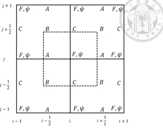
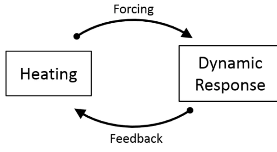
1 Finite-difference grid for solutions of (3.1) . . . 33 2 General scheme of a tropical cyclone system. Heating is treated as a forc-

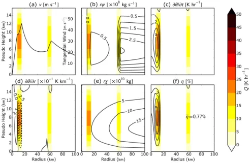
ing to generate dynamic response which feedbacks to heating at the same time. Our work is to diagnose the effect of the heating and to discuss its dynamic response. . . 34 3 The flowchart of a two-regioned barotropic model which represents a sin-

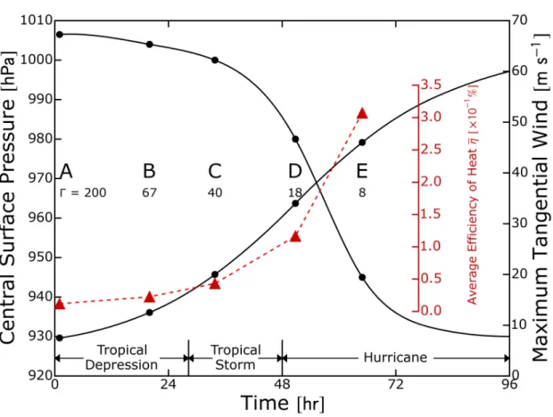
gle eyewall tropical cyclone. (a) Tangential wind profile (m s⁻¹). (b) In- duced streamfunction rψ (×10¹³ kg day⁻¹). (c) Local heating rate ∂T /∂t (K day⁻¹). (d) ∂T /∂r (×10⁻³ K km⁻¹). Time interval is one hour. (e) Corresponding solution rχ (×10¹⁰ kg). (f) Dynamic efficiency of heat (%). Shades in all graphs are adiabatic heating (K day⁻¹). The model setting is adapted from Schubert and Hack (1982) and is listed in table 2 (case D). . . 39 4 Evolution with repect to total time (hr) of average efficiency of heat η

(×10⁻¹%, red line), maximum wind speed (m s⁻¹), Γ = √

A/C (labeled under each stage) and central pressure (hpa) of five stages during a typical tropical cyclone development. Time interval is one hour. The model settings are adapted from Schubert and Hack (1982) and are listed in table 2. 40

(9)

5 Isolines of total heat response (∫_b₂

0

∂T

∂trdr/∫_b₂

0 Qrdr, black line) and aver- age efficiency η (%, red line) in terms of core size a (km) and core rotation strength (ˆµ− µ) /µ with different heating region b2 = a± 50km. A, B, C, D and E represent five stages of typical tropical cyclone. The model settings are the same as Fig. 4 . . . 41 6 The flowchart of a five-regioned barotropic model which represents a dou-

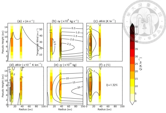
ble eyewall tropical cyclone. (a) Tangential wind profile (m s⁻¹). (b) In- duced streamfunction rψ (×10⁸ kg s⁻¹). (c) Local heating rate ∂T /∂t (K hr⁻¹). (d) ∂T /∂r (×10⁻¹ K km⁻¹). Time interval is one hour. (e) Corresponding solution rχ (×10¹⁰ kg). (f) Dynamic efficiency of heat (%). Shades in all graphs are adiabatic heating (K day⁻¹). The model setting is adapted from Rozoff et al. (2008) and listed in table 4 (case A_dyn+ A_heat). . . 42 7 The flowchart of a five-regioned barotropic model which represents a dou-

ble eyewall tropical cyclone. (a) Tangential wind profile (m s⁻¹). (b) In- duced streamfunction rψ (×10⁸ kg s⁻¹). (c) Local heating rate ∂T /∂t (K hr⁻¹). (d) ∂T /∂r (×10⁻¹ K km⁻¹). Time interval is one hour. (e) Corresponding solution rχ (×10¹⁰ kg). (f) Dynamic efficiency of heat (%). Shades in all graphs are adiabatic heating (K day⁻¹). The model setting is adapted from Rozoff et al. (2008) and listed in table 4 (case B_dyn+ B_heat). . . 42 8 The flowchart of a five-regioned barotropic model which represents a dou-

ble eyewall tropical cyclone. (a) Tangential wind profile (m s⁻¹). (b) In- duced streamfunction rψ (×10⁸ kg s⁻¹). (c) Local heating rate ∂T /∂t (K hr⁻¹). (d) ∂T /∂r (×10⁻¹ K km⁻¹). Time interval is one hour. (e) Corresponding solution rχ (×10¹⁰ kg). (f) Dynamic efficiency of heat (%). Shades in all graphs are adiabatic heating (K day⁻¹). The model setting is adapted from Rozoff et al. (2008) and listed in table 4 (case C_dyn+ C_heat). . . 43

(10)

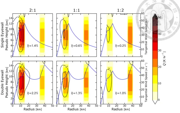
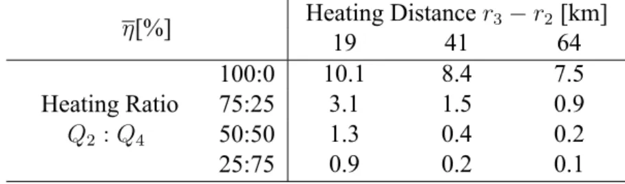
9 Three settings of tangential wind speed profile (m s⁻¹, solid lines) and heat constant ˆQ (K hr⁻¹). The coupled results of average efficiency η (%) are listed in the top-right table. Time interval is one hour. The model settings are adapted from Rozoff et al. (2008) and are listed in table 4. . . 43 10 The wind profile (m s⁻¹, solid line), heating (K hr⁻¹, shading) and result

efficiency η (×10⁻¹%, contour) of six different cases. The wind profiles represent single (A_dyn) and double (C_dyn) eyewall and in the first and second rows, respectively. The heating ratios between inner and outer eyewalls are 2 : 1, 1 : 1 and 1 : 2 (shown in table 4) in the first, second and third columns, respectively. . . 44 11 The wind profile (m s⁻¹, solid line), heating (K hr⁻¹, shading) and result

efficiency η (×10⁻¹%, contour) of six different cases. The wind profiles represent single, double, and larger double eyewall (A_dyn, B_dyn and C_dyn) in the first, second and third columns, respectively. The heating is totally on inner eyewall and outer eyewall (80.9, 29.3 and 18.4 K hr⁻¹) in the first and second rows, respectively. . . 44 12 Four cases to compare hub-cloud profile’s efficiency. The first row is

wind profile, heating (K hr⁻¹, shading), and result efficiency η (×10⁻¹%, contour), the second row shows the induced vertical motion w (m s⁻¹) and local heating rate ∂T /∂t (K hr⁻¹). The model settings are adapted from Schubert et al. (2007) and are listed in table 3 . . . 47 13 Average dynamic efficiency of heat η (%) in various height of maximum

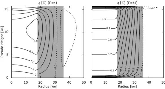
heating z_max(km). Heating thickness is half of the atmosphere height. A, B and C represent wind profile as in Fig. 9 Notice that heating is now totally in the first eyewall. . . 48 14 Distribution of dynamic efficiency of heat (%, contour) under pre-existing

baroclinity (shaded) with different Γ (4 and 64). B = 1× 10⁻⁶s⁻²in both cases. . . 48

(11)

15 Distribution of dynamic efficiency of heat (%, contour) solved under barotropic (upper panel) and baroclinic (lower panel) conditions. . . 49 16 Distribution of dynamic efficiency of heat (%, contour) solved under barotropic

(upper panel) and baroclinic (lower panel) conditions. . . 50 17 Average dynamic efficiency of heat η (%) in terms of relative rotation

strength ˆµ₄/ˆµ₃ and outer eyewall position r₃ (km). Total local heat re- sponse is 12.6% throughout the domain. . . . 51 18 Average dynamic efficiency of heat η (%) in terms of wind shape param-

eter λ_dyn and heating shape parameter λ_Q. Nine thumbnails are drawn in the right. Total local heat response is 12.6% throughout the domain. . . . 52 19 A stable configuration of m and b. The red and blue arrows are buoyancy

restorcing force and inertial restoring force, respectively. . . 70 20 An unstable configuration of m and b. The red and blue arrows are buoy-

ancy restorcing force and inertial restoring force, respectively. . . 70 21 The comparison between cylindrical and spherical coordinates. . . 73

(12)

LIST OF TABLES

1 General form of Eliassen-Sawyer circulation equation in different coordinates . . . 29 2 Two-regioned model settings for typical development of tropical cyclone.

H₀= 10 K day⁻¹ (250km)² . . . 38

3 Three-regioned model settings for u-shaped wind profile. H₀ = 125 K day⁻¹ (50km)² 38 4 Five-regioned model settings for decoupled wind and heating profile. H₀=

125 K day⁻¹ (50km)² . . . 38 5 Average efficiency η (%) with respect to heating distance r3−r2(km) and

heating ratio Q₂ : Q₄ between inner and outer eyewall. . . 46 6 General form of Eliassen-Sawyer circulation equation in cylindrical and

spherical coordinates . . . 76

(13)

(14)

CHAPTER 1

INTRODUCTION

A cyclone intensifies itself by storing the available potential energy through latent of water vapor and releasing it into kinetic energy. Charney and Eliassen (1964) proposed Condi- tion Instability of the Second Kind (CISK) to explain the initiation of the tropical depres- sion. Later, Schubert and Hack (1982) demonstrated that pre-existing vortex is another important factor for constructing a warm core for it reduces Rossby deformation length (λ_R). It is also known that given the same amount of energy input, not necessarily every cyclone grows. By observation data, the eyewall replacement cycle after the generation of outer eyewall (some hypothesis were given by Rozoff et al., 2008) have different consequences (Kuo et al., 2009; Yang et al., 2013). The work above suggest the need of finding a way to quantify the effect of structure of heating and wind profile on kinetic energy of a cyclone.

Assuming an air column is heated uniformly by 10K per day (equivalent to the latent heat produced by 40mm per day) and its mass is 10⁴kg per 1 m². Energy released in 1 m² is

∆T · cp· Mass = 10 K · 1004 J kg⁻¹K⁻¹· 10⁴kg≈ 10⁸J. (1.1) If 1% of heating energy can be converted into kinetic energy, then we have

10⁸J· 1% = 1

2 · 10⁴kg· (vfinal− vinitial)², (1.2)

where v_initialand v_finalrepresent the initial and final velocities of the air column.

(15)

Let v_initla= 0, then we obtain

vfinal = 10√

2 m s⁻¹≈ 14 m s⁻¹. (1.3)

Since wind speed over 17m s⁻¹ will be identified with tropical storm in Saffir–Simpson hurricane wind scale, heating efficiency about 1% is significant enough in our studies.

To quantify the effect of heating, Hack and Schubert (1986) developed the idea of dynamic efficiency η (r, z) to describe the efficiency of heating at particular position with the aid of Eliassen-Sawyer circulation equation. This tool is especially convenient for it requires only temperature profile θ (r, z) so that we can discuss without considering too much issue about adiabatic heating Q.

Contents in later chapters are structured as follows: Eliassen-Sawyer circulation equation and dynamic efficiency of heat and momentum will be derived in chapter 2. Re- laxation method used in this paper in order to solve Eliassen-Sawyer circulation equation will be introduced in chapter 3. In chapter 4 will introduce our diagnose procedure, ex- periment settings and results. Summary is in chapter 5.

(16)

CHAPTER 2

FORMULATION

We will derive dynamic efficiencies in five different realms. Sec. 2.1 is the derivation in quasi-geostrophic theory of Cartesian coordinates, which serves as an friendly open- ing to readers unfamiliar with this topic since this theory is well-known to most of the meteorologists. Sec. 2.2 is the derivation in Cartesian coordinates without scaling like quasi-geostrophic theory. Sec. 2.3 is the derivation in cylindrical coordinates, which we apply to analyze tropical cyclone in particular. Sec. 2.4 is the derivation in spherical coordinates, showing that dynamic efficiencies can also work in planetary scale. In the end, the intrinsic shared properties of derivation above can be seen in the shallow water model of cylindrical coordinates, where we will also derive dynamic efficiencies for it, too.

Readers might note that the governing equations in Secs. 2.2-2.5 have no turbulent fluxes. In fact, turbulent fluxes can be included in external forcings (diabatic heating and momentum source), so dynamic efficiencies are essentially symmetry dynamics. As a result, it is better to keep turbulent fluxes away to avoid confusion in these sections. We keep, however, turbulent fluxes in Sec. 2.1 to retain connections to other studies because turbulent fluxes are essential to quasi-geostrophic in most applications.

In our basic framework, the system is closed, i.e., no air can go across the boundaries. App. C discusses the situations when bottom boundary is connected to the planetary boundary layer and is not closed.

Of theory interest, inertial buoyancy waves can also be combined with Eliassen- Sawyer circulation equation to get a clearer understanding of balanced systems. It can be shown that the product of maximum and minimum frequencies of inertial buoyancy wave is a constant which is related to the Jacobian determinant of absolute angular momentum

(17)

and buoyancy force. These discussions are presented in App. B.

2.1 Efficiency in Quasi-geostrophic Theory

Quasi-geostrophic theory successfully describes the mid-latitude dynamics and is widely taught in basic meteorology class. So it is necessary to derive dynamic efficiencies in Quasi-geostrophic theory. Readers might notice that we keep the turbulent fluxes in the forcing terms. It is because while turbulent fluxes are not the essentials of dynamic efficiencies, they are still very important to Quasi-geostrophic dynamics so it is better to keep them in our equations. Sec. 2.2 uses similar framework but it retains the advection of main circulation and the horizontal advection of potential temperature.

Derivation

Consider a zonally periodic, longitudally balanced flow on an β plane. The quasi-geostropic theory (App. A) gives the governing equations as

Zonal wind: ∂u_g

∂t − f0v_a= F^∗, (2.1a) Geostrophic balance: u_g =−1

f0

∂ϕ

∂y, (2.1b)

Hydrostatic: ∂ϕ

∂z = b, (2.1c)

Continuity: ∂v_a

∂y + ∂ρw

ρ∂z = 0, (2.1d)

Thermodynamic: ∂b

∂t + w∂b

∂z = g

θ₀Q^∗, (2.1e)

(2.1f)

where z = (c_pθ₀/g)[1 − (p/p0)^κ] is the pseudo-height, (· ) is the zonal average, ρ = ρ₀(p/p₀)^(1/κ)⁻¹is the pseudo-density (Hoskins and Bretherton, 1972), u_gis the geostropic wind speed in zonal direction, v_ais the ageostrophic wind speed in longitudinal direction, w is the vertical components of velocity, b is the buoyancy force and ϕ is the geopotential.

(18)

By (2.1b) and (2.1c), we derive the thermal wind relation

f0

∂u_g

∂z =−∂b

∂y. (2.2)

After taking time derivative of (2.2), we get

f₀ ∂

∂t

∂ug

∂z =−∂

∂t

∂b

∂y. (2.3)

We define

Static stability: ρA = ∂b

∂z, (2.4a)

Inertial stability: ρC = f₀², (2.4b)

to write equation (2.1a) and (2.1e) as

f₀∂u_g

∂t − ρvaC = f₀F^∗, (2.5a)

∂b

∂t + ρwA = g

θ₀Q^∗. (2.5b)

According to (2.1d), we define the streamfunction ψ such that

(ρv_a, ρw) = (

−∂ψ

∂z,∂ψ

∂y )

. (2.6)

After adding ∂(2.5a)/∂z and ∂(2.5b)/∂y to eliminateg time derivative with the aid of (2.3) and substituting (2.6) into it, we obtain diagnostic equation known as the Eliassen-Sawyer circulation equation

Lψ = g θ₀

∂Q^∗

∂y − f0

∂F^∗

∂z , (2.7a)

where

L (· ) = ∂

∂y (

A∂ (· )

∂y )

+ ∂

∂z (

C∂ (· )

∂z )

, (2.7b)

and is elliptic if AC > 0. The boundary conditions for (2.7a) are that ψ = 0 on top bottom, left, and right boundaries.

(19)

From a balanced system, we have the following energy equations dP

dt = H− C, (2.8a) dK

dt = C + M, (2.8b) where

P =

∫∫

c_pT ρdydz, (2.9a) K =

∫∫ u²_g

2 ρdydz, (2.9b)

H =

∫∫

c_pΠQ^∗ ρdydz, (2.9c) C =

∫∫

wb ρdydz, (2.9d) M =

∫∫

F^∗u_g ρdydz. (2.9e) Substituting (2.6) into (2.9d), we obtain

C =

∫ b∂ψ

∂y dydz. (2.10)

After integrating by parts, (2.10) becomes

C =−

∫ ψ∂b

∂ydydz. (2.11)

Now we define a quantity χ which satisfies

Lχ = ∂b

∂y, (2.12)

with the same boundary condition as (2.7a). Substituting (2.12) into (2.11) and applying self-adjoint property, we obtain

C =−

∫

ψLχ dydz =−

∫

χLψ dydz. (2.13)

Substituting (2.7a) into (2.13) and integrating by parts again, we get

C =−

∫ χ

( g θ0

∂Q^∗

∂y − f0

∂F^∗

∂z )

dydz

=

∫

c_pΠQ^∗η_Hρdydz +

∫

F^∗u_gη_M ρdydz, (2.14)

(20)

η_H = g ρc_pΠθ₀

∂χ

∂y, (2.15a) η_M =− f

ρu_g

∂χ

∂z. (2.15b)

We refer to ηH as dynamic efficiency of heat, and ηM as dynamic efficiency of momentum which represent the conversion efficiency from potential to kinetic energy due to heating and momentum source.

If we let A and C in (2.4a) to be constants, then homogeneous part of (2.7a) becomes

A∂²ψ

∂y² + C∂²ψ

∂z² = 0. (2.16)

Letting

ψ (y, z) = Ψ (y) Φ (z) , (2.17) plugging (2.17) into (2.16), and move functions of r and z to different sides, we obtain

1 Ψ

d²Ψ

dy² = −1 Γ²Φ

d²Φ

dz² = µ², (2.18)

where µ² is a constant (it is positive otherwise solutions on z direction would not satisfy boundary condition), and

Γ =

√A

C, (2.19)

denoting the ratio between static stability and inertial stability.

Solving for Ψ, we obtain

d²Ψ

dr² = µ²Ψ, (2.20)

whose solution is

Ψ = c₁e^µy+ c₂e^−µy. (2.21)

We thus define µ⁻¹as “Rossby length” (also sometimes referred to as “Rossby radius of deformation”) characterizing horizontal length scale of the system.

Solving for Φ, we obtain

Φ = c₁sin (µΓz) + c₂cos (µΓz) . (2.22)

(21)

With ψ = 0 on top and bottom boundaries, we further get

Φ = c1sin (µΓz) , (2.23)

and

µ⁻¹ = Γz_∞

nπ , (2.24)

where z_∞is height of top boundary, and n is a non-negative integer. We again define

γ⁻¹ = 1

µΓ, (2.25)

as “Rossby depth” characterizing vertical length scale of the system. Indeed, (2.25) can also be rewritten as

γ⁻¹ µ⁻¹ = 1

Γ, (2.26)

showing that the aspect ratio of the system is controlled by Γ, i.e. the ratio between static stability and inertial stability. To get more details about Γ, Schubert and McNoldy (2010) gave a great discussion about the application of Γ to tropical cyclones.

Concluding Remarks

In this section, we derive the Eliassen-Sawyer circulation equation (2.7a), dynamic efficiency of heat and momentum (2.15) for quasi-geostrophic theory. The last part of this section shows that the geometry of operator L is controlled by parameter Γ (2.19). This section can be compared with section 2.2 in which bacoclinity exists to get deeper insight.

(22)

2.2 Efficiency in Cartesian Coordinates

Cartesian coordinates is suitable for discussing physics without dealing with geometry factor. The difference between this section and Sec. 2.1 is that we retain the advection of main circulation and the horizontal advection of potential temperature, hence keeping the effect of baroclinity on the secondary circulation.

Derivation

Consider a zonally symmetric, longitudinally balanced flow on an f plane. The governing equations are given as

Zonal wind: du

dt − fv = F , (2.27a)

Logitudinal wind: f u =−∂ϕ

∂y, (2.27b)

Hydrostatic: ∂ϕ

∂z = θ

θ₀g, (2.27c)

Continuity: ∂v

∂y + ∂ρw

ρ∂z = 0, (2.27d)

Thermodynamic: dθ

dt = Q, (2.27e)

where z = (c_pθ₀/g)[1− (p/p0)^κ] is the pseudo-height, ρ = ρ₀(p/p₀)^(1/κ)−1 is the pseudo- density (Hoskins and Bretherton, 1972), u, v, w are the zonal, longitudinal, and vertical components of velocity, θ is the potential temperature, ϕ is the geopotential, F is the external force on zonal wind, and Q is the diabatic heating.

Noticing that v = dy/dt, (2.27a) becomes

du

dt − fv = d

dt(u− fy) = du^∗

dt , (2.28)

where u^∗ = u−fy is the transformed zonal wind, a technique similar to “semi-geostrophic coordinate” in Hoskins and West (1979). Substituting (2.28) into (2.27b), we get

f u = f (u^∗+ f y) =−∂ϕ

∂y. (2.29)

(23)

Expanding total derivative, governing equations become

Absolute angular mometnum: ∂u^∗

∂t + v∂u^∗

∂y + w∂u^∗

∂z = F , (2.30a) Gradient wind balance: f (u^∗+ f y) =−∂ϕ

∂y, (2.30b)

Hydrostatic: ∂ϕ

∂z = θ θ0

g, (2.30c)

Continuity: ∂v

∂y + ∂ρw

ρ∂z = 0, (2.30d)

Thermodynamic: ∂θ

∂t + v∂θ

∂y + w∂θ

∂z = Q, (2.30e)

f∂u^∗

∂z =−g θ0

∂θ

∂y. (2.31)

f ∂

∂t

∂u^∗

∂z =−g θ₀

∂

∂t

∂θ

∂y. (2.32)

We define

Static stability: ρA = g θ₀

∂θ

∂z, (2.33a)

Baroclinity: ρB =−g θ₀

∂θ

∂y = f∂u^∗

∂z , (2.33b)

Inertial stability ρC =−f∂u^∗

∂y , (2.33c)

to rewrite equation (2.30a) and (2.30e) as

f∂u^∗

∂t − ρvC + ρwB = fF , (2.34a)

g θ₀

∂θ

∂t − ρvB + ρwA = g

θ₀Q. (2.34b)

(24)

According to (2.30d), we define the streamfunction ψ such that

(ρv, ρw) = (

−∂ψ

∂z,∂ψ

∂y )

. (2.35)

After adding ∂(2.34a)/∂z and ∂(2.34b) to eliminate time derivative with the aid of (2.32) and substituting (2.35) into it, we obtain the diagnostic equation known as the Eliassen- Sawyer circulation equation

Lψ = g θ₀

∂Q

∂y + f∂F

∂z, (2.36a)

where

L (· ) = ∂

∂y (

A∂ (· )

∂y + B∂ (· )

∂z )

+ ∂

∂z (

B∂ (· )

∂y + C∂ (· )

∂z )

, (2.36b)

and is elliptic if B² − AC < 0. The boundary conditions for (2.36a) are that ψ = 0 on top, bottom, left, and right boundaries.

From a balanced system, we have the following energy equations dP

dt = H− C, (2.37a) dK

dt = C + M, (2.37b)

where

P =

∫∫

c_pT ρdydz, (2.38a) K =

∫∫ u²

2 ρdydz, (2.38b)

H =

∫∫

c_pΠQ ρdydz, (2.38c) C =

∫∫ g

θ₀θw ρdydz, (2.38d) M =

∫∫

F u ρdydz. (2.38e) Substituting (2.35) into (2.38d), we obtain

C =

∫∫

θg θ₀

∂ψ

∂y dydz. (2.39)

(25)

C =−

∫ ψ g

θ₀

∂θ

∂ydydz. (2.40)

Lχ = g θ₀

∂θ

∂y, (2.41)

C =−

∫

ψLχ dydz =−

∫

χLψ dydz. (2.42)

C =−

∫ χ

(g θ₀

∂Q

∂y + f∂F

∂z )

dydz

=

∫

c_pΠQη_Hρdydz +

∫

F uη_Mρdydz, (2.43)

where

η_H = g ρc_pΠθ₀

∂χ

∂y, (2.44a) η_M = f

ρu

∂χ

∂z. (2.44b) We refer to η_H as dynamic efficiency of heat, and η_M as dynamic efficiency of momentum which represent the conversion efficiency from potential to kinetic energy due to heating and momentum source.

If we let A and C in (2.33a) to be constants, B = 0, then homogeneous part of (2.36a) becomes

A∂²ψ

∂y² + C∂²ψ

∂z² = 0. (2.45)

Letting

ψ (y, z) = Ψ (y) Φ (z) , (2.46)

(26)

plugging (2.46) into (2.45), and move functions of r and z to different sides, we obtain

1 Ψ

d²Ψ

dy² = −1 Γ²Φ

d²Φ

dz² = µ², (2.47)

where µ² is a constant (it is positive otherwise solutions on z direction would not satisfy boundary condition), and

Γ =

√A

C, (2.48)

denoting the ratio between static stability and inertial stability..

d²Ψ

dr² = µ²Ψ, (2.49)

whose solution is

Ψ = c₁e^µy+ c₂e^−µy. (2.50)

We thus define µ⁻¹as “Rossby length” (also sometimes referred to as “Rossby radius of deformation”) characterizing horizontal length scale of the system.

Φ = c1sin (µΓz) + c2cos (µΓz) . (2.51)

Φ = c1sin (µΓz) , (2.52)

and

µ⁻¹ = Γz_∞

nπ , (2.53)

γ⁻¹ = 1

µΓ, (2.54)

as “Rossby depth” characterizing vertical length scale of the system. Indeed, (2.54) can

(27)

also be rewritten as

γ⁻¹ µ⁻¹ = 1

Γ, (2.55)

showing that the aspect ratio of the system is controlled by Γ, i.e. the ratio between static stability and inertial stability. To get more details about Γ, Schubert and McNoldy (2010) gave a great discussion about the application of Γ to tropical cyclones.

Concluding Remarks

In this section, we derive the Eliassen-Sawyer circulation equation (2.36a), dynamic efficiency of heat and momentum (2.44) for Cartesian coordinates. The last part of this section shows that the geometry of operator L is controlled by parameter Γ (2.48). When compared with Sec. 2.1, the main difference is the existence of baroclinity B in (2.36a) because we retain the vertical advection of zonal wind and horizontal advection of tem- perature (or buoyancy in Sec. 2.1). In general, baroclinity makes little difference since A and C are usually much more significant than B.

(28)

2.3 Efficiency in Cylindrical Coordinates

Cylindrical coordinates is suitable to deal with any rotation system on a plane, and TC problems use this coordinates intensively. Schubert and Hack (1982) gave a different perspective other than CISK to emphasis on the dynamical structure of a vortex which enhances the warming of the core. Hack et al. (1989) used dynamic efficiency of heat to point out the importance of horizontal structure of heating. Rozoff et al. (2008) discussed the effect of a contracting and intensifying concentric eyewall.

Another fact is that governing equations in cylindrical coordinates and spherical coordinates are conceptually the same. The linkage between them will be elaborated more in App. D.

Derivation

Consider an axisymmetric, balanced flow on an f plane. The governing equations are given as

Radial wind: ∂ϕ

∂r = f v + v²

r , (2.56a)

Tangential wind: dv

dt =−fu − uv

r + F , (2.56b)

Hydrostatic: ∂ϕ

∂z = θ θ0

g, (2.56c)

Continuity: ∂ru

r∂r + ∂ρw

ρ∂z = 0, (2.56d)

Thermodynamic: dθ

dt = Q, (2.56e)

where z = (c_pθ₀/g)[1− (p/p0)^κ] is the pseudo-height, ρ = ρ₀(p/p₀)^(1/κ)⁻¹ is the pseudo- density (Hoskins and Bretherton, 1972), u, v, w are the radial, tangential, and vertical components of velocity, θ is the potential temperature, ϕ is the geopotential, F is external force on tangential wind, and Q is the diabatic heating.

(29)

Noticing that u = dr/dt, we multiply (2.56b) by r to get

rdv dt + du

dtv + fdr dt = d

dt (

rv + 1 2f r²

)

= dm

dt , (2.57)

where m = rv + 1/2f r² is the absolute angular momentum. Substituting (2.57) into (2.56a), we get

f v + v² r = 1

r²v(

rv + f r²)

= 1 r³

( rv + 1

2f r²− 1 2f r²

) (

rv + 1

2f r²+ 1 2f r²

)

= 1 r³

(

m²− 1 4f²r⁴

)

. (2.58)

Radial wind: ∂ϕ

∂r = 1 r³

(

m²− 1 4f²r⁴

)

, (2.59a)

Absolute angular momentum: ∂m

∂t + u∂m

∂r + w∂m

∂z = rF , (2.59b) Hydrostatic: ∂ϕ

∂z = θ

θ₀g, (2.59c)

Continuity: ∂ru

r∂r + ∂ρw

ρ∂z = 0, (2.59d)

∂t + u∂θ

∂r + w∂θ

∂z = Q. (2.59e)

By (2.59a) and (2.59c), we derive the thermal wind relation

g θ₀

∂θ

∂r = 1 r³

∂m²

∂z . (2.60)

∂

∂t g θ₀

∂θ

∂r = ∂

∂t 1 r³

∂m²

∂z . (2.61)

(30)

We define

∂θ

∂z, (2.62a)

∂θ

∂r =−1 r³

∂m²

∂z , (2.62b)

Inertial stability: ρC = 1 r³

∂m²

∂r , (2.62c)

to rewrite (2.59b) and (2.59e) as

1 r³

∂m²

∂t + ρuC− ρwB = 2mF

r² , (2.63a)

g θ₀

∂θ

∂t − ρuB + ρwA = g

θ₀Q. (2.63b)

According to (2.59d) we define the streamfunction ψ such that

(ρu, ρw) = (

−∂ψ

∂z,∂rψ r∂r

)

. (2.64)

After subtracting ∂(2.63b)/∂r from ∂(2.63a)/∂z to eliminate partial derivative of time with the aid of (2.61) and substituting (2.64) into it, we obtain the diagnostic equation known as the Eliassen-Sawyer circulation equation

Lψ = g θ₀

∂Q

∂r − 1 r²

∂2mF

∂z , (2.65a)

where

L (· ) = ∂

∂r (

A∂r (· )

∂r r + B∂ (· )

∂z )

+ ∂

∂z (

B∂r (· )

r∂r + C∂ (· )

∂z )

, (2.65b)

and (2.65b) is elliptic if B²−AC < 0. The boundary conditions for (2.65a) are that ψ = 0 on top, bottom, and inner boundaries and ψ→ 0 as r → ∞.

From a balanced vortex system, we can derive the following energy equations dP

dt = H− C, (2.66a) dK

dt = C + M, (2.66b)

(31)

where

P =

∫∫

c_pT ρrdrdz, (2.67a) K =

∫∫ v²

2 ρrdrdz, (2.67b)

H =

∫∫

c_pΠQ ρrdrdz, (2.67c) C =

∫∫ g

θ₀wθ ρrdrdz, (2.67d) M =

∫∫

F v ρdrdz. (2.67e) Substituting (2.64) into (2.67d), we obtain

C =

∫∫

θg θ₀

∂rψ

∂r drdz. (2.68)

C =−

∫∫

ψ g θ₀

∂θ

∂r rdrdz. (2.69)

Lχ = g θ₀

∂θ

∂r, (2.70)

C =−

∫∫

ψLχ rdrdz =−

∫∫

χLψ rdrdz. (2.71)

C =−

∫∫ g θ₀

∂Q

∂r − 1 r²

∂2mF

∂z rdrdz

=

∫∫

Qc_pΠη_H ρrdrdz +

∫∫

F vη_M ρrdrdz, (2.72)

where

η_H = g ρc Πθ

∂rχ

r∂r, (2.73a) η_M =− 2m

ρvr²

∂χ

∂z. (2.73b)

(32)

We refer to η_H as dynamic efficiency of heat, and η_M as dynamic efficiency of momentum which represent the conversion efficiency from potential to kinetic energy due to heating and momentum source.

If we let A and C in (2.62) to be constants, B = 0, then homogeneous part of (2.65a) becomes

∂

∂r

(∂rψ r∂r

) + 1

Γ

∂²ψ

∂z² = 0. (2.74)

Letting

ψ (r, z) = Ψ (r) Φ (z) , (2.75) plugging (2.75) into (2.74), and move functions of r and z to different sides, we obtain

1 Ψ

(d²Ψ dr² +1

r dΨ

dr − 1 r²Ψ

)

= −1 Γ²Φ

d²Φ

dz² = µ² (2.76)

where µ² is a constant.

r²d²Ψ

dr² + rdΨ dr + Ψ(

1 + µ²r²)

= 0, (2.77)

which is modified Bessel’s differential equation. We thus define µ⁻¹as “Rossby length”

(also sometimes referred to as “Rossby radius of deformation”) characterizing horizontal length scale of the system.

Φ = c₁sin (µΓz) + c₂cos (µΓz) . (2.78)

Φ = c₁sin (µΓz) , (2.79)

and

µ⁻¹ = Γz_∞

nπ , (2.80)

(33)

γ⁻¹ = 1

µΓ, (2.81)

as “Rossby depth” characterizing vertical length scale of the system. Indeed, (2.81) can also be rewritten as

γ⁻¹ µ⁻¹ = 1

Γ, (2.82)

showing that the aspect ratio of the system is controlled by Γ, i.e. the ratio between static stability and inertial stability.

Concluding Remarks

In this section, we derive the Eliassen-Sawyer circulation equation (2.65a), dynamic efficiency of heat and momentum (2.73) for cylindrical coordinates. The last part of this section shows that the geometry of operator L is controlled by parameter Γ (2.81). No- tice that the efficiency of heat involves horizontal geometry, so efficiency of heat must be sensitive to its position in radial direction. This might suggest that TC’s properties may change rapidly when its heating position fluctuates radially in small radius.

(34)

2.4 Efficiency in Spherical Coordinates

Spherical coordinates can be used when dealing with planetary scale problem. For exam- ple, Hack et al. (1989) explained why the Hadley cell is stronger in the winter hemisphere, Schubert et al. (1989) studied the trade-wind inversion to enlight problem from subtropical latitude to tropics.

Another fact is that governing equations in spherical coordinates and cylindrical coordinates are conceptually the same. The linkage between them will be elaborated more in App. D.

Derivation

Consider an axisymmetric, balanced flow on a sphere. The governing equations are given as

Absolute angular momentum: ∂m

∂t + v ∂m

∂(aϕ) + w∂m

∂z = RF , (2.83a) Longitudinal wind: sin ϕ

R³

(m²− Ω²R⁴)

=− ∂G

∂(aϕ), (2.83b) Hydrostatic: ∂G

∂z = θ θ0

g, (2.83c)

Continuity: ∂Rv

R∂(aϕ)+ ∂ρw

ρ∂z = 0, (2.83d)

∂t + v ∂θ

∂(aϕ)+ w∂θ

∂z = Q, (2.83e)

where a is the radius of Earth, ϕ is the latitude, R = a cos ϕ is the radius relative to the rotation axis, z = (cpθ0/g)[1 − (p/p0)^κ] is the pseudo-height, m = Ru + ΩR² is the absolute angular momentum, ρ = ρ₀(p/p₀)^(1/κ)⁻¹is the pseudo-density (Hoskins and Bretherton, 1972), u, v, w are the zonal, longitudinal, and radial components of velocity, θ is the potential temperature, G is the geopotential, F is external force on zonal wind, and Q is the diabatic heating.

(35)

g θ₀

∂θ

∂(aϕ) = − sin ϕ R³

∂m²

∂z . (2.84)

g θ₀

∂

∂t

∂θ

∂(aϕ) = − sin ϕ R³

∂

∂t

∂m²

∂z . (2.85)

We define

∂θ

∂z, (2.86a)

∂θ

∂(aϕ) = sin ϕ R³

∂m²

∂z , (2.86b)

Inertial stability: ρC =−sin ϕ R³

∂m²

∂(aϕ), (2.86c)

to rewrite (2.83a) and (2.83e) as

sin ϕ R³

∂m²

∂t − ρvC + ρwB = sin ϕ

R² 2mF (2.87a)

g θ₀

∂θ

∂t − ρvB + ρwA = g

θ₀Q (2.87b)

Notice that since m = 0 on ϕ =±π/2 (north and south pole), the following integral

∫ π/2

ϕ=−π/2−ρCR³

sin ϕ d(aϕ) =( m²)

π/2

ϕ=−π/2

= 0, (2.88)

must be satisfied.

According to (2.83d) we define the streamfunction ψ such that

(ρv, ρw) = (

−∂ψ

∂z, ∂Rψ R∂(aϕ)

)

(2.89)

After adding ∂(2.87a)/∂z and ∂(2.87b)/∂(aϕ) to eliminate partial derivative of time with the aid of (2.85) and substituting (2.89) into it, we obtain the diagnostic equation known

(36)

as the Eliassen-Sawyer circulation equation

Lψ = g θ₀

∂Q

∂(aϕ)+sin ϕ R²

∂ 2mF

∂z , (2.90a)

where

L (· ) = ∂

∂(aϕ) (

A∂R (· )

R∂(aϕ) + B∂ (· )

∂z )

+ ∂

∂z (

B ∂R (· )

R∂(aϕ) + C∂ (· )

∂z )

, (2.90b)

and (2.90b) is elliptic if B²−AC < 0. The boundary conditions for (2.65a) are that ψ = 0 on top, bottom, inner, and outer boundaries.

dt = H− C, (2.91a) dK

dt = C + M, (2.91b)

where

P =

∫∫

c_pT ρRd(aϕ) dz, (2.92a) K =

∫∫ u²

2 ρRd(aϕ) dz, (2.92b)

H =

∫∫

c_pΠQ ρRd(aϕ) dz, (2.92c) C =

∫∫ g

θ₀wθ ρRd(aϕ) dz, (2.92d) M =

∫∫

F v ρRd(aϕ) dz. (2.92e) Substituting (2.89) into (2.92d), we obtain

C =

∫∫

θg θ₀

∂Rψ

∂(aϕ) d(aϕ) dz. (2.93)

C =−

∫∫

ψ g θ₀

∂θ

∂(aϕ) Rd(aϕ) dz. (2.94)

Lχ = g θ₀

∂θ

∂(aϕ), (2.95)

with the same boundary condition as (2.90a). Substituting (2.95) into (2.94) and applying

(37)

self-adjoint property, we obtain

C =−

∫∫

ψLχ Rd(aϕ) dz =−

∫∫

χLψ Rd(aϕ) dz. (2.96)

C =−

∫∫ g θ₀

∂Q

∂(aϕ)+ sin ϕ R²

∂ 2mF

∂z Rd(aϕ) dz

=

∫∫

cpΠQηH ρRd(aϕ) dz +

∫∫

F uηM ρRd(aϕ) dz, (2.97)

where

ηH = g ρc_pΠθ₀

∂Rχ

R∂(aϕ), (2.98a) ηM = 2m sin ϕ ρuR²

∂χ

∂z. (2.98b) We refer to η_H as dynamic efficiency of heat, and η_M as dynamic efficiency of momentum which represent the conversion efficiency from potential to kinetic energy due to heating and momentum source.

Concluding Remarks

In this section, we derive the Eliassen-Sawyer circulation equation (2.90a), dynamic efficiency of heat and momentum (2.98) for spherical coordinates. This coordinates is widely applied to study large-scale dynamics.

(38)

2.5 Efficiency in Shallow Water Model

The linear shallow water equations an be view as a vertical mode of the linearized prim- itive equations. This implies the essentials of dynamic efficiencies lies in the horizontal structure of the rotating system.

Derivation

Consider an axisymmetric, balanced flow on an f plane. The governing equations are given as

Radial flow: g∂h

∂r = f v + v²

r , (2.99a)

Tangential flow: dv

dt =−fu − uv

r + F , (2.99b)

Continuity: ∂h

∂t +∂hru

r∂r = Q, (2.99c)

where u, v are the radial, and tangential component of velocity, h is the height of the surface, and F is the external force on tangential flow.

Noticing that u = dr/dt, we multiply (2.99b) by r to get

rdv dt + du

dtv + fdr dt = d

dt (

rv + 1 2f r²

)

= dm

dt , (2.100)

where m = rv + 1/2f r² is the absolute angular momentum. Substituting (2.100) into (2.99b), we get

f v + v² r = 1

r²v(

rv + f r²)

= 1 r³

( rv + 1

2f r²− 1 2f r²

) (

rv + 1

2f r²+ 1 2f r²

)

= 1 r³

(

m²− 1 4f²r⁴

)

. (2.101)

(39)

Radial flow: g∂h

∂r = 1 r³

(

m²− 1 4f²r⁴

)

, (2.102a)

Angular momentum: ∂m

∂t + u∂m

∂r = rF , (2.102b)

Continuity: ∂h

∂t + ∂hru

r∂r = Q. (2.102c)

After taking time derivative of (2.102a), we get

g ∂

∂t

∂h

∂r = 1 r³

∂m²

∂t . (2.103)

We define

Inertial stability: ghC = ∂m²

r³∂r, (2.104)

to rewrite (2.102b) and (2.102c) as

1 r³

∂m²

∂t + ghuC = 2mF

r² , (2.105a)

g∂h

∂t + g∂rhu

r∂r = gQ. (2.105b)

We define a variable ψ as

ψ = uh. (2.106)

After subtracting ∂(2.105b)/∂r from (2.105a) to eliminate time derivative with the ad of (2.103) and substituting (2.106) into it, we obtain the diagnostic equation

Lψ = ∂Q

∂r − 2mF

gr² , (2.107a)

where

L (· ) = ∂

∂r

(∂r (· ) r∂r

)

− C ( · ) , (2.107b)

and boundary conditions for (2.107a) are that ψ = 0 on inner boundary and ψ → 0 as

(40)

r→ ∞.

dt = H− C, (2.108a) dK

dt = C + M, (2.108b)

where

P =

∫ gh²

2 rdr, (2.109a) K =

∫ v²

2 hrdr, (2.109b)

H =

∫

gQ hrdr, (2.109c) C =−

∫

gh∂ruh

∂r dr, (2.109d) M =

∫

F vh rdr, (2.109e) Substituting (2.106) into (2.109d), we obtain

C =−

∫

hg∂rψ

∂r dr. (2.110)

C =

∫

ψg∂h

∂r rdr. (2.111)

Lχ = g∂h

∂r, (2.112)

with the same boundary condition as (2.107a). Substituting (2.112) into (2.110) and applying self-adjoint property, we obtain

C =

∫

ψLχ rdr =

∫

χLψ rdr. (2.113)

C =

∫ χ

(2mF

gr² + ∂Q

∂r )

rdr

=

∫

QηH hrdr +

∫

F vηM hrdr, (2.114)

(41)

where

η_H =−1 h

∂χ

∂r, (2.115a) ηM =− 2mχ

ghvr². (2.115b) We refer to η_H as dynamic efficiency of heat, and η_M as dynamic efficiency of momentum which represent the conversion efficiency from potential to kinetic energy due to heating and momentum source.

Concluding Remarks

(2.107a) is different from Eliassen-Sawyer circulation equation, but it shows the similar idea; inertial stability controls the response of the system to source and sink. Indeed, if C is constant, then this is a second-order differential equation whose homogeneous solution is modified Bessel equation

r²d²ψ

dr² + rdψ dr − ψ(

1 + Cr²)

= r²∂Q

∂r − 2mF

g , (2.116)

where√

C⁻¹is the Rossby length of this balanced system.

(42)

CHAPTER 3

NUMERICAL METHOD

Although Eliassen-Sawyer circulation equations in different frameworks have different coefficients and geometry factors, they can still be rewritten as a general form as

Lψ = F , (3.1)

where

L (· ) = ∂

∂x (

A∂ (· )

∂x + B∂ (· )

∂y )

+ ∂

∂y (

B∂ (· )

∂x + C∂ (· )

∂y )

. (3.2)

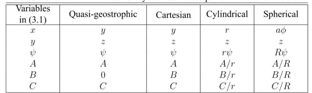
Table (1) tells us how to replace x, y, A, B, and C in (3.1) to morph into different equations.

(3.1) is solved by relaxation method in this study.

Derivative along x and y directions at grid point (i, j) are discretized as

∂ (· )

∂x = (· )_i+1/2,j − ( · )_i_−1/2,j

∆x , (3.3a)

∂ (· )

∂y = (· )_i,j+1/2− ( · )_i,j_−1/2

∆y , (3.3b)

where ∆x and ∆y are grid spacings.

Table 1: General form of Eliassen-Sawyer circulation equation in different coordinates Variables

in (3.1) Quasi-geostrophic Cartesian Cylindrical Spherical

x y y r aϕ

y z z z z

ψ ψ ψ rψ Rψ

A A A A/r A/R

B 0 B B/r B/R

C C C C/r C/R

平衡渦旋模型之熱與動量動力效率

國立臺灣大學理學院大氣科學系 碩士論文

Department of Atmospheric Science College Science

National Taiwan University Master Thesis

平衡渦旋模型之熱與動量動力效率

Dynamic Efficiency of Heat and Momentum in Balanced Vortex Model

許天耀 Tien-Yiao Hsu

指導教授：郭鴻基博士 Advisor: Hung-Chi Kuo, Ph.D.

中華民國 104 年 7 月

July, 2015

誌謝

摘要

ABSTRACT

CONTENTS

LIST OF FIGURES

LIST OF TABLES

CHAPTER 1

INTRODUCTION

CHAPTER 2

FORMULATION

2.1 Efficiency in Quasi-geostrophic Theory

Derivation

Concluding Remarks

2.2 Efficiency in Cartesian Coordinates

Derivation

Concluding Remarks

2.3 Efficiency in Cylindrical Coordinates

Derivation

Concluding Remarks

2.4 Efficiency in Spherical Coordinates

Derivation

Concluding Remarks

2.5 Efficiency in Shallow Water Model

Derivation

Concluding Remarks

CHAPTER 3

NUMERICAL METHOD

國立臺灣大學理學院大氣科學系碩士論文