在有限記憶體下學習的區塊最小化框架

(1)

國立臺灣大學電機資訊學院資訊工程學系碩士論文

Department of Computer Science and Information Engineering College of Electrical Engineering and Computer Science

National Taiwan University Master Thesis

在有限記憶體下學習的區塊最小化框架

Block Minimization Framework for Learning with Limited Memory

林善偉 Shan-Wei Lin

指導教授：林守德博士 Advisor: Shou-De Lin, Ph.D.

中華民國 105 年 07 月 July, 2016

(2)

(3)

摘要

我們考慮在有限記憶體中的最小經驗風險 (Empirical Risk Minimiza- tion) 問題。我們提出一個區塊最小化框架來解決有限記憶體中的四種情況。第一種情況是資料 (data) 比模型 (model) 大而且對偶函式不是平滑的。這個情況在現在的大資料的趨勢當中很容易遇到，當問題的正則項 (regularizer) 是二範數 (norm) 的平方時，就會是這種情況，像是二範數支持向量機 (support vector machine)、二範數邏輯回歸 (logistic regression) 以及二範數線性回歸。第二種情況是資料比模型大但是在對偶函式中存在一項是無法被區塊分割且不平滑的，這種情形發生在範數不是二範數的平方時，這種問題包括一範數線性回歸問題、矩陣填補中的核範數 (nuclear norm) 以及群範數 (group norm) 家族。第三種情況是模型比資料大，而且問題函式在不可切成區塊的部分是平滑的，

這種情況會出現在極端分類問題 (extreme classification) 裡，因為這種問題有非常多類 (class) 以及非常高維度的特徵 (feature) 向量，稀疏編碼 (sparse coding) 也會出現特徵值比資料多的情況，也就是模型比資料大。第四種情況是模型比資料大，但是問題函式中有不可區塊分割的部分同時也不平滑，支持向量機的合頁損失 (hinge loss) 函式就會造成這種情況。在這篇論文裡，我們假設資料或是模型其中之一因為太大而不能全部放進記憶體當中，而另外一個可以放進記憶體中。當資料比較大的時候，我們用對偶區塊最小化方法來解，當模型比較大的時候，我們則用原始 (primal) 區域最小化。在原始區域最小化當中，我

(4)

們把模型分割成很多個區塊，把這些區塊存在硬碟中，每次讀取一個區塊來解，並且只更新這個區塊的參數。而在對偶最小化問題時，我們把資料切成很多塊，把這些區塊存在硬碟，一次讀取一個區塊的資料來做最小化。當有無法被區域分開而且不平滑的項存在時，我們使用拉格朗日增強法使得那一項變成平滑項，來保證最後會收斂到全局最佳解 (global optimum)。當在做原始區塊最小化時，我們在對偶問題加上一個強凸 (strongly convex) 項，使得原始問題變的平滑; 而在做對偶區塊最小化時，我們在原始問題加上一項強凸項，使得對偶問題變平滑。而這多加的一項在演算法接近最佳解的時候會消失，所以我們的方法會收斂到和那些在足夠記憶體下的方法一樣的解。我們的這個框架是靈活的，因為給定一個在足夠記憶體下的解決方法，我們可以只在解決方法上加上一項，就能很容易的把這個解決方法用在有限記憶體之下。

(5)

Abstract

We consider the regularized Empirical Risk Minimization (ERM) in the limited memory environment. We provide a block minimization framework to deal with four situations when training with limited memory. First, when data is larger than the model and the terms in dual objective function are either smooth or block separable. This situation happens frequently in the recently big data trend with L2-regularizer, including L2 Support Vector Ma- chine (SVM), L2 Logistic Regression, and L2 Linear Regression. Second, when data is larger than the model and the non-separable part of dual objective function is non-smooth. It could happen when the regularizer is not L2 norm, including L1-regularizer in Lasso problem, nuclear norm in matrix completion problem, and a family of structure group norms. Third, when model is larger than the data and the terms in primal objective function are either smooth or block separable. This situation appears sometime in the extreme classification problem, which will have large model due to large number of classes and large number of features. Sparse coding is another area that the number of features is larger than the number of samples. Fourth, when model is larger than the data and the non-separable part of primal objective function is non-smooth. Multi-class SVM is an example of this situation, Hinge Loss causes the non-smoothness of the primal objective function. In this paper, we assume that either model or data is too large to fit into memory, and that the

(6)

other one can fit into memory. We use dual block minimization to solve the problem when the data size is larger than the memory size, using primal block minimization to solve it when the model size is larger than the memory. To be specific, in the primal block minimization framework, we split the model into several blocks, store the model in the disk, sequentially load part of the model into memory and update this part only, write this part back to the disk, and read the next part. In the dual block minimization framework, we split data in to blocks and store it in the disk, sequentially load part of the data into memory, update the parameters base on this partial data, than load the next block of data. Also, we apply Augmented Lagrangian technique to force the smoothness of the corresponding objective function when it is non-smooth and non-block-separable to achieve global convergence for the general convex ERM problem. In particular, in the primal block minimization case, we add a strongly convex term to the dual objective in order to force the primal objective function to be smooth. In the dual block minimization case, we add a strongly convex term to the primal problem. This additional term will disappear when the model converge to near the optimal point. Therefore, this algorithm will converge to the same point achieved by the algorithm with sufficient memory. This framework is flexible in the sense that, given a solver working under sufficient memory, one can integrate it into our framework with additional term in the update rule if necessary and obtain a solver globally convergent under limited memory condition.

Keywords: Machine Learning, Limited Memory, Augmented Lagrangian, Empirical Risk Minimization.

(7)

List of Figures

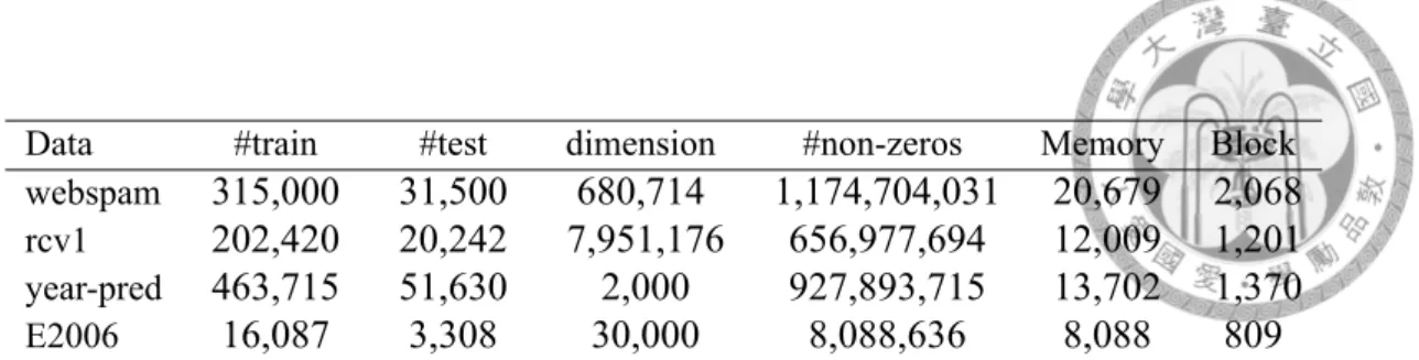
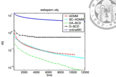
5.1 Objective Value for Webspam data set . . . 31

5.2 Error for Webspam data set . . . 32

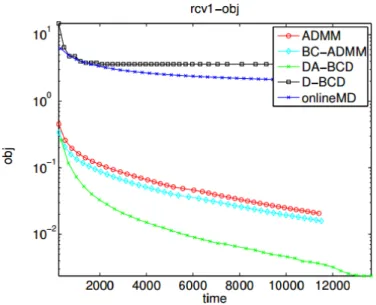
5.3 Objective Value for Rcv1 data set . . . 32

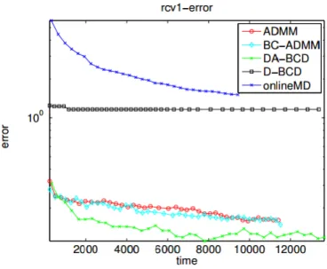
5.4 Error for Rcv1 data set . . . 33

5.5 Objective Value for Year-pred data set . . . 33

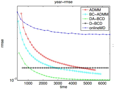
5.6 RMSE for Year-pred data set . . . 34

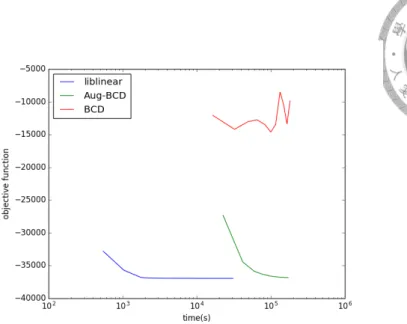
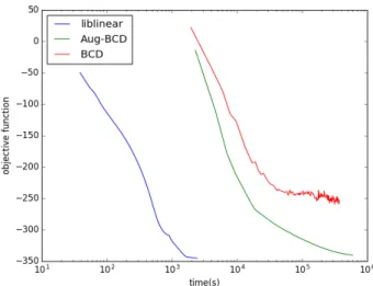
5.7 Objective Value for E2006 data set . . . 34

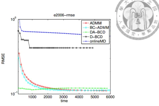
5.8 RMSE for E2006 data set . . . 35

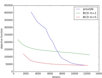
5.9 Objective Value for LSHTC1 data set on LR . . . 37

5.10 Objective Value for aloi.bin data set on LR . . . 37

5.11 Objective Value for LSHTC1 data set on SVM . . . 38

5.12 Objective Value for aloi.bin data set on SVM . . . 39

(10)

(11)

List of Tables

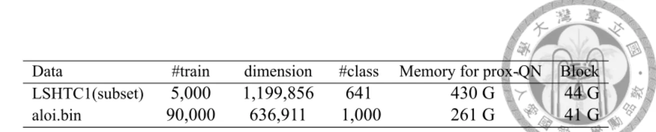
5.1 Data Statistic for Dual Augmented BCD . . . 30 5.2 Data Statistic for L1-regularized Multi-class Logistic Regression . . . 36 5.3 Data Statistic for L2-regularized Multi-class SVM . . . 36

(12)

(13)

Chapter 1 Introduction

Nowadays, there are many applications of machine learning and data mining trained by data with huge scale. It has been observed that model’s performance can be boosted by increasing both the number of samples and the number of features. With the help of crowd- sourcing, data with million number of features and number of samples was generated[3].

As a consequence, data size can easily exceed the size of memory, we cannot load whole data or model into memory and have to use the secondary storage when training a model.

Therefore, we have to consider the expensive I/O time and balance with computational time during training.

There are two disparate ways will be considered when training a model with huge data, online and distributed learning. In the online learning scenario, each sample is processed only once in a stochastic manner without being stored. The drawback of online learning is that it require large number of epochs to converge to the same level of batch method. If we want to obtain a useful result, we still have to memorize all the data in disk and process it to memory several times during training, and the algorithm spends most of the time in I/O instead of computation at each epoch; therefore, the bottleneck in the online learning setting is I/O[2, 22, 25]. The problem of slow convergence for an online algorithm will become even much worse for non-smooth or non-strongly convex objective function [16, 18]

(14)

than the strongly convex problem like L2-regularized SVM [15]. In the distributed learning setting, there are many cores or machines that can process data at the same time and jointly fit the data into memory. However, in the real case, there may not have sufficient number of machines to store the whole data into memory. In this situation, the algorithm can only process a block of data at a time. Therefore, we will also encounter large number of I/O and have to consider the I/O time in the distributed learning setting[25].

Recently, several algorithms have been proposed to solve large-scale linear Support Vector Machine (SVM) in the limited memory setting[2, 22, 25]. These approaches are based on a dual Block Coordinate Descent (dual-BCD) algorithm, which split the original problem into several block sub-problems, each sub-problem only requires a block of data loaded into memory. As a result, the machine will process a block of data from disk to memory when changing the block sub-problem, allowing more computation between two I/O and balance the computation time and the I/O time. This approach was proved linear convergent to global optimum, and showed fast convergence in the experiment. However, the global convergence for dual-BCD method base on the assumption that the non-separable part of the dual problem is smooth, which is not the case in the general Empirical Risk Minimization (ERM) problem except the regularizer is L2-norm.

Another scenario in the limited memory setting is that the model size is larger than the memory size, we assume that the data size is smaller than the memory size. This scenario may happen in the extreme classification problem, the model can easily become very large when both number of features and the number of classes are large. Another application is Sparse Coding, which usually has extremely large number of features and smaller number of samples[7], and some problems require the memory size equal to square of the number of features, such as inverse covariance estimation problem. Traditional algorithms which requires the whole model to process is infeasible. We can apply the same technique discuss above, except that we apply BCD based on the primal problem instead of dual problem. The primal BCD method separates model into blocks and update one block at

(15)

a time, we only need a block of model loaded in the memory to perform the algorithm.

This method achieves linearly convergent when the loss function is strongly convex[14].

However, primal-BCD will not converge to the global optimum if the non-separable part of the primal objective function is non-smooth.

In this paper, we propose a general framework to solve the regularized Empirical Risk Minimization problem (ERM) in the limited memory setting, which include the situation that the data is larger than the memory and that the model is larger than the memory. ERM problem covers most of supervised learning problems ranging from classification, regression, ranking and recommendation, many of them have non-separable and non-smooth part in primal objective function or dual objective function, leading to the result that BCD method cannot converge to global optimum. Then we discuss the convergence issue and then apply Proximal Point method to allow the algorithm’s global convergence.

We conduct experiments on the L1-regularized classification and regression problems when data is larger to corroborate our theory, which shows the proposed augmented technique improve the convergence dramatically. We also provide another general framework in limited memory setting adapted from a famous distributed method Alternating Direc- tion Method of Multiplier (ADMM)[1]. The experiments show that the adaptive ADMM is efficient but not as efficient as the proposed framework specially designed for limited memory setting.

We experiment on multi-class classification problems with both smooth loss function and non-smooth loss function when model size is larger than the data size and the memory size, which will happen when the number of features is larger than the number of samples and the number of classes is huge. we show that one can reduce the memory usage almost linearly with the number of blocks during training, and the proposed algorithm indeed converge to the same point that the original algorithm converge to.

Note that we didn’t compare our method with the recently proposed distributed learning algorithms (CoCoA etc.)[9, 8], because they can only apply to L2 regularized ERM prob-

(16)

lems or designed for some specific loss function, such as L1-logistic regression[20].

The recently proposed distributed learning algorithm PROXCoCoA⁺[17] which can deal with more general regularizer is similar to our framework. However, their framework aims to deal with the ERM problem in the distributed system, instead of saving memory as the framework we proposed. Furthermore, if we adopt PROXCoCoA⁺ to limited memory setting like ADMM, it will be the same with our framework except that PROXCoCoA⁺ has shrinked step size, which is required to guarantee convergence. Therefore, we didn’t compare it with our method.

(17)

Chapter 2 Problem Setup

In this work, we consider the regularized Empirical Risk Minimization problem, which given a data set D ={(ϕn, y_n)}^N_n=1, estimates a model through

min

w∈R^d,ξ∈R^pF (w, ξ) = R(w) +

∑N n=1

L_n(ξ_n)

s.t.ϕ_nw = ξ_n, n∈ [N]

(2.1)

where w∈ R^dis the model parameters to be estimated, ϕ_nis a p by d design matrix that encodes features of the n-th data sample,L_n(.) is a convex loss function that penalizes the difference between ground truth and prediction vector ξ_n ∈ R^p, and R(w) is a convex regularized function preventing overfitting.

The formulation (2.1) cover a large class of statistical learning problems ranging from classification [26], regression [19], ranking [10], and convex clustering [21]. For example, in classification problem, we have p =|Y | where Y consists the set of all labels, we can use logistic loss L_n(ξ) = log(∑

k∈Y exp(ξ_k)− ξyn) in logistic regression and hinge loss L_n(ξ) = max_k_∈Y(1− δk,yn + ξ_k− ξyn) in support vector machine; in a (multi-task) regression problem, there are K real values for the target variable Y , we have p = K, and the square loss L_n(ξ) = ¹₂||ξ − yn||²2 is often used. There are various regularizers

(18)

R(w) used in different applications, which includes the L2-regularizer R(w) = ^λ₂||w||² in ridge regression and many classification problems, L1-regularizer R(w) = λ||w||1 in Lasso, nuclear norm R(w) = λ||w||∗ in matrix completion, and a family of structure group norms R(w) = λ||w||g [12]. These variety functions of R(w), L_n(ξ) differ in two properties – strongly convexity and smoothness – that dramatically affect the convergence behavior of the block minimization algorithm.

Definition 1 (Strongly Convexity). A function f (x) is strongly convex iff it is lower bounded by a simple quadratic function

f (y)≥ f(x) + ∇f(x)^T(y− x) + m

2||x − y||² (2.2)

for some constant m > 0 and∀x, y ∈ dom(f).

Definition 2 (Smoothness). A function f (x) is smoothness iff it is upper bounded by a simple quadratic function

f (y) ≤ f(x) + ∇f(x)^T(y− x) + M

2 ||x − y||² (2.3)

for some constant 0 ≤ M < ∞ and ∀x, y ∈ dom(f). For instance, the square loss and logistic loss are both smooth and strongly convex ¹, while the hinge loss satisfies neither of them. Moreover, L2-norm is the only regularizer that is both strongly convex and smooth, other regularizer such as L1-norm, structured group norm, and nuclear norm have neither of these two properties. We will demonstrate the effects of these properties to Block Minimization algorithms.

Throughout this paper, we will assume that given a solver for the ERM problem (2.1) that works in the condition that the model and the data can fit in memory, we can easily integrate the solver into our framework, and the framework can efficiently solve (2.1)

1The logistic loss is strongly convex when its input ξ are within a bounded range, which is true as long as we have a non-zero regularizer R(w)

(19)

when data cannot fit into memory or model cannot fit into memory. We will also assume that either model or data can fit into memory when another one cannot in the limited memory condition. In the following sections, we will abbreviate the condition that data cannot fit in memory as large data condition, and the condition that model cannot fit into memory as large model condition.

(20)

(21)

Chapter 3 Primal and Dual Block Minimization

In this section, we will first extend the block minimization framework of [25] from linear L2-regularizer SVM to the general setting of regularized ERM problem (2.1) in the large data scenario. Then we will discuss the block minimization framework for regularized ERM problem in the condition that model cannnt fit in memory.

3.1 Data Size is Larger than The Memory Size

For the large data condition, we apply dual-BCD to ERM problem, the dual form of equation (2.1) can be expressed as

min

µ∈R^d,αn∈R^pR^∗(−µ) +

∑N n=1

L^∗_n(α_n)

s.t.

∑N n=1

ϕ^T_nα_n= µ

(3.1)

where R^∗(−µ) is the convex conjugate of R(w) and L^∗n(α_n) is the convex conjugate of L_n(ξ_n). The convex conjugate is defined as follow

Definition 3 (Convex Conjugate). Given a convex function f : χ→ R∪{∞}, the convex

(22)

conjugate f^∗ : χ→ R ∪ {∞} is defined as

f^∗(y) := sup

x∈χ⟨x, y⟩ − f(x) (3.2)

where⟨·, ·⟩ denotes the inner product in a Euclidean vector space χ.

The block minimization framework of [25] basically performs a dual-BCD over (3.1) by dividing the whole data set D into K blocks D_B₁, ..., D_B_K, and optimize a block of dual variables (α_B_k, µ) at a time, where D_B_k ={(ϕn, y_n)}n∈Bk and α_B_k ={αn|n ∈ Bk}.

In [25], the dual problem (3.1) is derived explicitly and solved in the dual function in order to perform the algorithm. However, for many sparsity-inducing regularizer such as L1-norm and nuclear norm, it is more efficient and convenient to solve in primal function [6, 27]. Therefore, here we express the dual problem implicitly as

G(α) = min

w,ξ L(α, w, ξ)

= min

w,ξ R(w) +

∑N n=1

Ln(ξ_n) +

∑N n=1

α^T_n(ϕ_nw− ξn)

(3.3)

whereL(α, w, ξ) is the Lagrangian function of equation (2.1). Then we maximize (3.3) w.r.t a block of dual variables αB_kwith other dual variables{αBj = α^t_B

j}j̸=kfixed, where t denotes the iteration of the BCD algorithm. By strong duality,

maxα_Bk

{

minw,ξ L(α, w, ξ) }

= min

w,ξ

{

maxα_Bk L(α, w, ξ) }

= min

w,ξ F_B_k(w, ξ) (3.4)

we can form a primal sub-problem for each block. The maximization of dual variables α_B_k in (3.4) enforces the primal equalities ϕ_nw = ξ_n, n∈ Bk, resulting the block mini-

(23)

mization primal problem

min

w∈R^d,ξ∈R^pF_B_k(w, ξ) = R(w) +

∑N n=1

L_n(ξ_n) + µ^t_B

k

Tw

s.t.ϕ_nw = ξ_n, n∈ Bk

(3.5)

where µ^t_B

k =∑

n /∈Bkϕ^T_nα^t_ndenotes the information of other blocks that affects the value of global function (2.1). Note that in (3.5), variables{ξn}_{n /}_∈B_k have been dropped since they are not relevant to the dual variables in this block α_B_k. Therefore, given the d dimen- sional vector µ^t_B

k, we can solve (3.5) without the data of other blocks{(ϕn, y_n)}_{n /}_∈B_k. In the algorithm, we maintain a d dimensional vector µ^t =∑N

n=1ϕ^T_nα^t_nand obtain µ^t_B

k by

µ^t_B

k = µ^t− ∑

n∈Bk

ϕ^T_nα^t_n (3.6)

to solve each block subproblem (3.5). A convenient property for the subproblem (3.5) is that it has the same form of the original problem (2.1) except for one additional linear augmented term µ^t_B_k^Tw. Given a solver of (2.1), we can easily adapt the solver to solve (3.5) by adding an augmented term for the gradient

∇wF_B_k(w, ξ) =∇wF (w, ξ) + µ^t_B

k

of the solver, where F_B_k(·) denotes the subproblem function and F (·) denotes the original function. Note that the augmented term µ^t_B

k is constant and separable w.r.t. coordinate, so it takes little overhead to the solver. After obtaining the solution (w^∗, ξ^∗_B

k) from (3.5), we can compute the corresponding dual variables α_B_k according to the KKT condition and maintain µ by

α^t+1_n =∇ξ_nL_n(ξ^∗_n), n∈ Bk (3.7)

µ^t+1_n = µ^t_B_k + ∑

n∈Bk

ϕ^T_nα^t+1_n (3.8)

(24)

The procedure is summarized in Algorithm 1, which consumes O(d +|DB_k| + p|Bk|) memory capacity. The factor d comes from the storage of the vector µ^t, w^t, factor|DBk| comes from the storage of data block, and the factor p|Bk| comes from the storage of α_B_k. Note that this algorithm requires the same space complexity as that require in the original algorithm proposed for linear SVM [25], where p = 1 for the binary classification problem.

Algorithm 1 Dual Block Minimization

Require: Split dataD into blocks B1, B₂, ...B_K.

1: Initial µ⁰ = 0.

2: for t=0,1,... do

3: Draw k uniformly from [K].

4: LoadDB_k and α^t_B_k into memory.

5: Compute µ^t_B

k from (3.6).

6: Solve (3.5) to obtain (w^∗, ξ^∗_B

k).

7: Compute α^t+1_B

k from (3.7).

8: Maintain µ^t+1by (3.8)

9: Save α^t+1_B

k out of memory.

3.2 Model Size is Larger than The Memory Size

For the large model condition, we perform primal-BCD to ERM problem (2.1). We first split model w into K blocks w_B₁, ...w_B_K, and optimize a block of primal variables w_B_k at a time, where w_B_k ={wi|i ∈ Bk} indicate the parameters in this block. We derive the subproblem from LagrangianL(α, w, ξ) by minimizing a block of primal variables wB_k

maxα

{ min

w_Bk,ξL(α, w, ξ) }

= max

α G_B_k(α) (3.9)

with parameters in other blocks {

w_B_j = w^t_B

j

}

j̸=k fixed, again t is the iteration of the primal-BCD algorithm. The minimization of primal variables w_B_k in (3.9) enforces the dual equality ∑N

n=1ϕ^T_n,iα_n = µ_i, i ∈ Bk, which resulting in the block minimization

(25)

problem

min

µ_Bk∈R^d/K,αn∈R^pR^∗(−µBk) +

∑N n=1

L^∗_n(α_n)− δ^tn,Bk

Tα_n

s.t.

∑N n=1

ϕ^T_n,B

kα_n = µ_B

k

(3.10)

where ϕ_n,B

k = {

ϕ_n,i|i ∈ Bk

} denotes the feature of the n-th data which have the same

dimension of the parameters in this block B_k, µ_n,B

k = {

µ_n,i|i ∈ Bk

}, and δ^t_n,B

k =

{ϕ_n,iw^t_i}

i /∈Bk. Note that in (3.10), variables{R(wi)}_{i /}_∈B_k have been dropped since they have no effect to the block subproblem. Given the p dimensional vector δ_n,B_k for each sample, we can solve (3.10) without the parameters outside the block B_k. Same as the dual-BCD algorithm, we maintain p dimensional vector δn= ϕ_nw^tand obtain δn,B_k by

δ^t_n,B

k = δ^t_n− ϕn,Bkw^t_B

k (3.11)

to solve the block subproblem (3.10). After obtaining solution (α^∗) from (3.10), we are able to derive the corresponding optimal primal variable wB_k for (3.9) according to the KKT condition and maintain δ_nby

w^t+1_B

k =

( _N

∑

n=1

ϕ_n,B_k

)−1∑N

n=1

∇αnL^∗_n(α^∗_n) (3.12)

δ^t+1_n = δ^t_n,B

k+ ϕ_n,B_kw^t+1_B

k (3.13)

Note that we can modify the original solver for (3.1) easily by adding an augmented term to the original gradient

∇αG(α) =˜ ∇αG(α)− δ^tBk

where ˜G(·) denotes the subproblem (3.10) and G(·) denotes the original problem (3.1).

(26)

3.2.1 Solve Block SubProblem in Primal

We also can form a primal subproblem for the above primal-BCD algorithm, for the convenient of solving with many sparsity-inducing regularizer such as L1-norm and nuclear norm. By strong duality, the subproblem (3.9) can be express as

maxα

{

wmin_Bk,ξL(α, w, ξ) }

= min

w_Bk,ξ

{

maxα L(α, w, ξ)}

= min

w_Bk,ξF_B_k(w, ξ) (3.14)

The maximization of dual variables α enforces the primal equation ϕ_nw = ξ, resulting a subproblem

wmin_Bk,ξF_B_k(w, ξ) = min

w_Bk,ξR(w_B_k) +

∑N n=1

L_n(ξ_n)

s.t.ϕ_n,B

kw_B_k = ξ_n− δn,Bk, n∈ [N]

(3.15)

which can directly output w^t+1_B

k without computing α^∗.

The overall procedure for primal-BCD is summarized in Algorithm 2, which requires O(|Bk| + D + p × n) space complexity. The factor |Bk| comes from the storage of model block w_B_k, the factorD comes from the storage of data, and the factor p × n comes from the storage of α_n, δ^t_n.

Algorithm 2 Primal Block Minimization

Require: Split model w into blocks B₁, B₂, ...B_K.

1: Initial δ⁰ = 0.

2: for t=0,1,... do

4: Load w_B_k into memory.

5: Compute δ^t_B

k from (3.11).

6: Solve (3.10) to obtain (α^∗) and compute w^t+1_B

k from (3.12)

7: (or solve (3.15) to obtain w^t+1_B

k )

8: Maintain δ^t+1by (3.13)

9: Save w^t+1_B

k out of memory.

(27)

Chapter 4 Augmented Block Minimization

Although the Block Minimization Algorithm 1 and 2 can be applied to the general regularized ERM problem (2.1), it is not guaranteed that the sequence{α^t}^∞_t=1 and{w^t}^∞_t=1 generated by Algorithm 1 and Algorithm 2 respectively converge to global optimum of (2.1). In fact, the global convergence of Algorithm 1 and Algorithm 2 only happens for some special function. One sufficient condition for the global convergence of a Block- Coordinate Descent algorithm is that the terms in objective function that are not separable w.r.t. blocks have to be smooth(Definition 2).

First, we examine the dual objective function (3.1), which contains two terms R^∗(−∑_N

n=1ϕ^T_nα_n)+

∑_N

n=1L^∗_n(α_n), where the second term is separable w.r.t. samples{αn}^Nn=1, thus it is separable w.r.t. blocks{αBk}^K_k=1. However, the first term couples dual variables in all the blocks and it is not separable w.r.t. blocks. Therefore, if R^∗(·) is smooth, Algorithm 1 will converge to global optimum. The following theorem suggests that it will happen only when R(w) is strongly convex.

Theorem 4.0.1 (Strong/Smooth Duality). Assume f (·) is closed and convex. Then f(·) is smooth with parameter M if and only if its convex conjugate f^∗(·) is strongly convex with parameter m = _M¹

The proof of above theorem can be found in [11]. According to theorem 4.0.1, the

(28)

dual-BCD Algorithm 1 will guarantee to have global convergence only when the regu- larizer is L2-norm R(w) = ¹₂||w||². Unfortunately, most of regularizers is not strongly convex, thus the dual-BCD algorithm failed to converge to global minimum in most of the regularizers and many applications.

Then we consider the primal-BCD algorithm, the primal objective function (2.1) consist of two terms R(w) +∑N

n=1L_n(ϕ_nw). The first term is separable w.r.t. coordinate for L1-norm and L2-norm, hence it is separable w.r.t. blocks. There are many more choice of regularizers such as group lasso, sparse group lasso, and nuclear norm that are block separable. For the second term, although the logistic loss and square loss is smooth, there is a popular loss function called hinge loss L_n(ξ) = max_k_∈Y(1− δk,y+ ξ_k− ξyn) which appears in the SVM model that is non-smooth. Therefore, Algorithm 2 is not globally convergent for SVM.

In this section, we propose a solution to this problem for both dual and primal BCD. We apply Proximal Point method to the subproblem, generating the smoothness for the non- smooth and non-separable term. As a result, both dual and primal BCD algorithm has fast global convergence.

4.1 Algorithm

The Proximal Point Method (or equivalently, Dual Augmented Lagrangian method) mod- ifies the original problem by introducing a sequence of Proximal Maps

w˜^t+1 = arg min

w

F (w) + 1

2η_t||w − ˜w^t||² (4.1)

to iterative achieve optimum, where F (w) denotes the ERM problem (2.1). We will first demonstrate how to modify the dual-BCD algorithm, and then apply the same technique to primal-BCD algorithm.

(29)

4.1.1 Dual Augmented Block Minimization

In this section, we extend the algorithm in section 3.1. We perform dual-BCD algorithm on the proximal problem (4.1) instead of solving the original subproblem (3.5). As we show in the analysis section, the dual problem of (4.1) is globally convergent since the non- separable terms for the dual variables α_B_k are smooth. Given the current iterate model

˜

w^t, the Dual Augmented Block Minimization optimize one block of the dual variables α_B_k of proximal point problem (4.1) at a time, with other variables fixed

{

α_B_j = α^(t,s)_B

j

}

j̸=k, where t denotes the number of iteration of proximal point method, and s denotes the num- ber of iteration of inner dual-BCD method. By strong duality,

maxα_Bk

{ min

w,ξ

L(α, w, ξ)˜ }

= min

w,ξ

{ maxα_Bk

L(α, w, ξ)˜ }

(4.2)

where ˜L(·) is the Lagrangian of (4.1)

L(α, w, ξ) = F (w, ξ) +˜

∑N n=1

α^T_n(ϕ_nw− ξn) + 1

2η_t||w − ˜w^t||² (4.3)

Once again, we maximization w.r.t. α_B_k enforces the primal equalities for this block ϕ_nw = ξ_n, n∈ Bkand form a primal subproblem

min

w∈R^d,ξ∈R^pR(w) +

∑N n=1

L_n(ξ_n) + µ^(t,s)_B

k

Tw + 1

2η_t||w − ˜w^t||² s.t.ϕ_nw = ξ_n, n∈ Bk

(4.4)

where µ^(t,s)_B

k =∑

n /∈Bkϕ^T_nα^(t,s)n . Note that (4.4) is almost the same as (3.5) except the ad- ditional proximal point term. We follow the same procedure to maintain the d dimensional vector µ^(t,s)=∑_N

n=1ϕ^T_nα^(t,s)n and obtain

µ^(t,s)_B

k = µ^(t,s)− ∑

n∈Bk

ϕ^T_nα^(t,s)_n (4.5)

(30)

to be able to solve the block subproblem (4.4). After obtaining the solution (w^∗, ξ^∗_B_k) from (4.4), we derive dual variables α_B_k as

α^(t,s+1)_n =∇ξ_nL_n(ξ^∗_n), n∈ Bk (4.6)

and maintain µ as

µ^(t,s+1)_n = µ^(t,s)_B

k + ∑

n∈Bk

ϕ^T_nα^(t,s+1)_n (4.7)

The block subproblem (4.4) is similar to the original ERM problem (2.1) with additional simple quadratic augmented function which is separable w.e.t. coordinate. Given a solver of (2.1) working in sufficient memory condition, we can easily modify it to

∇wF˜_B_k(w, ξ) =∇wF (w, ξ) + µ^(t,s)_B

k +w− ˜w^t η_t

∇²wF˜_B_k(w, ξ) =∇²wF (w, ξ) + I η_t

where ˜F_B_k(·) denotes the proximal point block subproblem, F (·) denotes the original objective function. The inner Block Minimization procedure is performed until every value of subproblem (4.4) reaches ϵ_in from the optimum. Then the outer proximal point method update ˜w^t+1= w^∗(α^(t,s)) is performed, where w^∗(α^(t,s)) is the solution of (4.4) for the latest inner iteration s, and the corresponding dual variables is α^(t,s). The overall procedure is summarize in Algorithm 3.

4.1.2 Primal Augmented Block Minimization

In this section, we show how to apply the Proximal Point Method to the primal-BCD algorithm, extending the algorithm in section 3.2. We introduce a sequence of Proximal Maps in the dual problem

˜

α^t+1= arg min

α

G(α) + 1

2η_t||α − ˜α^t||² (4.8)

(31)

Algorithm 3 Dual-Aug. Block Minimization Require: Split dataD into blocks B1, B₂, ...B_K.

1: Initial µ⁰ = 0, ˜w⁰ = 0.

2: for t=0,1,... do

3: for s=0,1,...S do

5: LoadDBk and α^(t,s)_B

k into memory.

6: Compute µ^(t,s)_B

k from (4.5).

7: Solve (4.4) to obtain (w^∗, ξ^∗_B

k).

8: Compute α^(t,s+1)_B

k from (4.6).

9: Maintain µ^(t,s+1)by (4.7)

10: Save α^(t,s+1)_B

k out of memory.

11: w˜^t+1 = w^∗(α^(t,S+1))

where G(α) denotes the dual of ERM problem (3.1). We perform primal-BCD on the dual proximal problem (4.8) instead of the original ERM problem (2.1). The algorithm will converge to global optimum since the non-smooth loss L_n(·) which is not block separable will become smooth by adding the proximal term ||α − ˜α^t||². Given the current dual iterate variables ˜α^t, which t is the number of outer iteration, the Primal Augmented Block Minimization algorithm optimizes the primal variables w_B_kin one block B_kat a time, and other primal variables

{

w_B_j = w^(t,s)_B

j

}

j̸=k are fixed, where s denotes the number of inner BCD iteration.

maxα

{

wmin_Bk,ξ

L(α, w, ξ)˜ }

= max

α GB_k(α) (4.9)

where ˜L(α, w, ξ) is the Lagrangian of (4.8)

L(α, w, ξ) = F (w, ξ) +˜

∑N n=1

α^T_n(ϕ_nw− ξn)− 1

2η_t||α − ˜α^t||² (4.10)

Note that there is a minus sign in front of the proximal term in (4.10), since we maximize the Lagrangian w.r.t. dual variables instead of minimizing in the problem (4.8). The maximization of (4.9) enforce the equality∑N

n=1ϕ^T_n,iα_n = µ_i, i∈ Bk, leading to a block

(32)

minimization subproblem

min

µ_Bk∈R^d/K,αn∈R^pR^∗(−µB_k) +

∑N n=1

L^∗_n(α_n)− δ^(t,s)_n,B_k^Tα_n+ 1

2η_t||α − ˜α^t||² s.t.

∑N n=1

ϕ^T_n,B_kα_n= µ_B_k

(4.11)

where δ^(t,s)_n,B

k = {

ϕ_n,iw^(t,s)_i }

i /∈Bk

. Note that (4.11) is the primal-BCD subproblem (3.10) with an augmented proximal point term. We have the some procedure to maintain δ^(t,s)_n = ϕ_nw^(t,s)and to update δ^(t,s)_n,B

k by

δ^(t,s)_n,B

k = δ^(t,s)_n − ϕn,Bkw^(t,s)_B

k (4.12)

in order to solve the subproblem (4.11). After we obtain the solution α^∗ from (4.11), we can update primal variables wB_k as

w^(t,s+1)_B

k =

( _N

∑

n=1

ϕ_n,B_k

)−1∑N

n=1

∇αnL^∗_n(α^∗_n) (4.13)

and maintain δ_nas

δ^(t,s+1)_n = δ^(t,s+1)_n,B

k + ϕ_n,B

kw^(t,s+1)_B

k (4.14)

Note that we can modify the original solver for (3.1) easily by adding an augmented term to the original gradient

∇αG(α) =˜ ∇αG(α)− δ^(t,s)Bk +α− α^t η_t

∇²_αG(α) =˜ ∇²_αG(α) + I η_t

where ˜G(·) denotes the subproblem (4.11) and G(·) denotes the original problem (3.1).

(33)

Solve Subproblem in Primal

Once again, we can solve the above subproblem (4.11) in the primal form for the convenient of solving sparsity-inducing regularizer, by strong duality, the subproblem (4.9) can first optimize dual variables

maxα

{ min

w_Bk,ξL(α, w, ξ) }

= min

w_Bk,ξ

{

maxα L(α, w, ξ)}

(4.15)

Resulting a primal subproblem

wmin_Bk,ξR(w_B_k) +

∑N n=1

L_n(ξ_n) + ηt

2

∑N n=1

||(ϕn,Bkw_B_k + δ_n,B_k − ξn)−α˜^t_n

η_t ||² (4.16)

and we can directly obtain w^(t,s)_B

k without compute α^∗.

The inner Block Minimization procedure stop when every subproblem (4.11) (or (4.16)) reaches ϵ_in tolerance. After that, a update of the outer proximal point method ˜α^t+1 = α^∗(w^(t,s))is performed, where α^∗(w^(t,s)) is the solution of (4.11)(or (4.16)) for the latest primal variables w^(t,s). The procedure is summarized in Algorithm 4.