廣義多參數概似模型之估計

(1)

國立臺灣大學理學院數學系(所) 博士論文

Department of Mathematics College of Science

National Taiwan University Doctoral Dissertation

廣義多參數概似模型之估計 On Estimation Methods in Generalized Multiparameter

Likelihood Model

陳律閎 Lu-Hung Chen

指導教授: 鄭明燕教授 Advisor: Prof. Cheng, Ming-Yen

中華民國 99 年 1 月

國立臺灣大學數學系( 所)

博士論文

廣義多參數概似模型之估計

陳

律

閎

撰

99

1

(2)

Abstract

Multiparameter likelihood models (MLMs) with multiple covariates have a wide range of applications; however, they encounter the “curse of dimensionality” problem when the dimension of the covariates is large. We develop a generalized multiparameter likelihood model that copes with multiple covariates and adapts to dynamic structural changes well. It includes some popular models, such as the partially linear and varying-coefficients models, as special cases. We discuss the backfitting and profile likelihood procedures and present a simple, effective two-step method to estimate both the parametric and the nonparametric components when the model is fixed. All these estimators of the parametric component has the n^−1/2 convergence rate, and the estimator of the nonparametric component enjoys an adaptivity property. We suggest a data-driven procedure for selecting the bandwidths, and propose an initial estimator in backfitting and profile likelihood estimation of the parametric part to ensure stability of the approach in general settings. We further develop an automatic procedure to identify constant parameters in the underlying model.

We provide several simulation studies and an application to infant mortality data of China to demonstrate the performance of our proposed method.

(3)

中文摘要

能處理多個共變數(covariate)的多參數概似模型(Multiparameter Likelihood Models, MLMs)有非常廣泛的應用。然而，當共變數的維度很大時，我們會遇到”維度的詛咒(curse of dimensionality)”的問題。我們將多參數概似模型推廣成半參數模型，使之能處理較大的共變數維度同時能適應動態的結構變化。我們的模型包含了許多特例，如部份線性模型(partially linear models)、

變係數模型(varying coeﬃcients models)等。我們介紹兩種既有的方法以及提出一個簡單而且有效的兩步驟估計法來估計此模型的參數化的部份以及非參數的部份。這些估計方式在參數化的部份具有和一般參數化模型一樣的收斂 速度(n^−1/2)，非參數的部份則能估的和已知參數化的部份時一樣好(即具有 adaptivity property)。我們也提了一個自動帶寬選擇(bandwidth selection)法，

以及一個自動化的流程來決定哪些共變數應該被放在參數化的部份。我們做了一些模擬研究，並且舉了一個中國嬰兒死亡率的資料來顯示我們估計方法的性能。

(4)

致謝

首先感謝指導教授鄭明燕老師多年以來費心的指導與栽培，不管是學術上知識的教導還是其對工作、研究的嚴謹與熱誠的身教言教，均給我莫大的影響，讓我獲益良多。沒有鄭老師給我這麼好的題目以及過程中的指導，本研究的進行及論文撰寫不可能如此順利的完成，在此謹致上由衷的謝忱。

另外要感謝曾勝滄老師、戴政老師、張淑惠老師以及丘政民老師首肯擔任我的口試審查委員，給我論文撰寫以及實務研究方面之詳細指正，讓本論文不致犯錯並更加完備。此外，感謝陳祝嵩老師慷慨提供計算資源，使論文得以如期完成。

最後，謹將本論文獻給我的父母，感謝他們的養育之恩及對我永遠的支持、

鼓勵。

(5)

List of Figures

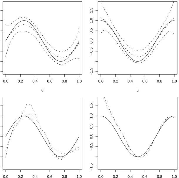
1 Functional parameters in logistic regression when the sample size is

1000 . . . 43

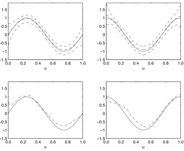
2 Functional parameters in logistic regression when the sample size is 500 . . . 44

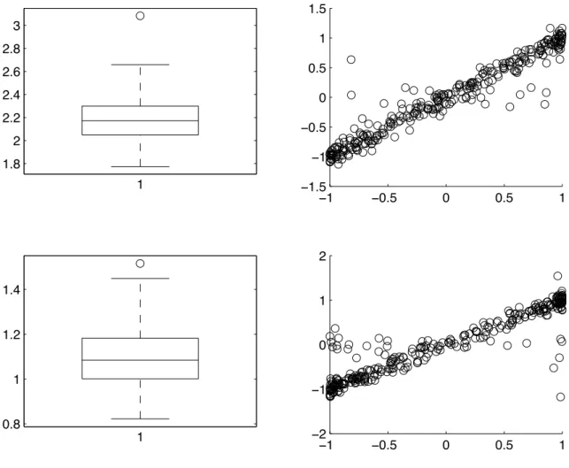
3 Parameter predictions in the logistic example when the sample size is 1000 . . . 46

4 Parameter predictions in the logistic example when the sample size is 500 . . . 47

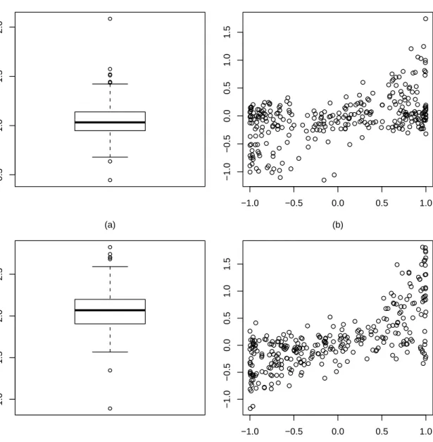
5 Parameter predictions in the logistic example by the AIC criterion when the sample size is 1000. . . 49

6 Parameter predictions in the logistic example by the AIC criterion when the sample size is 500. . . 50

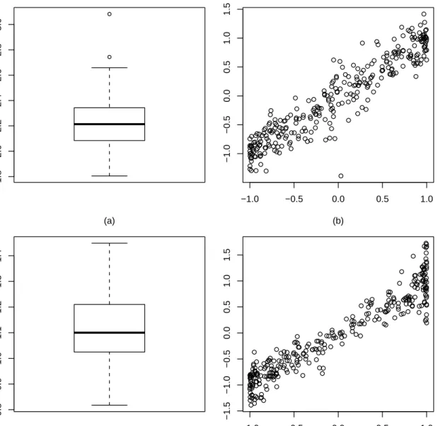
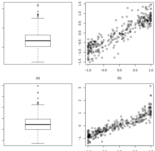
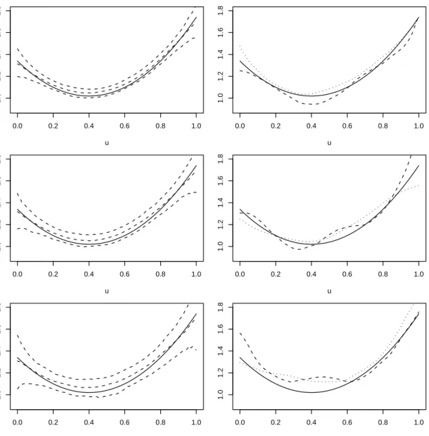
7 Estimates of the functional parameter in the Weibull example. . . 53

8 Parameter predictions in the Weibull example. . . 57

9 Parameter predictions in the Weibull example with the AIC criterion. 59 10 Impacts of covariates on infant mortality with modelM0 . . . 66

11 Impacts of covariates on infant mortality with modelM^′₀ . . . 67

12 Impacts of covariates on infant mortality . . . 70

13 Impacts of covariates on infant mortality with modelM^′ . . . 73

(8)

List of Tables

1 MIAEs of diﬀerent estimation methods for logistic regression. . . 41 2 Performances of diﬀerent estimation methods on the Weibull example

when the sample size is 1000. . . 54 3 Performances of diﬀerent estimation methods on the Weibull example

when the sample size is 500. . . 54 4 Performances of diﬀerent estimation methods on the Weibull example

when the sample size is 250. . . 55 5 Performances of model selection procedures of the Weibull example. . 58 6 Estimated impacts of the constant parameters with modelM and M^′ 74 7 List of Covariates with Descriptive Statistics . . . 75

(9)

1 Introduction

Consider statistical modeling of the relationship between a response variable and some covariates. Maximum likelihood estimation is most powerful when the joint distribution of the response variable and covariates is speciﬁed by a parametric form.

But parametric approaches are at risk for model misspeciﬁcation, which can result in seriously biased estimation, misinterpretation of data, and other problems. Non- parametric modeling is more ﬂexible and allows data to present the unknown truth;

however, it often comes up against the “curse of dimensionality” problem — that is, model instability when the dimension of the covariates is large. Numerous hybrids of parametric and nonparametric models, generally called semiparametric models, have been proposed to achieve a good balance between ﬂexibility and stability in model speciﬁcation. We will review related models in Section 3.

In this article we suggest a semiparametric model for a population (X, U, Y ) in which U is a continuous variable and the conditional density function of Y given (X, U ) is speciﬁed by

f (

Y ; X, θ, x^T₁a₁(U ), · · · , x^T_ℓa_ℓ(U ) )

, (1.1)

where f is a known parametric density function, θ = (θ₁,· · · , θq)^T is an unknown constant vector, X = (X₁,· · · , Xp)^T with X₁ ≡ 1, and xj is a p_j-dimensional subvec- tor of X and a_j(·) = (aj1(·), · · · , ajpj(·))^T is an unknown function, j = 1,· · · , ℓ. Here 1 ≤ ℓ ≤ d, where d is as deﬁned in (1.2). Model (1.1) is a hybrid of the standard

(10)

multiparameter likelihood model (MLM) that assumes that the conditional density function of Y given X follows the form

f (

Y ; a₁(X), · · · , ad(X) )

, (1.2)

where f has d identiﬁable parameters and a₁(X),· · · , ad(X) are unknown functions;

that is, Y depends on X through the d identiﬁable parameters in f being modeled as nonparametric functions of X. Aerts and Claeskens (1997) studied a locally lin- ear maximum likelihood estimator of MLMs when X is univariate, and Cheng and Peng (2007) proposed a variance reduction technique to improve the estimation.

The MLM provides a general framework for specifying statistical relationship between response and covariates under a wide range of data conﬁgurations, including continuous, categorical, binary and count variables as the response and cases where the response is univariate or vector-valued. In addition, it can be easily adopted to cope with various statistical problems, such as mean regression, variance estimation, quantile regression, hazard regression, logistic regression, and longitudinal data analysis (for details, see, e.g., Aerts and Claeskens 1997; Loader 1999; Claeskens and Aerts 2000; Cheng and Peng 2007.)

With the availability of U , model (1.1) speciﬁes ℓ of the d parameter functions in model (1.2) by some nonparametric or semiparametric form, and if d− ℓ > 0, then the other d− ℓ parameter functions in (1.2) are now modeled parametrically in (1.1), with θ comprising all of the constant parameters. Like MLM (1.2), (1.1) pro-

(11)

vides a uniﬁed approach to modeling a wide range of data settings and dealing with various inference problems. Nonetheless, (1.1) avoids the curse of dimensionality problem that (1.2) has when the dimension of X is large, and it allows paramet- ric, nonparametric or semiparametric modeling of the parameter functions in (1.2).

Furthermore, (1.1) broadens the application of MLMs, because it can cope with categorical covariates, which often arise in practice. Model (1.1) is a very general semiparametric model provided that there exists a continuous variable U and other covariates X. It reduces to a partially linear model (3.1) when ℓ = 1, x₁ = X₁ ≡ 1 and θ interacts with X through a linear function. When ℓ = 1, q = 0 and x₁ = X, model (1.1) becomes the varying-coefficients model (3.2) of Hastie and Tibshirani (1993) with the same modifying variable U . Thus (1.1) inherits the stability, flexi- bility, and interpretability that varying-coefficients models enjoy. In addition, it is closely related the regression model II of Bickel, Klaassen, and Ritov and Wellner (1993, sec 4.3).

Here we propose a simple, effective, and fast two-step procedure to estimate both the constant and functional parameters in (1.1). The implementation of this model involve none of the iteration usually required by conventional approaches, such as profile likelihood and backfitting. Furthermore, we develop an Akiake Information Criterion (AIC) data-driven procedure to select the bandwidths required in the two-step estimation. The use of an AIC criterion (and modified versions) to select smoothing parameters in nonparametric regression and local likelihood modeling has

(12)

been extensively discussed and implemented (see, e.g. Hurvich, Simonoff, and Tsai 1998; Loader 1999; Schucany. For local likelihood estimation, Aerts and Claeskens (1997) considered cross-validation and plug-in bandwidths, and Fan, Farmen and Gijbels (1998) suggested a bandwidth selector based on an approximation to the integrated mean squared error. The backfitting and profile likelihood approaches can be applied to estimate the constant parameters, too. We propose a new initial estimator to ensure stability of the backfitting and profile likelihood approaches regardless of in which types of model features (e.g., location, scale, and shape) the constant parameter play roles. In general, neither profile likelihood nor the two-step estimator of the constant parameters is consistently superior to the other (see the asymptotic results and discussion in Sec. 6 and simulation results reported in Sec.

7). Nevertheless, the major strength of the two-step estimation is its simple and fast implementation and numerical stability, with no iteration required.

In practice, the real challenge is that we are often given a collection of significant covariates but do not know which of the parameter functions are constant and which are functional in (1.1); that is, we are not sure about the specification of θ and x₁,· · · , xℓ. In an attempt to solve this fundamental identification problem, we suggest a stepwise procedure based on a version of the Bayes information criterion (BIC) accounted for our model. Identification of constant parameters and bandwidth selection interact with each other. We propose selecting the bandwidths first and then keeping them fixed throughout the procedure for identifying the constant

(13)

parameters. This approach indeed resolves a complex problem in an effective, fast, and stable fashion and is confirmed to have these properties by a simulation study and a real data analysis. We are not aware of any existing methods for identifying constant parameters or covariates in the parametric component of a semiparametric model, although there is an abundant literature on a different issue of variable selection for parametric models, nonparametric models, and parametric or nonparametric components in semiparametric models. For example, Irizarry (2001) derived weighted versions of the AIC and BIC and posterior probability model selection criteria for one-parameter local likelihood models. Fan and Li (2002) used profile likelihood techniques in their nonconcave penalized likelihood approach to selecting variables in the parametric part of Cox’s proportional hazards model. Fan and Li (2004) incorporated profiling ideas in their construction of penalized least squares for variable selection in the parametric component of a semiparametric model for longitudinal data analysis. Bunea (2004) constructed a penalized least squares criterion for variable selection in the linear part of a partially linear model. For a generalized varying-coefficient partially linear model, Li and Liang (2008) used a nonconcave penalized likelihood to select significant variables in the parametric component and a generalized likelihood ratio test to select significant variables in the nonparametric component, assuming that the two sets of covariates in the parametric and nonparametric components are separated in advance.

In section 2 we provide some motivating examples for model (1.1) and discuss

(14)

the identifiability issue. We review the two classical estimation procedures: backfitting and profile likelihood estimation, and then present our two-step estimation procedure for both the constant and functional parameters and a new initial estimator for profile likelihood estimation of the constant parameters in Section 4, and address bandwidth selection and identification of the constant parameters are addressed in Section 5. We investigate the asymptotic properties of the backfitting, profile likelihood, and two-step estimators in Section 6. In section 7 we present three simulated examples and an analysis of a motivating example concerning infant mortality in Section 8. We defer proofs of the theoretical results to Appendixes.

(15)

2 Motivating examples and model identiﬁability

In applications, some of the unknown functional parameters in the MLM (1.2) may simply be unknown constants. Under such circumstances, we would pay a price in eﬃciency if the unknown constants were still treated as unknown functions. An example of this is an analysis of 103 annual maximum temperatures (Cheng and Peng, 2007) in which Y|X is modeled by an extreme value distribution, where X is year. The estimates of the shape and scale parameter curves are ﬂat except in the boundary regions, which is reasonable because the two parameters are unlikely to change much within 100 years. To accommodate such situations, (1.2) needs to be restricted to the following semiparametric model:

f (

Y ; X, θ, a₁(X), · · · , aℓ(X) )

, (2.1)

where 1 ≤ ℓ < d and θ is a q-dimensional unknown parameter. Here ℓ out of the d parameter functions in (1.2) remain unknown functions of X, and the other d− ℓ parameter functions are formulated by certain parametric forms, for example, unknown constants, with θ comprising all of the constant parameters. The model studied by Severini and Wong (1992) is a special case of (2.1) with d = 2, ℓ = 1, and q = 1. These authors studied proﬁle likelihood estimation of θ, along with consistent estimators of a least favorable curve.

When the dimension of X is large, neither (1.2) nor (2.1) would work, because the curse of dimensionality problem. Claeskens and Aerts (2000) suggested alle-

(16)

viating this problem by restricting a₁(·), · · · , ad(·) in (1.2) to additive models and estimating them using a backﬁtting algorithm. Alternatively, a restriction of (2.1),

f (

Y ; X, θ, X^Tβ₁, · · · , X^Tβ_ℓ )

, (2.2)

where β₁,· · · , βℓ are unknown constant vectors, would cope with the curse of dimen- sionality problem. But (2.2) actually implies a constant impact of X on Y , which is somewhat implausible in practice. For example, in the analysis of infant mortality in China detailed later, the impact of type of region of residence on mortality would not be a constant along the time U , because China has changed greatly since 1950, and the diﬀerence between rural and urban regions has changed. The impact must vary with U and the pattern of the change is of interest. Although we can modify (2.2) to some other parametric models involved with U to capture the trend, for example,

f (

Y ; X, θ, X^Tβ₁P₁(U ), · · · , X^Tβ_ℓP_ℓ(U ) )

,

where P_j(U ) is some polynomial of U , j = 1,· · · , ℓ. However, determining the correct forms of Pj(·) to catch the dynamic changes is diﬃcult. To capture the dynamic pattern of the changes in the impact more accurately, we extend (2.2) to

f (

Y ; X, θ, X^Ta₁(U ), · · · , X^Ta_ℓ(U ) )

, (2.3)

where θ is an unknown constant vector, and a_j(·) = (aj1(·), · · · , ajp(·))^T is a vector of unspeciﬁed smooth functions, j = 1,· · · , ℓ. In (2.3), a1(·), · · · , aℓ(·) must share

(17)

the same dimension p, and all of the a_ij(·)’s are assumed to be functional. This model assumption may be unnecessary in some situations. The analysis of infant mortality in China is an example; the impact of ethnic group or type of feeding on infant mortality can be formulated as an unknown constant parameter. To remove such unnecessary restrictions and make the model more versatile, we generalize (2.3) to (1.1) with all the a_ij(·)’s in (2.3) that are constant absorbed by θ in (1.1).

When a₁(·), · · · , aℓ(·) are all constant, model (2.3) reduces to model (2.2), and I(γ) deﬁned in Theorem 3 becomes ˜I, where ˜I is I(γ) with aj(U ) replaced by β_j. Condition (S7) in Appendix C ensures that the smallest eigenvalue of ˜I is greater than the positive number λ₀ in condition (S7). If (X_i, Y_i), i = 1,· · · , n, is a sample from model (2.2) then, under condition (S7), the Fisher information matrix is

∑n i=1

diag(I_q, I_ℓ⊗ Xi) ˜Iidiag(I_q, I_ℓ⊗ X^Ti) > λ₀

∑n i=1

diag(I_q, I_ℓ⊗ Xi)diag(I_q, I_ℓ⊗ X^Ti)

≈ nλ0diag(I_q, I_ℓ⊗ E(XX^T)) > 0,

where ˜Ii is ˜I with X replaced by Xi. Here I_k denotes a size k identity matrix, and for any matrixes A and B, diag(A, B) denotes the matrix

( A 0

0 B )

.

The condition (S7) ensures that the Fisher information matrix of the parametric model (2.2) is positive-deﬁnite; that is, model (2.2) is identiﬁable. Furthermore, for any given value of U , the local version of model (2.3) is model (2.2); thus, under

(18)

condition (7), model (2.3) is identifiable for any given value of U , and so model (2.3) is identifiable. In addition, model (1.1) specifies some of the aij(·)’s in model (2.3) as constant and thus is identifiable. Based on the foregoing arguments, we have the following lemma.

Lemma 1. Under condition (S7) in Appendix C, both models (1.1) and (2.3) are identiﬁable.

(19)

3 Reviews of related models

Many semiparametric models have been proposed and developed. Most of them focus on the regression case or the extension of generalized linear models. For example, Engle, Granger, Rice, and Weiss (1986) proposed a partially linear regression model of the form:

Y = X^Tβ + g(U) + ϵ (3.1)

where X = (X₁,· · · , Xp)^T and U = (U₁,· · · , Ud)^T are vectors of covariates, β = (β₁,· · · , βp)^T is a vector of unknown parameters, g(·) is a unknown smooth function from R^d to R, and ϵ is independent of (X, U) with mean zero and ﬁnite variance E(ϵ²) = σ². They applied this model to analyze the relationship between temper- ature and electricity usage. In their paper, β and g(·) are estimated by smoothing spline:

(β, ˆˆ g )

= arg min

β,g

1 n

∑n i=1

(Y_i − X^Ti β− g(Ui))2

+ λ

∫

g^′′(u)²du,

where λ is a smoothing parameter and can be automatically determined by cross- validation. Cai, Fan, Jiang, and Zhou (2007) used partially linear hazard regression to analyze multivariate survival data. They assumed that the marginal hazard function follows

λ_ij(t) = Y_ij(t)λ_0j(t) exp[

β^TX_ij(t) + g (U_ij(t))] ,

where Y_ij(t) = 1(X_ij > t) is an at-risk indicator process, λ0j(t) is an unspecified baseline hazard function, and g(·) is an unspecified smooth function. The coefficients

(20)

of the parametric part β is estimated by proﬁle partial likelihood approach, and the nonparametric part g(·) is estimated by local partial likelihood approach. For more details and applications about the partially linear model can be found in H¨ardle et al. (2000).

Hastie and Tibshirani (1993) proposed the varying coeﬃcients model of the form:

Y = X^Ta(U ) + ϵ, (3.2)

where X = (X₁,· · · , Xp)^T, a(U ) = (a₁(U ),· · · , ap(U ))^T are unspeciﬁed smooth functions. They proposed a smoothing spline approach to estimate a_j(·), that is, ﬁnd a_j(·), j = 1, · · · , p, to minimize

∑n i=1

{ y_i−

∑p j=1

x_ija_j(u_i) }2

+

∑p j=1

λ_j

∫

a^′′_j(u)²du

where λj > 0, j = 1, · · · , p are predefined smoothing parameters. Fan and Zhang (1998) proposed to estimate a_j(·) by local linear smoothing. Suppose that aj(·) has a continuous second order derivative. For each given u₀, we approximate a_j(u) locally by a linear function aj(u0)≈ aj+ bj(u− u0), j = 1,· · · , p. Let (â1, ˆb1,· · · , âp, ˆbp) be minimizer of

∑n i=1

{ y_i−

∑p j=1

(a_j − bj(U_i− u0)) x_ij }2

K_h(U_i− u),

where K_h(t) = K(t/h)/h, K(t) is a kernel function and h is bandwidth; then the local linear estimator of a_j(u) is taken to be ˆa_j, j = 1,· · · , p. The bandwidth h can

(21)

be automatically selected by cross-validation. Similar ideas can be found in Hoover et al. (1998). They applied the varying coeﬃcients model to longitudinal data: let

Y_ij = X_ij1a₁(t_ij) +· · · + Xijpa_p(t_ij) + ϵ_i(t_ij)

for i = 1,· · · , n and j = 1, · · · , ni, where n denotes the number of subjects, n_i denotes the number of measurements for the i-th subject, a₁(t),· · · , ap(t) are unknown smooth functions which are estimated by smoothing spline or local polyno- mial smoothing with smoothing parameter selected by cross-validation, and ϵ_i(t) are uncorrelated stochastic processes.

Cai et al. (2000) proposed the generalized varying coeﬃcient models that follows:

g(m(U, X)) = X^Ta(U ),

where g is a link function and m(U, X) = E(Y|U, X). They applied a local max- imum likelihood estimation proposed by Fan et al. (1998) to estimate a(·). Let f (y; m(U, X)) denote the log conditional density function of Y given (U, X^T). For any given u, let (ˆa^T, ˆb^T) be the maximizer of the local likelihood function

L(a, b) =

∑n i=1

f (

y_i; g⁻¹ [X^T_i {

a + b(U_i− u0) }])

K_h(U_i− u),

where a = (a₁,· · · , ap)^T and b = (b₁,· · · , bp)^T. The bandwidth h can be selected by minimizing the cross-validation criteria:

CV = −

∑n i=1

f {

yi; g⁻¹ (

X^T_i aˆ^\i(Ui) )}

,

(22)

where ˆa^\i(U_i) is the estimated value of a(U_i) with the i-th observation deleted.

In practice, some of the components of a(·) in model (3.2) can be constant (or other parametric forms) while other components have unknown interactions with U . With out loss of generality, we can write the model as

Y = Z^T₁a1(U ) + Z^T₂a2+ ϵ (3.3)

where (Z^T₁, Z^T₂)^T = X. This leads to a semiparametric model model known as semivarying coefficients model. Zhang et al. (2002) proposed a two step estimation procedure: they first treat a2as functionals of U and appeal to local linear smoothing to get the initial estimator of a₂(U_i), namely, ã₂(U_i). Then, they average ã₂(U_i) over i = 1,· · · , n to get the final estimator of a2 and show that their estimator of a₂ has n^−1/2 convergence rate when the bandwidth for the initial estimator ã2(Ui) in the first step is taken to be of order O(n^−1/4). Fan and Huang (2005) proposed a profile least-square technique to estimate a₂. Their idea is that for any given a₂, model (3.3) can be written as

Y = Z˜ ^T₁a₁(U ) + ϵ

which is a standard varying coefficients model, where ˜Y = Y − Z^T₂a₂. Then the estimator of a₁(U ) can be obtained by local linear smoothing, which can be written as ã1(U ) = S ˜Y , where S is the smoothing matrix. Substituting ã1(U ) for a1(U ) in model (3.3) we have

(I− S)Y = (I − S)Z^T2a₂+ ϵ,

(23)

and the least square estimator of a₂ becomes

aˆ2 ={

Z^T₂(I− S)^T(I− S)Z2

}T

Z^T₂(I− S)^T(I− S)Y. (3.4)

Hence we can start from an initial guess of a₂ which is not far from its true value, and estimate ˆa₂ iteratively, as shown in Section 4.2. Fan and Huang (2005) showed that the asymptotic variance of their estimator reaches the lower bound for semiparametric models.

(24)

4 Estimation procedures

Suppose that we have a sample (X_i, U_i, Y_i), i = 1, · · · , n, from (X, U, Y ), which obeys model (1.1). Let x_i,j be the p_j-dimensional subvector of X_i that corresponds to x_j, j = 1, · · · , ℓ, i = 1, · · · , n. We discuss existing backﬁtting and proﬁle likelihood approaches, and introduce our two-step procedures for estimating both the constant and functional parameters in Sections 4.1, 4.2, and 4.3.

4.1 Backﬁtting estimation

The idea of backﬁtting is on iteration. If θ is given, model (1.1) reduces to a nonparametric model and the functional parameters can be estimated by regular local likelihood approach as follows. For any ﬁxed u, by Taylor’s expansion, we have, for each j,

a_j(U_i)≈ aj(u) + ˙a_j(u)(U_i− u)

when U_i is in a neighborhood of u, where ˙a_j(u) = da_j(u)/du. This leas to the following local log-likelihood function:

∑n i=1

Kh1(Ui−u) log f(

Yi; Xi, θ, x^T_i,1{a1+ b1(Ui− u)} , · · · , x^Ti,ℓ{aℓ+ bℓ(Ui− u)}) , (4.1) where K_h₁(·) = K(·/h1)/h₁, K(·) is a kernel function, and h1 > 0 is a band- width. Note that we assume θ in (4.1) is known. Maximizing (4.1) with respect to(

a^T₁, b^T₁,· · · , a^T_ℓ, b^T_ℓ)T

we get the maximizer(

aˆ₁(u)^T, ˆb₁(u)^T,· · · , ˆaℓ(u)^T, ˆb_ℓ(u)^T)T

.

(25)

The estimator of a(u) is taken to be ˆa(u) = (

ˆa₁(u)^T, · · · , ˆaℓ(u)^T)T

. On the other hand, when a₁(·) , ..., al(·) are given, model (1.1) becomes the parametric model model (2.1) and the constant parameters can be estimated by maximum likelihood approach. Hence the backﬁtting algorithm start from an initial guess of θ, plug-in this guess to replace θ in 4.1 and update estimates of a_j(·), j = 1, · · · , l, and then update estimates of θ iteratively until the estimates of θ converges. We state the details as follows.

(a) Initialize θ by a proper guess ˆθ⁽⁰⁾_BF. Set k = 1.

(b) Estimate aj(·) by maximizing (4.1) with θ being replaced by ˆθ^(kBF⁻¹⁾ with respect to(

a^T₁, b^T₁,· · · , a^T_ℓ, b^T_l )T

we get the maximizer (

aˆ^(k)₁ ^T, ˆb^(k)

T

1 ,· · · , ˆa^(k)_ℓ ^T, ˆb^(k)

T

ℓ

)T

. The estimator of a_j(·) in this step is taken to be ˆa^(k)j (·), j = 1, · · · , l.

(c) Estimate θ by maximizing

f (

Y ; X, θ, x^T₁aˆ^(k)₁ (U ), · · · , x^Tℓˆa^(k)_ℓ (U ) )

, (4.2)

with respect to θ we get the maximizer ˆθ^(k)_BF. The estimator of θ is taken to be ˆθ^(k)_BF. If ˆθ^(k)BF − ˆθ^(kBF⁻¹⁾ is smaller than a pre-defined tolerance, we say that ˆθ^(k)_BF converges and the estimation procedure is completed. Denotes the final estimates ˆθ_BF = ˆθ^(k)_BF. Otherwise, change k to k + 1 and go to (b). In backfitting, (4.2) is maximized by solving

d dθ

∑n i=1

log f(

Yi; Xi, θ, x^T₁aˆ^(k)₁ (Ui) ,· · · , x^Tℓaˆ^(k)_ℓ (Ui) )

= 0

(26)

or by minimizing

d dθ

∑n i=1

log f(

Yi; Xi, θ, x^T₁aˆ^(k)₁ (Ui) ,· · · , x^Tℓaˆ^(k)_ℓ (Ui)) to avoid singularity.

It can be shown by Theorem 1 that ˆθBF has n^−1/2 convergence rate under some regularity conditions if the bandwidth in (4.1) satisfies h₁ ∝ n^−1/4 (that is, â_j needs to be undersmoothed). However, there are some disadvantages for backfitting.

First, the bandwidth is diﬃcult to choose automatically, especially when the initial guess of ˆθ⁽⁰⁾_BF is far from the true value of θ. Under this circumstance, the variations of ˆa_j may be dominated by the variations due to ˆθ_BF, which is unknown for us.

Second, the estimation requires iterations and is computation intensive. Third, if the initialization ˆθ⁽⁰⁾_BF is far from the true value of θ, backﬁiting procedure usually requires more iterations, or even fails to converge. Finally, if the design of U is sparse, estimation of ˆaj may fail, and thus ˆθBF may diverge.

4.2 Proﬁle likelihood estimation

A proﬁle likelihood estimator for θ maximizes, with respect to θ, a proﬁled log- likelihood

∑n i=1

log f(

Y_i; X_i, θ, x^T_i,1˜a₁θ(Uⁱ),· · · , x^Ti,ℓa˜_ℓ,θ(Uⁱ) )

,

(27)

where, for any given θ, ˜aθ(·) =(

a˜_1,θ(·)^T,· · · , ˜a_ℓ,θ(·)^T )T

is an estimator for a(·). In practice, we need to ﬁnd the minimizer of

∂L_n

∂θ

(θ, ˜aθ)

+ ∂L_n

∂a

(θ, ˜aθ) ∂

∂θ˜aθ

(4.3)

by iteration, where L_n is the conditional log-likelihood function

L_n( θ, a)

=

∑n i=1

log f(

Y_i; X_i, θ, x^T_i,1a₁(U_i), · · · , x^Ti,ℓa_ℓ(U_i))

, (4.4)

where a(·) = (

a₁(·)^T,· · · , aℓ(·)^T)T

. We describe the details of proﬁle likelihood estimation as follows.

(a) Initialize θ by a proper guess ˜θ⁽⁰⁾_{P R}. Set k = 1.

(b) Maximizing

∑n i=1

K_h₁(U_i− u) log f(

Y_i; X_i, ˜θ^(k_{P R}⁻¹⁾, x^T_i,1{a1+ b₁(U_i− u)} , · · · , x^T_i,ℓ{aℓ+ b_ℓ(U_i− u)}) , (4.5)

with respect to(

a^T₁, b^T₁,· · · , a^T_ℓ, b^T_ℓ)T

we get the maximizer(

a˜^(k)T₁ , ˜b^(k)₁ ^T,· · · , ˜a^(k)_ℓ ^T, ˜b^(k)_ℓ ^T)T

. The estimator of a_j,θ(·) is taken to be ˜a^(k)_j (·), j = 1, · · · , ℓ.

(c) Estimate θ by minimizing ∂L_n

∂θ (

θ, ˜a^(k) θ

)

+∂L_n

∂a

(θ, ˜aθ) ∂

∂θa˜^(k)_θ

(4.6)

with respect to θ we get the maximizer ˜θ^(k)_{P R}. The elements of ^∂

∂θ˜a^(k)

θ can be estimated by assuming that a_jθ is a polynomial of θ_i, i = 1, ..., q, j = 1, ..., ℓ.

(28)

The estimator of θ in this step is taken to be ˜θ^(k)_{P R}. If ˜θ^(k)P R− ˜θ^(kP R⁻¹⁾ is smaller than a pre-deﬁned tolerance, we say that ˆθ^(k)_{P R} converges and the estimation procedure is completed. Denote the ﬁnal estimates ˜θ_{P R} = ˜θ^(k)_{P R}. Otherwise, change k to k + 1 and go to (b).

Let ν^∗ = a^′_θ

0(·) = _∂^∂θa_θ(·)

θ=θ0

be an l× q matrix. If ν^∗ satisﬁes

E₀ (∂L

∂θ (θ₀, a₀) + ∂L

∂a (θ₀, a₀) ν^∗ )T (

∂L

∂a (θ₀, a₀) ν )

= 0

for all ν ∈ Λ, where

L( θ, a)

= log f(

Y ; X, θ, x^T₁a₁(U ),· · · , x^T_ℓa_ℓ(U )) ,

∂L

∂a(θ₀, a₀) is a 1×l vector and denotes the partial derivative of L (θ, z) with respect to z evaluated at the true values (θ₀, a₀), Λ denotes the space of a, and E₀ is the expectation taken under the true parameters θ₀ and a₀, then a_θ(·) are called the least favorable curves. If the least favorable curves exist and with some regularity conditions, it can be shown in Theorem 2 that ˜θ_{P R} has n^−1/2 convergence rate if the bandwidth h used in (4.5) satisﬁes h∝ n^−1/5.

When the specified semiparametric model is generally like (1.1), in which θ may involve shape or scale parameters in f , stability of the iteration relies heavily on the proper choice of the initial estimate. Under semiparametric models for the regression mean, Fan and Huang (2005) and Lam and Fan (2008) used difference- based methods to obtain a reliable initial estimate. But, difference-based methods

(29)

may not work for model (1.1), because some of the elements in θ can be other than mean parameters. We propose a new initial estimate for the backﬁtting and and proﬁle likelihood procedures as follows.

First, we derive some rough estimates of a_j(U_i), i = 1,· · · , n, j = 1, · · · , ℓ. Con- sider a model obtained by replacing θ in (1.1) with a0(U ), a q-dimensional unknown function of U . This model is now a fully nonparametric model and the functional parameters can be estimated by regular local likelihood approach as follows. For any given u, let (

¯a₀(u)^T, ¯b₀(u)^T, ¯a₁(u)^T, ¯b₁(u)^T,· · · , ¯aℓ(u)^T, ¯b_ℓ(u)^T )T

be the maximizer, with respect to(

a^T₀, b^T₀, a^T₁, b^T₁,· · · , a^T_ℓ, b^T_ℓ)T

, of the local log-likelihood function

∑n i=1

K_h₁(U_i−u) log f(

Y_i; X_i, a₀+b₀(U_i−u), x^Ti,1

{a₁+b₁(U_i−u)}

,· · · , x^Ti,ℓ

{a_ℓ+b_ℓ(U_i−u)}) .

Here h1 can be taken as the bandwidth ˆh1 in Section 5.2, because it is selected for local likelihood estimation by assuming model (5.2). Letting u = U_i in the foregoing procedure, we have ¯a_j(U_i), j = 1,· · · , ℓ, i = 1, · · · , n. Then our initial estimate ¯θ is the maximizer of

∑n i=1

log f(

Y_i; X_i, θ, x^T_i,1a¯₁(U_i),· · · , x^Ti,ℓ¯a_ℓ(U_i) )

.

During the iteration in finding the minimizer of (4.6), ã_θ(·) is taken to be the estimator that solves (4.5) with h₁ replaced by ˆh₁. With this choice of bandwidth, the least favorable curve is well approximated, by the nature of model (5.2). On convergence of the iteration, we obtain the profile likelihood estimator for θ. Then

(30)

we can estimate a(·) and select the bandwidth in the same manner as described later in Sections 4.3 and 5.2 with ˆθ replaced by the proﬁle likelihood estimator for θ.

Unlike backfitting, the profile likelihood estimation does not need to under- smooth the estimates of functional parameters. However, the profile likelihood estimation requires the least favorable curve assumption and more assumptions of

∂

∂θa_θ(·) to attain √

n consistency, which is not always satisfied for all models. For example, as mentioned in Fan and Wong (2000), if Y is from N (µ (·) , σ²), then the profile likelihood estimator of σ² is not consistent. This restricts the application of profile likelihood estimation. Furthermore, the profile likelihood approach also suffers some drawbacks as backfitting does. First, the bandwidth h used in (4.5) is difficult to select automatically, especially when the initialization ˆθ⁽⁰⁾_{P R} is far from the true value of θ. In fact, the iteration may not converge under this situation even the bandwidth is correctly specified. Second, the profile likelihood approach requires more computation on estimating _∂θ^∂a_θ(·) so is even more computationally intensive. Finally, the iteration may also diverge when the design of U is sparse.

4.3 Two-step estimation

Our two-step approach ﬁrst produces an estimator for the constant vector θ, then plugs this estimator into the local likelihood function to estimate the functions a_j(·), j = 1, · · · , ℓ.

The estimation procedure for θ consists of two stages. First, we treat θ as

(31)

an unknown function of U and appeal to the local likelihood approach to get a preliminary estimator ˜θ(Ui) for θ(Ui) for each Ui, i = 1,· · · , n. Then we average

˜θ(U_i) over i = 1,· · · , n to get the ﬁnal estimator for θ. The procedure is as follows.

Consider the model that speciﬁes the conditional density of Y given X and U as:

f (

Y ; X, θ(U ), x^T₁a₁(U ), · · · , x^Tℓa_ℓ(U ) )

. (4.7)

For any ﬁxed u, by Taylor’s expansion, we have, for each j,

a_j(U_i)≈ aj(u) + ˙a_j(u)(U_i− u).

when U_i is in a neighborhood of u, where ˙a_j(u) = da_j(u)/du. This leads to the following local log-likelihood function:

∑n i=1

Kh(Ui− u) log f(

Yi; Xi, θ, x^T_i,1{

a1+ b1(Ui− u)}

, · · · , x^Ti,ℓ

{aℓ+ bℓ(Ui− u)}) , (4.8) where K_h(·) = K(·/h)/h, K(·) is a kernel function, and h > 0 is a bandwidth.

Maximizing (4.8) with respect to (

θ^T, a^T₁, b^T₁,· · · , a^Tℓ, b^T_ℓ)T

we get the maximizer (θ(u)˜ ^T, ˜a₁(u)^T, ˜b₁(u)^T,· · · , ˜aℓ(u)^T, ˜b_ℓ(u)^T

)T

. In the foregoing local likelihood esti- mation, θ is fitted by a local constant vector, because θ is constant under model (1.1) and fitting it by a local constant vector stabilizes the procedure. For i = 1,· · · , n, let u = U_i; we get an initial estimator ˜θ(U_i) of θ. The final estimator of θ is taken to be

θ = nˆ ⁻¹

∑n i=1

θ(U˜ i). (4.9)

(32)

For ˆθ to achieve the n^−1/2 convergence rate, we need to choose a relatively small bandwidth h so that the biases of ˜θ(·) and ˜aj(·), j = 1, · · · , ℓ, are dominated by n^−1/2. This ensures that estimating the constant and the functional parts simulta- neously in the ﬁrst step does not create extra bias for θ. Then, averaging over ˜θ(U_i), i = 1,· · · , n, as in (4.9) brings the variance from the order (nh)⁻¹ in nonparametric estimation back to the order n⁻¹ in parametric estimation. Later, we show that ˆθ is root-n consistent when h is chosen properly. Like any other maximum local likelihood estimation procedure, the bandwidth h cannot be chosen too small, or otherwise one runs into problems with singularity of the design matrix. From an asymptotic standpoint, condition (S5) keeps the bandwidth h from being too small;

thus, conditions (S5) and (S7) guarantee that the estimators ˜θ(U₁),· · · , ˜θ(Un) exist.

Furthermore, the method of Cheng and Wu (2008) can be used to modify the local likelihood function (4.8) to overcome the singularity problem caused by a small h or sparsity in the design points U_i’s. This approach also can be applied to (4.10) when estimating the function a(u).

With ˆθ, we can estimate a(u) using the maximum local likelihood approach.

Note that the estimator ˜a(u) =(

˜a₁(u)^T,· · · , ˜aℓ(u)^T)T

that we obtained before is too noisy and is not appropriate for this purpose, because the bandwidth h is intention- ally chosen to be small to get a good estimator of θ. Thus we use another, larger bandwidth to estimate a(u). We replace θ in (4.8) by ˆθ to get a local log-likelihood

(33)

function for a(u),

∑n i=1

Kh1(Ui− u) log f(

Yi; Xi, ˆθ, x^T_i,1{

a1+ b1(Ui− u)}

, · · · , x^Ti,ℓ

{aℓ+ bℓ(Ui− u)}) , (4.10) where h₁ > 0 is a bandwidth diﬀerent from h. We could use a kernel other than K at this step, but this does not matter much. Maximizing (4.10) with respect to (a^T₁, b^T₁, · · · , a^T_ℓ, b^T_ℓ)T

, we get the maximizer(

aˆ₁(u)^T, ˆb₁(u)^T, · · · , ˆaℓ(u)^T, ˆb_ℓ(u)^T)T

. Our estimator of a(u) is taken to be ˆa(u) = (

ˆa₁(u)^T,· · · , ˆaℓ(u)^T)T

. Because the convergence rate of ˆθ is n^−1/2 (see Sec. 6), ˆa(u) would work as well as when θ is known and is used in the local log-likelihood (4.10); that is, ˆa(u) has the adaptivity property.

In some cases, local likelihood estimation of the varying coefficients aj(·), j = 1,· · · , ℓ, may require a different amount of smoothing (see, e.g., Claeskens and Aerts 2000). Backfitting ideas can be implemented to achieve this goal, as follows: (a) Use â(·) as the initial estimate; (b) for each j, substitute all of the local linear coefficient functions except the jth and h₁ in (4.10) by the previous estimates and use the bandwidth for smoothing the jth functional parameter, and then maximize the resulted local likelihood to find an estimate of aj(·); and (c) iterate step (b) until convergence. Convergence usually is attained quickly in this case.

(34)

5 Bandwidth selection and identifying constant parameters

In reality, we do not know which of the parameters are constant and which are functional in model (1.1). This is essentially a model selection problem. The problem can be formulated in the form of successive tests of null hypotheses against multiple alternative hypotheses, and actually only one of the alternative hypotheses is the one we are looking for. Thus even if we construct a test statistics, choosing an appropriate threshold is challenging. To avoid this troublesome issue, information- criteria-based model selection procedures are often used.

There are many model selection criteria under parametric assumptions, including cross-validation (Stone 1974), the AIC (Akaike 1970), the BIC (Schwarz 1978), and nonconcave penalized likelihood (Fan and Li 2001). Of these various criteria, the AIC and BIC are likely the most commonly used in practice, because of their easy implementation. We use the concepts of the AIC and BIC to select the bandwidths h₁ and h in the estimation procedures and to identify the constant parameters in model (1.1).