標準模型之實數純量擴展:電弱相變之規範與方策依賴探討

(1)

國立臺灣大學理學院物理學所碩士論文

Graduate Institute of Physics College of Science

National Taiwan University Master Thesis

標準模型之實數純量擴展:

電弱相變之規範與方策依賴探討

Standard Model with a Real Singlet Scalar: An Investigation of Scheme Dependence and Gauge

Dependence in Electroweak Phase Transition

李彥頲 Yen-Ting Li

指導教授：蔣正偉博士

Advisor: Cheng-Wei Chiang, Ph.D.

中華民國 107 年 11 月

November, 2018

(2)

誌謝

感謝蔣正偉老師的指導，我很感恩在他碩班所教導的一切，也很幸運有一位學術上要求嚴格但個性上充滿溫暖的指導老師。我十分感激 Senaha Eibun 的仔細且細心的教導，無論是多細微的問題都請囊相授，其受用無窮。感謝口試委員何小剛與吳建宏老師在口試時提供有趣的問題，讓我可以從不同的面向思考。感謝郭安立學姊幫我校正英文上的錯誤，和提供有關未來物理研究上的想法。感謝黃程楷學長與我一起討論 Mathematica 上的問題。感謝林于翔學長提供我如何使用 MicrOMEGAs 計算 relic density。

最後我要感激家人給予經濟上與精神上的支持，也感謝我許多的朋友在一路上的幫助。

(3)

Acknowledgements

I would like to express my great appreciation to Prof. Cheng-Wei Chiang for everything he told me in this period. I am fortunate to have a supervi- sor who is strict in academic and also is empathetic in personality. I would like to offer my deep gratitude to Dr. Eibun Senaha for his patient and ded- icated guidance. I learn numerous valuable lessons from him. He devotedly discusses every trivial question with me which I benefited vastly. I would also thank Prof. Xiao-Gang He and Prof. Kin-Wang Ng for providing useful critiques in the oral defence.

I would also like to extend my thanks to my seniors. Thanks Dr. An- Li Kuo for improving my English grammar, and I am also appreciated her for providing useful advise for the future research path. Thanks Mr. Cheng- Kai Huang for discussing and solving theMathematica problems with me.

Thanks Mr. Yu-Xiang Lin for teaching me how to use the MicrOMEGAs for calculating relic density. Many thanks to countless friends for helping me go through the master degree.

Finally, I wish to thank my parents and sister for their long-lasting support and encouragement throughout my study.

(4)

摘要

為了實現兩步電弱相變，此碩論探討了將標準模型擴增一個實數單態粒子。我們利用許多不同方策 (scheme) 去探討且量化模型中的方策以及規範依賴。在考慮第一階圈圖計算時，on-shell (OS)-like 方策中的 Nambu-Goldstone 波色子需要被重求和以避免紅外發散，而我們量化其重求和後對電弱相變的影響。在 OS-like 以及 MS 方策中, 兩者所計算的電弱相變之臨界溫度相當一致。在規範依賴的探討中，採用 High-temperature 以及 Patel-Ramsey-Musolf 方策來做比較。在某些方策中，分析出的結果對重整化能量尺度有依賴性，此顯示了高階修正是必須的。但無論是對規範有依賴或無依賴的方策，最終資料分析顯示，

兩者都在理論誤差以內。

關鍵字：有效場論，微擾理論，規範依賴，規範場論，重整化，重求和，電弱作用，臨界現象，數值計算，數值方法

(5)

Abstract

In this thesis, the standard model is extended with a real singlet scalar S to achieve a two-step electroweak phase transition (EWPT). The model is investigated with several schemes to quantify the scheme dependence and the gauge dependence issue. In on-shell(OS)-like scheme, at the one-loop order, Nambu-Goldstone boson contributions are needed to be resummed to circumvent the IR divergence; their effects in the EWPT are studied and quan- tified. The critical temperatures and critical vacuum expectation values of the EWPT in the OS-like and the MS schemes are highly consistent to each other;

we also compare the results with two gauge-independent schemes (the high temperature and the Patel-Ramsey-Musolf schemes). Even though higher order corrections are needed for scale-dependent schemes, the general trend of the results are consistent and the analyses show the differences of gauge- dependent and -independent schemes are within theoretical uncertainties.

Keywords: effective potential, perturbation theory, gauge dependence, gauge field theory, renormalization,resummation, electroweak interaction, critical phenomena, numerical calculations, numerical methods

(6)

List of Figures

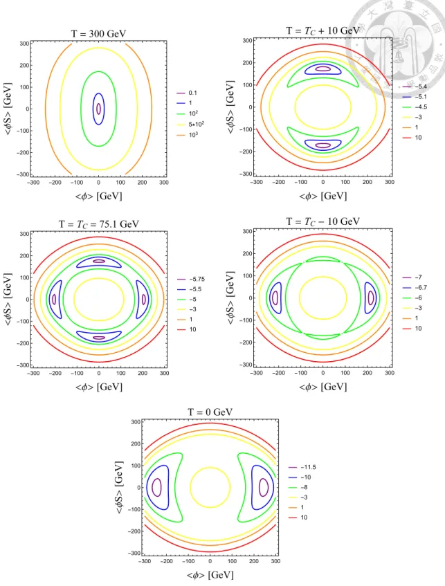
3.1 The contour plots of the HT effective potential in the plane of ⟨ϕ⟩ and

⟨ϕS⟩ at T = 300 GeV (Upper Left), T = TC + 10 GeV (Upper Right), T = T_C = 75.1 GeV (Middle Left), T = T_C−10 GeV (Middle Right) and T = 0 GeV (Lower). The parameters are, m_S = m_H/2 and λ_HS = 0.4.

Note that all the plot legends are in the unit of 10⁷ GeV. . . 21

3.2 The effect of thermal (TGB off, red dot-dashed), non-thermal gauge (GB off, green dashed) and NG bosons (NG off, yellow dotted) contributions on T_C (Left panel) and v_C/T_C (Right panel) in the OS-like scheme. The blue solid line includes all the contributions. . . 22

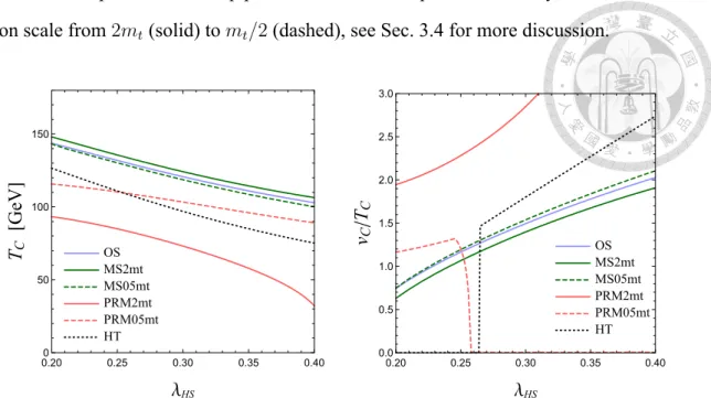
3.3 Comparison of scheme-depended results and investigation of scale depen- dence. Left: Critical temperature as the function of λ_HS. Right: v_C/T_C as the function of λ_HS. The OS-like scheme with NG resummation and the HT scheme are depicted as the blue solid and black dotted lines, respectively. For the MS and the PRM schemes, the style of lines are green and red, respectively. In the legend, “MS2mt (MS05mt)” represents that the MS scheme’s renormalization scale is at 2m_t(m_t/2). Same notation is also applied to the PRM scheme. . . 23

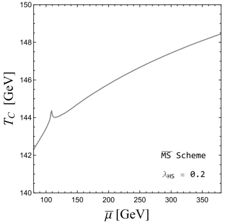
3.4 Critical temperature as the function of renomalization scale in the MS scheme. The parameter settings are λ_HS = 0.2 and m_S = m_H/2. The spike around 109 GeV is expected to be an accidental cancellation among contributions of different particle contents, not any physical or theoretical interest. . . 25

(9)

List of Tables

3.1 The input parameters in all schemes. Note that, besides the MS scheme (see Sec. 2.2), µ_H, µ_S, and λ_H satisfy the tree-level relations: µ²_H = m²_H/2, µ²_S =−m²S+ λ_HS/2v₀²and λ_H = m²_H/2v₀². . . . 18 3.2 Summary of the scheme settings. . . 19 3.3 The percentage of the effects on the EWPT by turning off specific channel. 22

(10)

Chapter 1 Introduction

Cosmic baryon asymmetry (BA) problem [1, 2] is a long-standing and ongoing topic in particle physics and cosmology. Electroweak baryogenesis (EWBG), one of the most promising mechanisms to solve BA, requires a strong first-order electroweak phase transition (EWPT) which creates electroweak(EW)-symmetry-breaking bubble. CP-violating interactions occur at the bubble wall and induce a net density of left-handed fermions. This process makes EW sphalerons produce unequal amounts of baryons and anti-baryons. For a successful EWBG theory, the baryon-number-changing processes have to sufficiently suppress inside the expanding EW-breaking bubbles in order to prevent the wash out. The criterion for above is^*

critial vacuum expectation value, v_c

critical temperature, T_C > ζ_sph(T_C), (1.1) where ζ_sph(T_C) depends on the sphaleron configuration (or topology) [3] and the ﬂuctu- ation determinant [4], etc. The current model [5] has showed that ζ_sph(T_C) ≃ 1.1 − 1.2, where the one-loop effective potential with thermal resummation is used to evaluate the sphaleron energy. However, EWBG cannot be achieved by the standard model (SM) alone, since the discovered Higgs boson with 125 GeV [6] is incompatible to the mech- anism required. To be more specifically, in the SM, the first-order EWPT cannot take

*The critical phenomenology occurs when the potential energy of minima are degenerated and the tun- nelling process happens, i.e. ,the first-order phase transition from EW-symmetry vacuum to EW-breaking vacuum takes place.

(11)

place; instead, the EWPT is a smooth crossover [7]. Further, baryon number will be erasured due to the sphaleron processes. By extending the scalar sector with an SU(2)_L singlet scalar(S), this simplest extension can provide a viable parameter space that makes the first-order EWPT possible. Furthermore, S can also be a dark matter (DM) candidate by imposing a Z₂symmetry [8, 9].

In principle, every physical observable should be independent of any artificial effect.

For exanple, the full Higgs potential should be a gauge-independent quantity. Neverthe- less, in pratice, one has to truncate the calculation at a certian level since the full exact an- alytical form of potential cannot be obtained (in other words, full-loop calculation cannot be achieved). Perturbative effective potential is widely used to analyse EWPT; especially, one- or two-loop expansions are often adopted for various analyses. However, it is well known that any result from this method is depended on the gauge fixing parameter (ξ) [10]. For instance, the Higgs vacuum expectation value (VEV) is varying as one changes ξ. Furthermore, this gauge-dependent issue will contaminate the calculation of baryon- number preservation criterion, Eq. (1.1). As a result, any phenomenological claim and consequence is inherited this ξ dependence. Therefore, the gauge effect should be regu- larized. To be note that one of the exceptions is when the EWPT is driven by the scalar thermal loops or the tree-level barrier where the ξ dependence can be neglected. How- ever, in the singlet extended Abelian-Higgs model, as [11] found that the ξ dependence cannot be ignore even when the presence of the tree-level barrier. This issue is seldom investigated deeply in the context of studying EWPT by SM plus real singlet model.

Apart from the artifical gauge problem, another issue in the effective potential calculations is the occurrence of infrared (IR) divergences. The Higgs mass is obtained from the second derivative of the effective potential. If one adopts a renormalization scheme that one-loop level potentials do not affect the tree-level mass relation, the second derivatives of the Nambu-Goldstone (NG) bosons one-loop potential are ill-defined when ξ in the R_ξ gauge is set as zero. Thus, the Higgs mass is IR divergent in this case. One prescription to resolve is to inculde higher order terms into the NG boson masses [12, 13], i.e., resumming the NG boson masses. In the later, we will show that after the NG masses are resummed,

(12)

their contributions to the Higgs mass are relatively minor compared with other effects.

Nevertheless, their numerical effects on v_C/T_C are unexplored.

In this thesis, the EWPT is revisited in the context of the SM with a real singlet scalar.

To unfold the gauge problem aforementioned, we first analyse the degree of effect on v_C/T_C by subtracting both thermal and non-thermal gauge boson contributions from the effective potential. Even though the exact ξ dependence in the potential cannot be shown in this simple analysis, one can demonstrate numerically the importance of gauge channels in the successful first-order EWPT (vC/T_C ≥ 1), as the ξ dependence mainly comes from the gauge contributions. This method stands as a criterion for whether the investigation of ξ dependence is necessary. Meanwhile, the numerical impact on the NG resummation in the on-shell(OS)-like scheme^†is also analysed.

To avoid the scheme dependence issue, three commonly adopted schemes in the lit- erature are also investigated: (1) the MS scheme, (2) the high-temperature (HT) scheme and (3) the Patel-Ramsey-Musolf (PRM) scheme [4]. In the first scheme, unlike the OS- like scheme, the tree-level NG boson masses are non-zero, since the tree-level relations have been modified because of different tadpole conditions; thus, the aforementioned NG resummations are not required. The potential of the second scheme is defined as: the tree-level potential plus the scalar thermal mass terms only. Obviously, the potential is gauge-independent, because the thermal masses are free of the ξ dependence. In the last scheme, the Nielsen-Fukuda-Kugo (NFK) identity [15, 16] is adopted to obtain the gauge- invariant TC; vC is evaluated at the HT potential at TC in order to keep gauge-invariant.

In the last scheme, taking different potentials to obtain TC and vC may seem inconsistent.

However, this treatment grantees the results are strictly gauge-invariant. Note that the numerical comparison between the PRM scheme and the other gauge-dependent schemes has not performed yet, this is one of our goals to complement this work.

The effective potential is the major ingredient of analyzing EWPT and spontaneous symmetry breaking. For completeness, we briefly introduce the derivation of the effective potential from the partition functional (see [17]) by using the Feynman path integral

†In [14], this scheme is called the on-shell scheme. Because this is not the genuine on-shell renormalization, we call this scheme the on-shell-like scheme instead.

(13)

method [18]. The effective potential in a more specific terminology should be called the generating functional for zero-momentum one-particle irreducible (1PI) Green function.

To begin with, we first recall W [J ],

Z[J] = e^{iW [J ]} (1.2)

which is the generating functional for connected Green’s functions (the detail of generating functional of connecting Green function is shown in Appendix A). Expressing the partition functional,Z[J], with an external source field, J(x), in the path integral representation, we have

Z[J] =N

∫

Dϕ eⁱ^∫^d⁴^x[L(ϕ)+J(x)ϕ(x)] =⟨0⁺|0⁻⟩, (1.3) where N⁻¹ =

∫

Dϕ eⁱ^∫^d⁴^x[^L(ϕ)]. (1.4)

The second equality of Eq. (1.3) is a reminder that the partition function represents a state starts with a no particle state at +∞ position and end with a no particle state at −∞

position. The VEV of ϕ in the presence of J can be defined by

ϕ_c(y) = δW [J ] δJ (y) =

∫ Dϕ ϕ(y) exp( i∫

d⁴x [L(ϕ) + J(x)ϕ(x)])

∫ Dϕ exp( i∫

d⁴x [L(ϕ) + J(x)ϕ(x)]) ,

=⟨0⁺|ϕ(y)|0⁻⟩J,

(1.5)

the last equality shows that ϕ_cis actually a classical field. The physical VEV is

φ(y) = δW [J ] δJ (y)

J =0

= N

∫

Dϕ ϕ(y)eⁱ^∫^d⁴^x[^L(ϕ)] =⟨0⁺|ϕ(y)|0⁻⟩. (1.6)

Furthermore, if we assume that the vacuum has a translational symmetry, the VEV does not depend on the spacetime position any more, i.e.,

ϕ =⟨0|ϕ(x)|0⟩ = ⟨0|e^{iP x}¹ϕ(0)e^{−iP x}²|0⟩ = ⟨0|ϕ(0)|0⟩ = constant field. (1.7)

Motivated by the idea that finding a generating functional provides 1PI connect Green

(14)

function, the effective action provides the exact role. The effective action is defined as a Legendre transformation of W [J ],

Γ[ϕ_c] = W [J ]−

∫

d⁴x ϕ_c(x)J (x),

=−i {

lnN

∫

Dϕ exp [

i

∫

d⁴x (L(ϕ) + J(x)ϕ(x)) ]}

− i {

ln exp [

(−i)

∫

d⁴x J (x)ϕc(x) ]}

,

=−i {

lnN

∫

Dϕ exp [

i

∫

d⁴x (L(ϕ) + J(x) (ϕ(x) − ϕc(x))) ]}

.

(1.8)

In addition,

δΓ[ϕ_c]

δϕ_c(x) = J [x], (1.9)

which can be proved straight forward. The advantage of effective function can be under- stood from the following: while the source field is turning off, ϕ_cthat satisfies Eq. (1.9) is the lowest energy configuration of the theory. This solution has particularly interest in the spontaneous symmetry breaking analysis. The same idea is also applied to the effective potential which will be demonstrated in the later. By shifting the field, ϕ^′ = ϕ−ϕc(the po- sition index is omitted hereafter), and using the definition of action: S(ϕ) =∫

d⁴xL(ϕ), Eq. (1.8) becomes

Γ[ϕ_c] =−ilnN

∫

Dϕ^′ exp {

i [

S(ϕ_c+ ϕ^′) +

∫

d⁴xJ ϕ^′ ]}

. (1.10)

The small shifting of the field can be approximated by expanding the action around the classical field (ϕc),

S[ϕ_c+ ϕ^′] = S[ϕ_c] +

∫

d⁴x δS[ϕ_c+ ϕ^′] δϕ

ϕ^′=0

ϕ^′ + 1

2

∫

d⁴xd⁴y ϕ^′(x)δ²S[ϕ_c+ ϕ^′] δϕ(x)ϕ(y)

ϕ^′=0

ϕ^′(y) +· · · .

(1.11)

(15)

The action satisfies the variational principle; hence δS[ϕ_c+ ϕ^′]

δϕ

ϕ^′=0 = δS[ϕ_c]

δϕ_c = 0, δ²S[ϕ_c+ ϕ^′] δϕ(x)δϕ(y)

ϕ^′=0 = δ²S[ϕ_c] δϕ_c(x)δϕ_c(y),

= iG⁻¹(x, y; ϕ_c),

(1.12)

where G is the two-point Green function. Then Eq. (1.11) can be arranged into

S[ϕc+ ϕ^′] = S[ϕc] + 0 + 1 2

∫

d⁴xd⁴y ϕ(x)iG⁻¹(x, y; ϕc)ϕ(y) +· · · . (1.13)

Because S[ϕ_c] is independent of ϕ, one can bring it out of the integral; then the effective action becomes

Γ[ϕc] = S[ϕc]− ilnN

∫

Dϕ^′ exp {1

2

∫

d⁴d⁴y ϕ(x)G⁻¹(x, y; ϕc)ϕ(y) }

+· · · . (1.14)

The second term can be evaluated by utilizing the equality,

∫ _∞

−∞

d⃗p e⁻¹²^⃗^p^†^A⃗^p+⃗^I^†^⃗^p =

√(2π)ⁿ

detAe¹²^⃗Î^†Â⃗Î, (1.15)

where n is the d.o.f. of p. In our case, ⃗I = 0 and A = iG⁻¹. After absorbing√

(2π)ⁿand N into Dϕ^′, the effective action is

Γ[ϕc] = S[ϕc] + i

2lnDet iG⁻¹(x, y; ϕc) +· · · , (1.16)

= S[ϕ_c] + i

2Trln iGˆ ⁻¹(x, y; ϕ_c) +· · · , (1.17)

= S[ϕ_c] + i 2Trln

∫

d⁴xd⁴y δ(x− y)iG⁻¹(x, y; ϕ_c) +· · · , (1.18)

where the operator Det acts on the spacetime, (x, y) and also any internal space, e.g., color space or spinor space, etc. An identity is used: DetA = exp( ˆTrlnA), where ˆTr acts on the same space(s) as Det. Additionally, if the operator A is a function of spacetime, the functional trace has the property: TrA =∫

d⁴xA(x, x) which is adopted in Eq. (1.18).

We can simplify the above further by performing the integral and expressing the Green

(16)

function in the momentum space, which is convenient for the later use,

Γ[ϕ_c] = S[ϕ_c] + i 2Trln

∫

d⁴x iG⁻¹(x, x; ϕ_c) +· · · , (1.19)

=

∫

d⁴xL(ϕc) + i 2

∫ d⁴p

(2π)⁴Trln iG⁻¹(p; ϕ_c)

∫

d⁴x +· · · , (1.20)

=−V0(ϕ_c)

∫

d⁴x + i 2

∫ d⁴p

(2π)⁴Trln iG⁻¹(p; ϕ_c)

∫

d⁴x +· · · , (1.21)

where we have assumed that ϕ_c is a constant field, so that kinetic term is absent. Since the tree-level potential is independent of spacetime, it can be brought out of the integral.

Finally, the effective potential is defined as the following:

Γ[ϕ_c]≡ −Veff(ϕ_c)

∫

d⁴x, (1.22)

Veff(ϕc) = V0(ϕc)− i 2

∫ d⁴p

(2π)⁴Trln iG⁻¹(p; ϕc) +· · · , (1.23) V1(ϕc) =−i

2

∫ d⁴p

(2π)⁴Trln iG⁻¹(p; ϕc), (1.24)

where V₁ stands for the general one-loop potential of different particle contents. We can now easily understand what the name of effective potential represents: besides the dom- inant tree-level potential, the effective potential represents the potential that includes all the higher order corrections. In our analysis, we require the level of correction isO(¯h) which corresponds to the one-loop level. The detail of derivation of the one-loop level potential for each particle species can be seen in the Appendix B.

The thesis is organized as the following: In Chap. 2, we introduce our model, renormlization schemes and tadpole conditions in each scheme. In addition, the pattern of the EWPT and the method of searching T_C and v_C is outlined. Chap. 3 demonstrates our nu- merical analyses and we discuss the renormalization-scale dependence on T_C. In the end, we discuss the DM issue in the Sec. 4.1; our results are summarized in the Sec. 4.2.

(17)

Chapter 2 Model: SM + Real Singlet Scalar

We consider a model in which SU(2)_Lreal singlet scalar S is added to the SM. S can be the dark matter candidate by imposing the Z₂ symmetry on the Lagrangian [9] (i.e., it is invariant under S → −S). We require S can only couple to the Higgs sector (the higgs portal). The tree-level Higgs potential of the theory is the following:

V₀(H, S) =−µ²HH^†H + λ_H(H^†H)⁴− µ²_S

2 S²+ λS

4 S⁴+λHS

2 H^†HS², (2.1)

where H is the usual complex Higgs doublet. It is written in terms of the components as

H(x) =



 G⁺(x)

√1

2[ϕ + h(x) + iG⁰(x)]



 , (2.2)

where ϕ which will eventually develop the non-zero VEV at≃ 246 GeV represents the constant background field (translational symmetry) of H. The real part of the neutral component of H is h(x), the 125 GeV Higgs boson. G^0,^±(x) stand for the NG bosons.

The superscripts refer to the electric charge of the fields. Presenting the potential in terms

(18)

of components, we have

V₀ = −µ²H

2

{(ϕ + h)²+[

2G⁺G⁻+ (G⁰)²]}

+λ_H 4

{

(ϕ + h)⁴+ 2(ϕ + h)²[

2G⁻G⁺+ (G⁰)²] +[

2G⁻G⁺+ (G⁰)²]2}

−µ²_H

2 S²+λ_S

4 S⁴+ λ_HS 2 S²{

(ϕ + h)²+[

2G⁺G⁻+ (G⁰)²]}

.

(2.3)

The tree-level effective potential can also be represented by using only the constant background fields (denoting background field of S as ϕ_S), by turning off quantum fields (h and G^0,^±),

V₀(ϕ, ϕ_S) = −µ²_H

2 ϕ²+λ_H

4 ϕ⁴−µ²_S

2 ϕ²_S+ λ_S

4 ϕ⁴_S +λ_HS

4 ϕ²ϕ²_S. (2.4)

In order to bound the potential from below, λ_H and λ_S must be greater than zero. In addition, another condition is necessary if λHS < 0. In the region that both ϕ and ϕSare large, we can denote ϕ_S = ϕδ, where δ is a number. The relevant terms in the potential become

V₀ ∼ 1

4(λ_H + λ_Sδ⁴ + λ_HSδ²)ϕ⁴. (2.5) To keep the bracket always greater than zero for arbitrary δ, we require

λ²_HS < 4λHλS, if λHS < 0. (2.6)

Note that a local minimum in the S direction will appear as µ²_S > 0. The EW-broken vacuum should be the global minimum in the present universe: V₀(v, 0) < V₀(0, v^sym_S ), where the superscript means that the singlets VEV is in a EW-symmetry phase. This condition requires that

−µ²H

2 v²+λ_H

4 v⁴ < −µ²S

2 (v_S^sym)²+ λ_S

4 (v_S^sym)⁴. (2.7)

By the minimum conditions at the tree level, v_S^sym = √

µ²_S/λ_S and µ²_H = λ_Hv², we can

(19)

rearrange above into

λ_S > λ_Hµ⁴_S

µ⁴_H ≡ λ^minS . (2.8)

In the numerical analyses, we took λ_S = λ^min_S + 0.1. This choice makes first-order phase transition possible and it is also adopted in [14]. Tadpole conditions are scheme- dependent. The general form is

T_h(S)≡

⟨∂V_eff

∂ϕ_(S)

⟩

= 0, (2.9)

where⟨· · ·⟩ denotes that the term inside the bracket is evaluated in a vacuum and all quan- tum fields are taken as zero. The order of level of the effective potential (tree or loop, etc.) is evaluated depends on the corresponding scheme. The Landau gauge (ξ = 0) is taken when evaluating the gauge contributions, except the PRM scheme.

2.1 On-shell-like Scheme (OS-like)

The OS-like scheme requires that the loop corrections hold the tree-level relations when the one-loop corrections are added. Therefore, the renormalization conditions are^*

⟨∂(V_CW+ V_CT)

∂ϕ

⟩

= 0,

⟨∂²(V_CW+ V_CT)

∂ϕ²

⟩

= 0,

⟨∂²(V_CW+ V_CT)

∂ϕ²_S

⟩

= 0, (2.10)

where V_CT are the counter terms, and V_CW is the Coleman-Weinberg potential [19]:

VCT =−δµ²_H

2 ϕ²− δµ²_S

2 ϕ²_S, (2.11)

V_CW(m²_i) = ∑

i

n_i m⁴_i 4(16π²)

( logm²_i

µ² − ci

)

, (2.12)

which is regularized in the MS scheme (see Appendix B). m_irepresents different background- field-dependent masses (see the Appendix D for detail); its subscript stands for a particle’s species. We include the Higgs bosons (H_1,2, eigenstates of the scalar sector), NG bosons

*Note that checking the first derivative of the one-loop potential with respect ϕSis trivial, since the Z2

symmetry guarantees it is zero.

(20)

(G^±, G⁰), the gauge bosons (W, Z) and top quark (t). The degree of freedom (d.o.f.) and its statistic of the particle is denoted as n_i: n_H_1,2_,G⁰ = 1, n_G± = 2, n_Z = 3, n_W = 6 and n_t=−12. For the scalars and the top quark, c = 3/2, and for the gauge bosons, c = 5/6.

µ represents the renormalization scale.

The tadpole conditions for the OS-like scheme at the tree level are

Th ≡

⟨∂V₀

∂ϕ

⟩

= v (

−µ²H + λHv²+λ_HS 2 v_S²

)

= 0, (2.13)

TS ≡

⟨∂V₀

∂ϕ_S

⟩

= vS

(

−µ²S+ λSv²_S+λ_HS 2 v²

)

= 0, (2.14)

where v and v_Sare the VEVs of the doublet Higgs and S, respectively. For the Z₂-invariant EW-broken vacuum (ϕ = v₀, ϕ_S = 0), µ²_H = λ_Hv²₀ and v_S^Br = 0. Therefore, the Higgs boson masses in the vacuum are

m²_H =

⟨∂²V₀

∂ϕ²

⟩

=−µ²H + 3λ_Hv₀², (2.15) m²_S =

⟨∂²V0

∂ϕ²_S

⟩

=−µ²S+λHS

2 v₀². (2.16)

NG Resummation

If we use Eq. (2.12) to evaluate the second condition of Eq. (2.10), one can notice that while mi equals to zero, which is the case for the NG bosons at the electroweak vacuum, a IR divergent term appears: λ²_Hϕ²(log m²_G/µ²)|ϕ→v0; regardless of what the value of µ is.

However, the existence of a IR problem often indicates that a theory is incomplete. In this case, it shows that the necessity of including the higher order correction to the NG boson masses, i.e., we need to resum the NG boson contributions. We adapt the same procedure as [12, 13], m_G → MG = m_G+ Σ_G, where Σ_G is the one-loop self-energy of the NG

(21)

boson with the vanishing external momenta:

Σ_G= 1 16π²

[

3λ_Hm²_H₁ (

log m²_H₁ µ² − 1

) + 1

2λ_HSm²_H₂ (

logm²_H₂ µ² − 1

)

+3g₂² 2 m²_W

(

logm²_W µ² −1

3 )

+3(g₂²+ g²₁) 4 m²_Z

(

log m²_Z µ² − 1

3 )

− 6yt²m²_t (

logm²_t

µ² − 1)]

,

(2.17)

where g₁ and g₂ are the gauge couplings of U(1) and SU(2)_L, respectively, and y_tis the top Yukawa coupling. To solve δµ²_H, δµ²_S and µ numerically, we need to m_G → MGin the NG boson channels of Eq. (2.12), and combine the CT terms (Eq. 2.11); finally, solve the renormlization conditions Eq (2.10), simultaneously.

2.2 MS Scheme

In the MS scheme, the tree-level relations are modified when the higher-order corrections are added in. In the other words, Eq. (2.15) and Eq. (2.16) will be modified by one-loop level contributions. We impose the tadpole conditions on the one-loop level,

T_h ≡

⟨∂(V₀+ V₁)

∂ϕ

⟩

= v (

−µ²H + λ_Hv²+λ_HS 2 v²_S

) +

⟨∂V_CW

∂ϕ

⟩

= 0, (2.18) T_S ≡

⟨∂(V₀+ V₁)

∂ϕ_S

⟩

= v_S (

−µ²S+ λ_Sv_S² +λ_HS 2 v²

) +

⟨∂V_CW

∂ϕ_S

⟩

= 0, (2.19)

by using the same solution like above (ϕ = v₀, ϕ_S = 0); as a result, we have relations

µ²_H = λHv²₀ + 1 v₀

⟨∂V_CW

∂ϕ

⟩

, (2.20)

⟨∂VCW

∂ϕ_S

⟩

= 0. (2.21)

(22)

The Higgs masses are

m²_H =

⟨∂²(V₀+ V₁)

∂ϕ²

⟩

= (

−µ²_H + 3λ_Hv²+ λ_HS 2 v²_S

) +

⟨∂²V_CW

∂ϕ²

⟩

, (2.22) m²_S =

⟨∂²(V₀+ V₁)

∂ϕ²_S

⟩

= (

−µ²S+ 3λ_Sv²_S+λ_HS 2 v²

) +

⟨∂²V_CW

∂ϕ²_S

⟩

. (2.23)

Rearranging above by inputting the solution (ϕ = v₀, ϕ_S = 0) and using Eq. (2.20), we have

m²_H = 2λ_Hv²₀− 1 v₀

⟨∂V_CW

∂ϕ

⟩ +

⟨∂²V_CW

∂ϕ²

⟩

, (2.24)

m²_S =−µ²S+λHS

2 v₀²+

⟨∂²VCW

∂ϕ²_S

⟩

. (2.25)

We can solve µ_S, µ_H and λ_H through Eq. (2.24), Eq. (2.25) and Eq. (2.18), numerically.^† Note that we set the renormalization scale of Eq. (2.12) at the range from 2m_t ∼ 0.5mt. Since the NG boson masses are non-zero at the electroweak-broken vacuum, we do not need resummation as the OS-like scheme.

2.3 Thermal History and Thermal Potential

Like [20] pointed out that a two-step phase transition pattern increases the accessibility of EWBG. The pattern of two-step phase transition we are interested in is the following:

the global vacuum of the early hot universe was (ϕ, ϕ_S) = (0, 0). While the universe was cooling down, a primary phase transition (PT) occurred, the global minimum are transited to singlet direction (S) at (0, v_SC), an EW-symmetry-preserving minimum. As the universe approached a critical temperature (T_C) where the potential energy of doublet (H) and singlet minima are degenerate, the global vacuum tunnelled (required to be a first-order PT) to an EW symmetry-breaking minimum (v_C, 0). At the present universe whose temperature is approximately zero, the vacuum arrived at (v0 ≃ 246 GeV, 0).

To investigate above scenario, the dynamic of thermal potential is essential for study-

†In Eq. (2.24), actually, the basis of the scalar sector for calculating VCWdoes not limit to the mass eigenstates; h, S basis is also available, due to the absence of hhS coupling. On the other hand, in Eq. (2.25), one must use mass eigenstates because of the existence SSh coupling.

(23)

ing the evolution of the universe. In the OS-like, the MS and the PRM (Sec. 2.5) schemes, we use the finite-temperature one-loop effective potential given by [21]:

V₁^T(ϕ, ϕ_S, T ) = ∑

i

n_i T⁴ 2π²I_B,F

(m²_i T²

) ,

where I_B,F(a²) =

∫ _∞

0

dx x²ln (

1∓ e⁻^√^x²^+a²) .

(2.26)

In the numerical computation, we use the approximated functions (see Appendix C) for computational efficiency. In addition, since the perturbative expansion is invalid when temperature is high, the thermal potential needs to be resummed. We replace m²_i with thermally corrected masses,

m²_i −→ m²i + Σ_i(ϕ, ϕ_S, T ), (2.27)

where Σ_i(ϕ, ϕ_S, T ) are the thermal masses (a more refined resummation method can be refered to, e.g., [22]), the exact forms can be found in the Appendix D. Notice that although thermal resummation is performed in the OS-like and the MS schemes, it is not performed in the PRM scheme; since we consider onlyO(¯h) = 1 in the PRM scheme (see Sec. 2.5 for detail) and the thermal resummation isO(¯h) = 2 effect.

2.3.1 Standard method of searching T

_C

and critical VEVs

For a successful two-step EWPT, v_C, T_C, v_SC^Br and v_SC^symare found numerically through the following equations and satisfying the inequalities:

V_eff(ϕ = v_C, ϕ_S = v^Br_SC, T_C) = V_eff(ϕ = 0, ϕ_S = v_SC^sym, T_C), (2.28)

∂V_eff

∂ϕ

vC, vBr_SC, TC

= ∂V_eff

∂ϕ_S

0, vsym

SC , TC

= 0, (2.29)

∂²V_eff

∂ϕ²_(S)

vC, vBr_SC, TC (0, vsym

SC , TC) > 0, (2.30)

(24)

det

∂²V_eff/∂ϕ² ∂²V_eff/∂ϕ∂ϕ_S

∂²V_eff/∂ϕ_S∂ϕ ∂²V_eff/∂ϕ²_S

vC, vBr_SC, TC (0, vsym

SC , TC)

> 0, (2.31)

where the last two inequalities assure that the minima are not saddle points. In Sec.2.5, we will discuss that why the standard method of determining T_C and VEVs depends on the choice of gauge.

2.4 High Temperature (HT)

Both the OS-like and the MS schemes have gauge-dependent potential at the one-loop level. The high temperature approximation scheme provides a gauge-free and efficient method to investigate EWPT. This scheme simply includes the tree-level potential and the Higgs thermal mass terms which are taken from high temperature approximation at the O(2) of Eq. (C.1.1):

V^HT(ϕ, ϕ_S, T ) = V₀(ϕ, ϕ_S) + 1

2Σ_H(T )ϕ²+ 1

2Σ_S(T )ϕ²_S, (2.32)

where ΣH and ΣS are the Higgs thermal masses which are gauge-independent [23], see Eq. (D.5, D.6) for detail. Because this scheme is gauge-free and ignores all the other loop contributions, we can obtain the gauge-invariant T_C and VEVs from this potential in relatively efficient way compared with previous schemes. In the PRM scheme (Sec. 2.5), we also use this potential to evaluate VEVs.

2.5 Patel-Ramsey-Musolf (PRM) Scheme

The main goal of the PRM scheme is to get gauge-free results. Unlike the HT scheme, the PRM scheme takes the one-loop order corrections and the thermal effects into account. As the tadpole conditions are set at the tree level, the tree-level conditions are preserved. The renormalization scale is set same as the MS scheme which is varied from 2m_t ∼ 0.5mt. In the next subsection, we elaborate how the PRM scheme utilizes NFK identity to get gauge-free results.

(25)

2.5.1 Gauge-independent T

_C

and VEVs

The NFK identity [15, 16] tells us that^‡

∂Veff(ϕ, ξ)

∂ξ =−C(ϕ, ξ)∂Veff(ϕ, ξ)

∂ϕ , (2.33)

where C(ϕ, ξ) is a functional. In fact, T_Ccan be proved formally to be gauge-independent with the identity and Eq. (2.28)[4] as long as we are working on the full order of the effec- tive potential. However, in the practical calculation for T_C, one could only calculate the potential up to some order. For example, like in our previous standard method of deter- mining T_C includes only the one-loop order effect; thus, this causes an artificial violation of the NFK identify, even though the full order formalism is gauge-invariant. In order to regulate this issue, we have to keep tracking whether the identity is valid in each order of

¯

h. In the perturbation theory, in principle, we can expand V_effand C in the power of ¯h:

V_eff(ϕ) = V₀(ϕ) + ¯hV₁(ϕ, ξ) + ¯h²V₂(ϕ, ξ) +· · · , (2.34) C(ϕ, ξ) = c₀+ ¯hc₁(ϕ, ξ) + ¯h²c₂(ϕ, ξ) +· · · . (2.35)

By inserting them into Eq. (2.33), we get

¯

h∂V₁(ϕ, ξ)

∂ξ + ¯h²∂²V₂(ϕ, ξ)

∂ξ² +· · · = − c0

∂V₀

∂ϕ − ¯h (

c₁(ϕ, ξ)∂V₀(ϕ)

∂ϕ + c₀∂V1(ϕ, ξ)

∂ϕ )

+O(¯h²) +· · · ,

(2.36)

where we had expressed Eq. (2.33) in ¯h order. Since the tree-level potential is free of ξ-dependence, c0 = 0. AtO(¯h),

∂V₁(ϕ, ξ)

∂ξ = c₁(ϕ, ξ)∂V₀(ϕ)

∂ϕ . (2.37)

‡Even though our potential is a two dimensional (ϕ, ϕS) function, the procedure is straight forward: by taking the other dimensions as zero, one can get a pair of Eq. (2.33). Using the same method described in above, one can get similar results.

(26)

Eq. (2.37) shows that as long as we are working onO(¯h), the gauge dependence of V1(ϕ, ξ) is vanished at stationary point(s) of the tree-level potential. On the contrary, T_Cand VEVs determined by the standard method are evaluated in the tree-level plus one-loop potential minima; as a result, those results are gauge-dependent. Extending above to our model, the ξ dependence of V₁(ϕ, ϕ_S, ξ) disappears while we evaluate T_C at the tree-level minima:

(ϕ = v^tree = 246 GeV, ϕ_S = 0) and (ϕ = 0, ϕ_S = v^tree_S = √

µ²_S/λ_S). For the two-step EWPT, the gauge-independent T_C can be obtained from the following:

V₀(v^tree, 0) + V_CW(v^tree, 0) + V₁^T(v^tree, 0, T_C)

= V₀(0, v_S^tree) + V_CW(0, v_S^tree) + V₁^T(0, v_S^tree, T_C).

(2.38)

Note that as we are working onO(¯h), the thermal resummation, a two-loop order O(¯h²) effect, is not performed. Going beyondO(¯h) requires two-loop contributions which is out of scope of our current analysis. In the Appendix E, we give an example to explicitly show how the gauge dependence disappears when the potential is evaluated at the tree- level minima.

The minima, v_C and v_SC, are inherited gauge dependence which can easily be un- derstood from the NFK identity: in Eq. (2.33), the field value minimizing the effective potential is gauge-dependent. To get gauge invariant VEVs in the PRM scheme, we have to utilize the HT potential, Eq. (2.32), by finding the minima at T_C, i.e., find the minima of V^HT(ϕ, ϕ_S, T_C).

(27)

Chapter 3 Numerical Analysis

In our model, mS, λS and λHS are the free parameters. We take mS = mH/2 which is within DM experiment bound and phenomenology (see Sec. ?? for the discussion), and choose λ_S = λ^min_S + 0.1, see Eq. (2.8); thus only λ_HS is varied in the analyses. Aiming to investigate the gauge dependence, a range of λ_HS is selected where the tree-level potential is relatively minor compared with gauge loop contributions to the potential barrier.

Furthermore, this particular range meets the conditions of the two-step strong first-order EWPT (v_C/T_C ≃ 1 and several inequalities in Sec. 2.3.1). For clarity, our input param- eters are listed in Table 3.1, and we summarize the settings of the each scheme in Table 3.2.

In Sec. 3.1, we list a detail procedure of finding T_Cand v_C; in addition, their precisions in the analyses are also shown. Our analyses can be divided into two parts: Sec. 3.2 focuses on the effect of gauge and the NG boson channels in the OS-like scheme, Sec. 3.3 demonstrates how the scheme dependence influences the results.

Parameter

m_H v₀ m_W m_Z m_t Value [GeV] 125 246 80.4 91.1 173.2

Table 3.1: The input parameters in all schemes. Note that, besides the MS scheme (see Sec. 2.2), µ_H, µ_S, and λ_H satisfy the tree-level relations: µ²_H = m²_H/2, µ²_S = −m²S + λ_HS/2v₀² and λ_H = m²_H/2v₀².

(28)

Scheme

OS-like MS HT PRM

Tadpole Condition Tree 1-loop Tree Tree

NG resummed √

- - -

Thermal resummed √ √

- -

ξ dependence √ √

- -

Table 3.2: Summary of the scheme settings.

3.1 Critical Temperature and Critical VEV

Two s of method of finding T_C are used; For the PRM scheme, T_C is found by Eq. 2.38.

For the OS-like, the HT and the PRM schemes, T_C is searched by the bisection method whose details of procedure are listed in the following^*:

1. choose two initialized temperatures, T_max(e.g., 200 GeV) and T_min(100 GeV). To use the bisection method, one also needs a middle value, T_mid = (T_max+ T_min)/2 (150 GeV),

2. calculate the energy difference, ∆E, between the potential energy of minima in singlet’s, E(ϕ^min), and doublet’s, E(ϕ^min_S ), directions^†at T_mid, i.e.,

∆E(T_mid) = E(ϕ^min, T_mid)− E(ϕ^minS , T_mid), (3.1)

3. calculate ∆E at T_min, that is

∆E(T_min) = E(ϕ^min, T_min)− E(ϕ^minS , T_min), (3.2)

4. if ∆E(T_mid)× ∆E(Tmin) < 0, we can redefine T_min → Tmin, and T_max → Tmid, otherwise T_min→ Tmidand T_max→ Tmax,

5. take the new Tmidand Tminback to the step 2. and go though the procedure again.

The above is calculated iteratively until

*We useMathematica to analyse our model.

†We use theFindminimum, the optional methods InteriorPoint and PrincipleAxis are chose.

標準模型之實數純量擴展:電弱相變之規範與方策依賴探討

國立臺灣大學理學院物理學所 碩士論文

Graduate Institute of Physics College of Science

National Taiwan University Master Thesis

標準模型之實數純量擴展:

電弱相變之規範與方策依賴探討

Standard Model with a Real Singlet Scalar: An Investigation of Scheme Dependence and Gauge

Dependence in Electroweak Phase Transition

李彥頲 Yen-Ting Li

指導教授：蔣正偉 博士

Advisor: Cheng-Wei Chiang, Ph.D.

中華民國 107 年 11 月

November, 2018

誌謝

Acknowledgements

摘要

Abstract

Contents

List of Figures

List of Tables

Chapter 1 Introduction

Chapter 2

Model: SM + Real Singlet Scalar

2.1 On-shell-like Scheme (OS-like)

2.2 MS Scheme

2.3 Thermal History and Thermal Potential

2.3.1 Standard method of searching T

and critical VEVs

2.4 High Temperature (HT)

2.5 Patel-Ramsey-Musolf (PRM) Scheme

2.5.1 Gauge-independent T

and VEVs

Chapter 3

Numerical Analysis

3.1 Critical Temperature and Critical VEV

國立臺灣大學理學院物理學所碩士論文

指導教授：蔣正偉博士