國立臺灣大學理學院心理學研究所 博士論文
Graduate Institute of Psychology College of Science
National Taiwan University Doctoral Dissertation
色彩在對稱知覺各階層的角色
The Role of Color in Symmetry Detection – from Local to Global
吳佳瑾 Chia-Ching Wu
指導教授:陳建中 博士 Advisor: Chien-Chung Chen, Ph.D.
中華民國 100 年 6 月
June, 2011
i
致謝
2008 年春,是我博士班生涯的一個重要轉捩點。當時,我從原來高等思考 推理的領域轉進了陳建中老師的視知覺實驗室。這三年來,在陳老師的帶領與 指導下,我得以一窺視知覺這個領域的奧妙,也深深感受到身為一個優秀研究 者所需要的學識、涵養、熱忱與責任。這篇論文的完成,首先要感謝、也最要 感謝的,也是我的指導教授陳建中老師。
其次要感謝的是所有的口試委員--黃榮村校長、黃淑麗老師、孫慶文老師
、簡惠玲老師、姜自強老師、與葉素玲老師。幾位老師在論文計劃口試和學位 論文口試時都給了我相當寶貴的意見,他們思考的深度與廣度、以及對做學問 的態度,每每讓我在短短兩個小時的口試中獲益良多。
再來,我也要特別感謝我的三位受試者,願意花這麼多時間參與實驗,因 為有他們的全力配合,實驗才得以順利進行。此外,也感謝所有視覺實驗室的 成員們一路上的陪伴和幫忙,以及冠嫺助教總是親切且有條不紊地為我們這些 研究生處理相關的行政事務,讓我們可以無後顧之憂,專心在學業上。
最後,我要感謝的是在漫長博士班生涯中陪伴我、支持我的家人和朋友。
謝謝我的父母無條件的支持,一路走來只有鼓勵和信任,而沒有給我任何壓力
。也謝謝所有關心我、陪伴我、支持我的朋友們:有著堅定革命情感的緯倫、
純慧、蓓蓓;同在學術路上互相扶持互相砥勵的蔚倫、幸釗、延叡、婷文、慧 雅;以及我最最親愛的好友們:士凱、寶哥、阿恕、小外、毓倫、奕晴、小珊
、曉萍、曦羽、惠棠、阿鍾…等。也許隨著時空的遷移,我們已分散在不同的 城市不同的國家,但那些共同的回憶卻永遠深藏在我心中。
ii
iii
中文摘要
對稱是一高階的視覺特徵,其辨識須仰賴人類視覺系統的複雜運算。在自 然情境中,對稱圖形或物體通常伴隨著多種顏色,因此視覺系統必須整合顏色 和形狀的訊息才能偵測到彩色的對稱圖形。本研究以五個實驗來探討顏色在對 稱知覺中所扮演的角色。我們將對稱偵測機制分為兩階段—配對與統合,並分 別檢驗此兩階段是否對顏色有選擇性反應。研究結果顯示此兩階段均對顏色有 選擇性的反應,此表示視覺系統中有一組對顏色選擇性反應的對稱偵測系統。
我們進一步操弄了影像中所包含的顏色數目,來探討視覺系統如何整合這些對 稱偵測系統來偵測彩色對稱。研究結果顯示無論觀察者是否知道對稱圖案的對 稱軸方向,一影像中顏色數目的增加都可以促進對稱偵測的表現。我們也比較 了當兩不同顏色對稱圖形共享相同的對稱軸與否時的對稱偵測表現,以探討是 否不同顏色能區隔兩圖形而促進對稱的偵測。研究結果顯示,當兩圖形共享一 對稱軸時,其對稱的偵測會比兩圖形的對稱軸方向不同時要佳。我們提出一整 合了線性的對稱偵測機制、非線性的反應模式、反應干擾的特性與多個系統的 決策歷程的彩色對稱偵測模型來解釋以上的結果。此模型顯示一影像中顏色數 目的增加會減少對稱偵測系統中的抑制作用,進一步促進對稱偵稱的表現。此 外,當兩對稱圖形共享同一對稱軸時,兩對稱偵測系統間的抑制作用會減少,
而導致其對稱偵測表現較兩圖形的對稱軸有不同方向的對稱軸時來得佳。
關鍵詞:對稱偵測、高階色彩視覺、顏色與形狀的整合、心理物理學、雜訊遮 蔽。
iv
v
The Role of Color in Symmetry Detection – from Local to Global
Chia-Ching Wu
Abstract
Symmetry is a higher-order form that requires a complicated computation in the visual system. In a nature scene, symmetric objects or stimuli may come with any combination of color. Hence, human visual system needs to integrate both color and form information to detect chromatic symmetry. In this study, we conducted five experiments to investigate the role of color in symmetry detection. We distinguished two stages, that is, matching and pooling stage, of the symmetry encoder and examined the color selectivity of these two stages of symmetry encoder. Our results showed that these two stages are color-selective. This suggests that there are a band of color-selective symmetry channels in our visual system. We further manipulated the number of the colors in the images to investigate how human visual system integrates the response of these symmetry channels to detect chromatic symmetry. Our results showed that the increment of the number of the colors facilitated the symmetry detection performance, regardless the observers had prior knowledge of the symmetry axis orientation or not. Finally, we examined the symmetry detection in two images sharing the same axis or not, to see whether the segmentation of two images with different colors helps symmetry detection. The results however showed better symmetry detection performance when two symmetric patterns shared the same axis
vi
than those did not. All these results can be accounted for by a computational model that incorporated linear symmetry encoding mechanisms, nonlinear transducer response, noise manipulation and a multiple channel based decision making process.
The model fitting results suggests that the increment of the number of the color reduces the inhibition of the symmetry channels, and in turn facilitates the symmetry detection performance when the images contain more than one color. In addition, the inhibition between channels responding to the two symmetric patterns sharing the same axis is smaller than that between channels responding to two patterns in different axes, in turn facilitates the symmetry detection performance when the two images shared the same symmetry axis.
Keywords: symmetry detection, higher-order color vision, color and form integration, psychophysics, noise masking.
vii
Contents
致謝 ... i
中文摘要 ... iii
Abstract ... v
Contents ... vii
List of Tables ... ix
List of Figures ... xi
Chapter 1 Introduction ... 1
1.1. Higher-Order Color Processing ... 2
1.2. Mechanism of Symmetry Detection ... 5
1.3. Chromatic Symmetry Detection ... 8
1.4. Overview of this Thesis ... 10
Chapter 2 2AFC Noise Masking Paradigm ... 13
Chapter 3 Chromatic Symmetry Detection Model ... 17
Chapter 4 General Method ... 23
4.1. Equipment ... 23
4.2. Specification of the Chromatic Content of the Stimuli ... 23
4.3. Stimuli ... 26
Chapter 5 Color-Selective Matching Stage ... 29
5.1. Method ... 35
5.2. Results ... 37
5.3. Discussion ... 41
Chapter 6 Color-Selective Pooling Stage ... 45
6.1. Method ... 47
viii
6.2. Results ... 48
6.3. Discussion ... 52
Chapter 7 Integration of the Color-Selective Symmetry Channels ... 57
7.1. Method ... 59
7.2. Results ... 61
7.3. Discussion ... 67
Chapter 8 Color Facilitation in Symmetry Detection under Uncertainty of Axis Orientation ... 75
8.1. Method ... 75
8.2. Results ... 76
8.3. Discussion ... 85
Chapter 9 The Integration of Color-Selective Symmetry Detection Channels within the Same and between the Different Axes ... 95
9.1. Method ... 96
9.2. Results ... 97
9.3. Discussion ... 104
Chapter 10 General Discussion ... 111
10.1. Color Selective in the Higher-Order Form Mechanism ... 113
10.2. Integrative Color-Form Processing ... 114
10.3. Independent Luminance and Chromatic Processing ... 116
10.4. Contributions and Limitations ... 117
10.5. Future Directions ... 120
Reference ... 123
Appendix Contrast Detection Threshold Measurement of the Selected Color ... 137
Curriculum Vitae ... 139
ix
List of Tables
Table 4.1. The coordinates of the color space and chromoluminance cone contrast
space of the color. ... 26
Table 7.1. Fitted model parameters. ... 71
Table 8.1. Fitted model parameters. ... 89
Table 9.1. Fitted model parameters. ... 108
x
xi
List of Figures
Figure 1.1. Diagram of the model. See text for details.
... 7Figure 1.2. Diagram of the chromatic symmetry detection model. See text for details.
.... 9
Figure 1.3. The components of chromatic symmetry detection model Chapter 5 to 9
involves. See text for details. ... 10
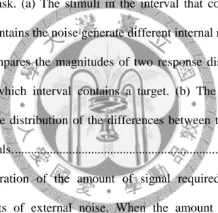
Figure 2.1. The internal representation in a two-alternative forced-choice (2AFC)
noise masking task. (a) The stimuli in the interval that contains the target and noise and that contains the noise generate different internal response distributions.
An observer compares the magnitudes of two response distributions to make a decision about which interval contains a target. (b) The internal response of comparison is the distribution of the differences between the internal responses to the two intervals. ... 14
Figure 2.2. An illustration of the amount of signal required to detect target at
different amounts of external noise. When the amount of external noise is relatively small, the increase of the external noise does not influence the amount of signal required. When the amount of external noise is much larger than that of internal noise, the amount of signal required increases with the increment of the external noise. The transition point (Neq) of these two regimes reveals the magnitude of the internal noise of the system. ... 15
Figure 4.1. Cone contrast color space. The grid corresponds to the isoluminant plane,
which includes the Red/Green (0° – 180°) and Blue/Yellow (90° – 270°) cardinal mechanisms axes. The vertical axis is the achromatic axis (-90° – +90°). ... 25
xii
Figure 5.1. Three possible ways the symmetry encoder acts in the matching stage. (a)
The symmetry encoder only pairs the image features of the same color. (b) The symmetry encoder can pair the image features of the opponent colors. (c) The symmetry encoder is not color-selective. It pairs the corresponding image features regardless their colors. ... 30
Figure 5.2. The stimulus composed of achromatic large image elements. Panel a and
b were symmetry and anti-symmetry respectively. (From Mancini et al., 2005) 31
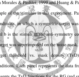
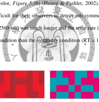
Figure 5.3. The stimuli Pashler and his colleges used. Panel a is a 2-color symmetric
display. Panel b is an anti-symmetric display. Both are the examples of symmetry. (From Morales & Pashler, 1999 and Huang & Pashler, 2002.) ... 32
Figure 5.4. The example of the stimulus in this experiment. Panel a is the stimuli in
the symmetry conditions, in which a symmetric target was superimposed on the noise mask. Panel b is the stimuli in the anti-symmetry conditions, in which an anti-symmetric target was superimposed on the noise mask. ... 37
Figure 5.5. The target threshold vs. mask density (TvD) functions for four
isoluminance conditions. Each panel represents the data from one observer. The left column represents the TvD functions for the RG (red symbols) and the Anti- RG (blue symbols) conditions. The right column represents the TvD functions for the RB (pink symbols) and the Anti-RB (green symbols) conditions. ... 38
Figure 5.6. The target threshold vs. mask density (TvD) functions for four luminance
conditions. Each panel represents the data from one observer. The left column represents the TvD functions for the WK (red symbols) and the Anti-WK (blue symbols) conditions. The right column represents the TvD functions for the WR (pink symbols) and the Anti-WR (green symbols) conditions. ... 40
Figure 5.7. The average threshold elevation at different noise densities in four anti-
xiii
symmetry conditions compared with their corresponding symmetry conditions.
The open symbols represent the threshold elevation in luminance conditions (pink up-triangles and green down-triangles for the Anti-WK and the Anti-WR respectively). The filled symbols represent the threshold elevation in isoluminance conditions (red circles and blue squares for the Anti-RG and the Anti-RB respectively). ... 41
Figure 6.1. Three possible ways the symmetry encoder acts in the pooling stage. (a)
The symmetry encoder only counts the pairs of the same color for the computation of the symmetry axis. (b) The symmetry encoder counts the pairs as signal as long as their colors are from the same color opponent channels. (c) The symmetry encoder is not color-selective. All the pairs are taken into account to determine the symmetry axis regardless of their colors. ... 46
Figure 6.2. The example of the stimuli: (a) the red target superimposed on the noise
mask of its own color (0° deviation) and (b) the red target superimposed on the noise mask of green color (180° deviation). The mask density was 1%. ... 48
Figure 6.3. The results of isoluminance conditions. Each panel represents data from
one observer. The red and blue symbols denote the target density thresholds for red and blue target superimposed on the noise mask of various colors respectively. The pink and cyan symbols denote the red and blue target density threshold when there was no mask, serving as a baseline. ... 49
Figure 6.4. The results of luminance conditions. Each panel represents data from one
observer. The black symbols denote the target density thresholds for white target superimposed on the noise mask of various colors. The gray symbol denotes the target density threshold when where was no mask, serving as a baseline. ... 51
Figure 6.5. The target stimuli of control experiment. Each target image was
xiv
composed of two symmetric patterns of same or different colors. (a) Image A was a red right-diagonal symmetric pattern superimposed on a red left-diagonal symmetric pattern. (b) Image B was a red left-diagonal symmetric pattern superimposed on a green right-diagonal symmetric pattern. ... 54
Figure 7.1. The example of the stimuli. Panel a, b, and c represent the target of 1, 2,
and 4 colors superimposed on the noise mask of the same colors as the target respectively. ... 60
Figure 7.2. Target threshold vs. mask density (TvD) functions for the isoluminance
conditions. Each panel represents the data from one observer. The red, blue, green, purple, and pink symbols represent the data points of the R, B, RG, RB, and RGBY conditions respectively. The smooth curves are fits of the model (see text for details). ... 62
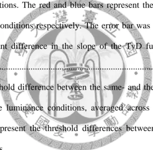
Figure 7.3. The average slopes of the target threshold vs. mask density (TvD)
functions for the 1- (red bar), 2- (blue bar) and 4-color isoluminance conditions (green bar) at low noise densities respectively. The error bar represents the stand error. There is significant difference in the slope of the TvD function between the 1- and 2-color conditions and between the 1- and 4-color conditions. ... 63
Figure 7.4. The average threshold change produced by the two 2-color (RG and RB,
green and blue symbols) and the one 4-color (RGBY, orange symbols) isoluminance conditions at different noise densities. The error bar was the standard error. ... 63
Figure 7.5. Target threshold vs. mask density (TvD) functions for the luminance
conditions. Each panel represents the data from one observer. The red, green, purple, and pink symbols represent the data points of the W, WK, WR, and WKRG conditions respectively. The smooth curves are fits of the model (see text
xv
for details). ... 65
Figure 7.6. The average slopes of the target threshold vs. mask density (TvD)
functions for the 1- (red bar), 2- (blue bar) and 4-color luminance conditions (green bar) at low to median densities. The error bar was the stand error. There was significant difference in the slope of the TvD functions between the 1- and 2-color conditions and between the 1- and 4-color conditions. ... 66
Figure 7.7. The average threshold change produced by the two 2-color (WK and WR,
gray and pink symbols) and the one 4-color (WKRG, brown symbols) condition at different noise densities. The error bar was the standard error. ... 66
Figure 7.8. The amount of the parameter Si
b.tc in five isoluminance and fourluminance conditions. The red, blue, green, purple, and orange symbols represent the value of Sib.tc in the R, B, RG, RB, and RGBY condition respectively. The gray, black, pink, and brown symbols represent the value of Sib.tc in the W, WK, WR, and WKRG condition respectively. The light-red and dark-gray dotted lines represent the average of Sib.tc in the 1-, 2-, and 4-color isoluminance and luminance conditions respectively. ... 72
Figure 7.9. The amount of the parameter z' in the 1-, 2-, and 4-color conditions for
each observer. The red, blue, and green symbols represent the value of the parameter z’ for observer CCW, CPY, and HYC respectively. The amount of the parameter z' for each observer decreases with the increment of the number of the colors in the images. ... 73
Figure 7.10. The number of the possible candidates each noise dot can pair with
decreases when the number of the colors increases. The yellow dashed ovals in Panel a and b represent the possible pairs a red noise dot x’ can form in the 1- and 4-color images respectively. The red noise dot x’ can pair with all the dots in
xvi
the image in the panel a while can only pair with two dots in the panel b. ... 74
Figure 8.1. Target threshold vs. mask density (TvD) functions for three isoluminance
conditions. Each panel represents the data from one observer. The red, green and blue symbols represent the data points of the 1- (R), 2- (RG), and 4-color (RGBY) conditions respectively. The smooth curves are fits of the model (see text for details). ... 77
Figure 8.2. The average threshold change produced by the increment of the number of
the colors at different noise densities in the isoluminance conditions. The green and purple symbols represent the threshold difference between the 2-color (RG) and the 1-color (R) conditions and between the 4-color (RGBY) and the 1-color (R) conditions respectively. ... 79
Figure 8.3. Target threshold vs. mask density (TvD) functions for luminance
conditions. Each panel represents the data from one observer. The gray and brown symbols represent the data points of the 1- (W) and the 2-color (WK) condition respectively. The smooth curves are fits of the model (see text for details). ... 80
Figure 8.4. The average threshold change between the 2-color (WK) and the 1-color
(W) luminance conditions. The error bar represents the standard error. ... 81
Figure 8.5. Target threshold vs. mask density (TvD) functions for the 1-color
isoluminance (R) and luminance (W) conditions. Each panel represents the data from one observer. The red and gray symbols represent the data points of the R and W condition respectively. The smooth curves are fits of the model. ... 82
Figure 8.6. Target threshold vs. mask density (TvD) functions for the 2-color
isoluminance (RG) and luminance (WK) conditions. Each panel represents the data from one observer. The green and brown symbols represent the data points
xvii
of the RG and WK conditions respectively. The smooth curves are fits of the model. ... 83
Figure 8.7. The average threshold difference in the target density threshold between
isoluminance and luminance conditions. The red and blue symbols represent the threshold difference between the 1-color (R vs. W) isoluminance and luminance conditions and between the 2-color (RG vs. WK) isoluminance and luminance conditions respectively. ... 84
Figure 8.8. The amount of the parameter Si
t.tc in the isoluminance and luminanceconditions. The red symbols represent the amount of Sit.tc in the 1- (R), 2- (RG), and 4-color (RGBY) isoluminance conditions. The gray symbols represent the amount of Sit.tc in the 1- (W) and 2-color (WK) luminance conditions. ... 91
Figure 8.9. The number of the possible candidates each dot in the symmetric pattern
can pair with decreases when the number of the colors increases. The yellow dashed ovals in Panel a and b represent the possible pairs a red dot x’ can form in the 1- and 4-color symmetric images respectively. The dot x’ can pair with all the dots in the image in the panel a while can pair with only one dot in the panel b. 93
Figure 9.1. Target threshold vs. mask density (TvD) functions in the isoluminance
condition. Each panel represents the data from one observer. The red and green symbols represent the data points of the RG-S and RG-D conditions respectively.
The smooth curves are fits of the model (see text for details). ... 98
Figure 9.2. Slope of the target threshold vs. mask density (TvD) functions in
isoluminance conditions. The red and blue bars represent the slopes of the RG-S and the RG-D conditions respectively. The error bar was standard error. There was no significant difference in the slopes of the TvD functions between two conditions. ... 99
xviii
Figure 9.3. The threshold difference between the same- and the different-orientation
conditions in the isoluminance conditions, averaged across three observers. The red symbols represent the threshold difference between the RG-S and the RG-D conditions. ... 100
Figure 9.4. Target threshold vs. mask density (TvD) functions in the luminance
conditions. Each panel represents the data from one observer. The gray and brown symbols represent the data points of the WK-S and the WK-D conditions respectively. The smooth curves are fits of the model (see text for details). ... 101
Figure 9.5. Slope of the target threshold vs. mask density (TvD) functions in
luminance conditions. The red and blue bars represent the slopes of the WK-S and the WK-D conditions respectively. The error bar was standard error. There was no significant difference in the slope of the TvD functions between two conditions. ... 102
Figure 9.6. The threshold difference between the same- and the different-orientation
conditions in the luminance conditions, averaged across three observers. The gray symbols represent the threshold differences between the WK-S and the WK-D conditions. ... 102
Figure 9.7. The threshold difference between two same-orientation and between two
different-orientation conditions, averaged across three observers. The pink symbols represent the threshold difference between the RG-S and the WK-S conditions. The green symbols represent the threshold difference between the RG-D and the WK-D conditions. ... 103
1
Chapter 1 Introduction
Mirror symmetry (henceforth, symmetry) is one of the principal organizational factors in the perceptual grouping of discrete objects (Koffa, 1935; Köhler, 1929;
Wertheimer, 1938) that can facilitate figure ground segmentation, object recognition and shape representation (e.g., Blum, 1973; Burbeck & Pizer, 1995; Driver, Baylis, &
Rafal, 1992; Kovacs, Feher, & Julesz, 1998; Leeuwenberg & Buffart, 1984; Marr, 1982). Since human visual system can detect symmetry as quickly as in less than 100 ms, symmetry detection is regarded as an intrinsic, fundamental process of the human visual system (e.g., Barlow & Reeves, 1979; Carmody, Nodine, & Locher, 1977;
Hogben, Julesz, & Ross, 1976; Julesz, 1971; Locher & Nodine, 1989; Wagemans, Van Gool, & d’Ydewalle, 1991; Wagemans, Van Gool, Swinnen, & Van Horebeek, 1993). Several simple spatial features in the image are important to symmetry perception, such as contrast, spatial frequency, edge, and the orientation of symmetry axis. However, few researches investigated the role of color in symmetry detection (Huang & Pashler, 2002; Morales & Pashler, 1999; Troscianko, 1987). Actually, since color vision and spatial vision are considered as two different disciplines in vision research, there are few studies on space-color interactions in the higher-order visual process in general.
Symmetry is a higher-order image feature that requires a complicated information processing and computation in the visual system (Chen & Tyler, 2010;
Tyler & Hardage, 1996). If a symmetric image contains more than one color, human visual system has to integrate both spatial and chromatic information to form chromatic symmetry perception. Hence, investigating the role of the color in
2
symmetry perception helps us to understand both the mechanisms for higher-order color vision and the mechanisms for complex forms. In this thesis, we used a noise masking paradigm and a computational model to achieve these goals:
(1) To examine how the symmetry channel integrates color information.
(2) To characterize the properties of the color-selective symmetry channel.
(3) To investigate how multiple color-selective symmetry channels interact with each other.
1.1. Higher-Order Color Processing
The extraction of color information in the visual system starts with the spectrum selective response of three different types of retinal photoreceptors, i.e., long- (L), middle- (M), short- (S) wavelength selective cones on the retina (e.g., Bowmaker &
Dartnall, 1980; Jacobs & Neitz, 1993; Schnapf, Kraft, & Baylor, 1987; Smith &
Pokorny, 1975; van Kries, 1905; Vos & Walraven, 1971). Each cone type absorbs different spectrums of light. Their spectrum selective responses are then sent to the striate visual cortex (V1) through the retinogeniculate pathways. The spectral sensitivities of the retinogeniculate cells are largely consistent with three independent color opponent channels measured with psychophysic methods (for a review, see Knoblauch & Shevell, 2004). The V1 neurons receive inputs from the retinogeniculate pathways and have their fibers project to the extrastriate cortex (V2, V3, and V4) and the inferotemporal (IT) cortex through the ventral pathway (for a review, see Gegenfurther & Kiper, 2004). More than 50% cells in these areas selectively respond to color (Dow & Gouras, 1973; Gegenfurtner, Kiper, &
Fenstemaker, 1996; Gegenfurtner, Kiper, & Levitt, 1997; Gouras, 1974; Johnson, Hawken, & Shapley, 2001; Komatsu & Ideura, 1993; Komatsu, Ideura, Kaji, &
3
Yamane, 1992; Schein & Desimone, 1990; Thorell, De Valois, & Albrecht, 1984;
Yates, 1974; Zeki, 1973).
The ventral pathway also processes information about the identity of a visual object, such as the form or shape. Thus, it is possible that the processing of color and that of form are contingent in the visual system. It has been shown that almost all cells in V1 are orientation selective while about 50% cells in V1 are color-selective (Dow
& Gouras, 1973; Gouras, 1974; Johnson et al., 2001; Thorell et al., 1984; Yates, 1974). While there are non-color selective neurons respond only to lines or edges in an image regardless their color, many V1 cells can simultaneously encode both the chromatic and spatial characteristics, such as orientation, of a stimulus (Johnson et al., 2001; Leventhal, Thompson, Liu, Zhou, & Ault, 1995). A number of studies identified different organizations of receptive filed of them, such as the double- opponent cells in which the spatial-opponency and the color-opponency coincide exactly, to investigate the color processing in such a spatial information selective mechanism (Livingstone & Hubel, 1984; Michael, 1978a, 1978b, 1978c, 1979; Ts’o
& Gilbert, 1988). The psychophysical studies also showed the visual system encodes both chromatic and spatial information with a property similar to that of V1 neurons (Chen, Foley, & Brainard, 2000; Switkes, Bradley, & De Valois, 1988; Webster, De Valois, & Switkes, 1990).
Further downstream, the encoding of color tuning in the higher order visual cortex is not clear. It is shown that neurons in V2 and V4 have distinct color selectivity. However, they may tune to any color on the isoluminance plane rather than just the four cardinal directions (Levitt, Kiper, & Movshon, 1994). To probe the higher order color vision mechanisms, one approach is to study the color processing in complex forms. For instance, some studies used Glass pattern, which contains
4
randomly distributed dot pairs whose orientations are determined by certain geometric transforms (Glass, 1969; Glass & Perez, 1973), to investigate the color mechanism in the global form processing (Cardinal & Kiper, 2003; Mandeli & Kiper, 2005;
Rentzeperis & Kiper, 2010; Wilson & Switkes, 2005). The Glass Pattern detection mechanism contains two stages: a local stage and a global stage. The local stage is considered an early visual processing. It uses linear filters to extract information about pair orientation information. The global stage is a higher-order visual processing. It pools the local orientation information across pairs to exact the global structure (Cardinal & Kiper, 2003; Chen, 2009; Mandeli & Kiper, 2005; Smith, Bair, &
Movshon, 2002; Wilson & Switkes, 2005; Wilson, Switkes, & Valois, 2004; Wilson
& Wilkinson, 1998). While the previous research agreed that the local stage is color- selective (Mandeli & Kiper, 2005; Wilson & Switkes, 2005), the color selectivity of the global stage is controversial. Wilson and Swikes (2005) suggested that the global stage is mediated by a non color-selective mechanism while Cardinal and Kiper (2003) suggested that Glass patterns are detected by a multitude of mechanisms that sum their inputs linearly. How the global form mechanism integrates the local information to yield a global form percept is unclear. In this thesis, we investigated the role of the color in symmetry detection in order to understand the higher-order color and pattern vision. The benefit of using symmetric patterns is that the symmetry computation, unlike in Glass patterns where the local grouping plays an important role, always requires long-range interactions and thus provides a better picture of long-range color processing.
5
1.2. Mechanism of Symmetry Detection
Symmetry is a higher-order image feature. A visual stimulus is symmetric if some part of this stimulus is a reflection of another part about an axis, called symmetry axis. To determine whether an image is symmetric, the observer has to compare whether two points of the image are identical, and, if yes, whether the middle points of these matches forms an axis. Such operation requires a higher-order visual mechanism to take the information from early stage into computation.
Currently, in the literature, two types of theories have been proposed to explain how the visual system achieves this task. The first, the relational structure theory, suggests that the visual system may simply analyze the spatial relationship among individual image elements and determine an image to be symmetric if the relative position of a sufficient proportion of image elements supports it. That is, symmetry detection would be based solely on the signal-to-noise ratio or “weight of evidence”
in the image (Csathó, van der Vloed, & van der Helm, 2004; van der Helm &
Leeuwenberg, 1996, 1999). The second, the spatial filtering theory, assumes that a band of linear filters, whose sensitivity profiles contain multiple excitatory and inhibitory regions, extract symmetry information from an image. (Dakin & Hess, 1997; Dakin & Watt, 1994; Gurnsey, Herbert, & Kenemy, 1998; Osorio, 1996;
Rainville & Kingdom, 1999, 2000, 2002; Scognamillo, Rhodes, Morrone, & Burr, 2003; Tjan & Liu, 2005). These filters may be oriented (Dakin & Watt, 1994;
Rainville & Kingdom, 2000) or have different phase sensitivity (Rainville &
Kingdom, 1999, 2000, 2002; Scognamillo et al., 2003). These filters operate on the input images. If an input image is symmetric, the filtered image would contain features at or across the symmetry axis that can be picked up by a second-order filter that has an orientation similar to that of the symmetry axis (Gurnsey et al., 1998;
6
Scognamillo et al., 2003) or by a simple mathematical operator operating orthogonal to the symmetry axis (Dakin & Hess, 1997; Dakin & Watt, 1994; Rainville &
Kingdom, 1999, 2000, 2002).
Both theories propose a two-stage processing for symmetrical perception. For the relational structure theory, the symmetry detection mechanism has to decide which image elements have the spatial properties that are consistent with a symmetric pair (signal) and which are not (noise). Then a higher-order mechanism collects these local pairs to compute the overall signal-to-noise ratio. The spatial filtering theory also needs a higher-order filter to monitor the output of lower order linear filters, which extracts symmetry information from an image. For these two theories to work, however, one has to make an assumption about the location and orientation of the symmetry axis, on which all the operations on the image depend. However, mirror symmetry can occur at any orientation in a nature scene. While these two theories perform well to explain the data from experiments with a known symmetry axis orientation, their generalization is limited as they do not address the situation where the symmetry axis orientation is unknown to the observers. To solve this problem, Chen and Tyler (2010) manipulated the cueing of the axis orientation and the axis salience and measured the target detection threshold at various noise density levels under these conditions. Their results showed facilitation effect of both cueing of axis orientation and high axis salience. However, the amount of cueing effect and the nonlinear axis salience effect cannot be explained by the above two theories. Hence, they incorporated the property of two-stage encoding process, adding a nonlinear process that was neither addressed by the relational structure nor by the filter approach, to explain the effect of uncertainty about axis orientation in the framework of the Signal Detection Theory (Green & Swets, 1966).
7
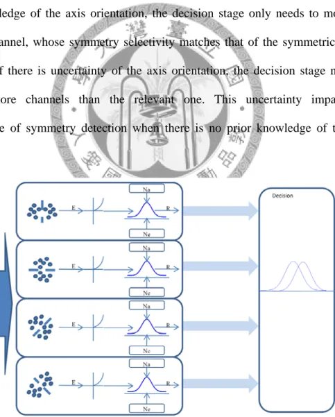
Their model contains two stages: a perception stage and a decision stage (Figure 1.1). In the perception stage, there are a band of orientation-selective symmetry encoders that are sensitive to symmetry in an image. Each encoder is sensitive to the mirror symmetry about one axis. The contribution of each encoder is limited by both the internal noise inherited in the system (Na in Figure 1.1) and the external noise provided by the noise patterns (Ne in Figure 1.1). The nonlinear response of the perception stage is sent to the decision stage. The detection performance relies on the maximum response of all monitored channels. The observers detect symmetry when the difference of responses between two intervals reaches unity. If the observers have prior knowledge of the axis orientation, the decision stage only needs to monitor a relevant channel, whose symmetry selectivity matches that of the symmetric image.
However, if there is uncertainty of the axis orientation, the decision stage needs to monitor more channels than the relevant one. This uncertainty impairs the performance of symmetry detection when there is no prior knowledge of the axis orientation.
Figure 1.1. Diagram of the model. See text for details.
8
This model has an extra nonlinear process than the spatial filtering theory and relational structure theory as these two theories are incapable of explaining Chen and Tyler (2010) data. This model is therefore more powerful than other two approaches.
This model provides us a good theoretical basis for exploring the possible mechanisms underlying color processing in symmetry perception. In this thesis, we extend Chen-Tyler model (2010), taking the chromatic information into consideration, to investigate the mechanism of chromatic symmetry detection.
1.3. Chromatic Symmetry Detection
The symmetric objects or images in the natural scene often contain more than one color. To form a chromatic symmetry percept, human visual system has to integrate both spatial and chromatic information. Previous research showed that the observers can discriminate the yellow symmetrical pattern from random pattern on isoluminant green background (Troscianko, 1987). It suggested that color can support symmetry. The symmetry detection mechanism must be capable of processing color information. However, how visual system integrates both spatial and color information is unclear. In this thesis, we expand Chen-Tyler model (2010) to cover both spatial and color information in symmetry detection.
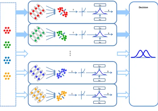
Figure 1.2 illustrates our model for chromatic symmetry detection. There are a
band of symmetry channels sensitive to the symmetry of the image in this model.
Each channel has its symmetry encoder, which is sensitive to the mirror symmetry of a certain color about one axis. The main difference between this model and Chen- Tyler model (2010) is that there are many symmetry encoders each with a different color selectivity. Notice that each symmetry channel tunes to only one color. This is only plotted here only to convey the idea of multiple channels.
9
To recognize chromatic symmetry, the symmetry encoders need to encode chromatic symmetry information first, that is, to decide which color pairs are the signal while other are not. Computationally, each symmetry encoder can be divided into two steps. In the first step, matching, the symmetry encoder has to extract corresponding color features in an image; and then, pooling, the symmetry encoder has to analyze those color pairs to determine whether their equal-distance points form a symmetry axis. In this stage, the pairs of the same color with the equal-distance points about a symmetry axis are regarded as the signal of that orientation axis while other dots are noise. The registered signal excites the symmetry channel selective to that axis and the color of the signal. The visual system needs to integrate the information from these color-selective symmetry channels to form a chromatic percept.
Decision E R
Na
Ne
E R
Na
Ne
R E
Na
Ne
R E
Na
Ne
Figure 1.2. Diagram of the chromatic symmetry detection model. See text for details.
10
1.4. Overview of this Thesis
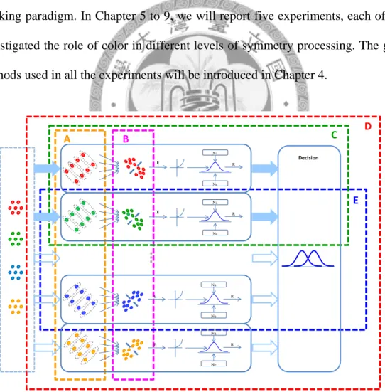
This chromatic symmetry detection model provides us a framework to investigate the color processing in the symmetry detection. We examined the properties of the matching and pooling stages in this thesis, and then investigated how visual system integrates these channels to detect chromatic symmetry. We used a two- alternative forced choice (2AFC) noise masking paradigm to characterize the response properties of the symmetry channels to probe this issue. In Chapter 2, we will introduce the noise masking paradigm used in this thesis. Chapter 3 introduces the details of our chromatic symmetry detection model when it is applied to a 2AFC noise masking paradigm. In Chapter 5 to 9, we will report five experiments, each of which investigated the role of color in different levels of symmetry processing. The general methods used in all the experiments will be introduced in Chapter 4.
Figure 1.3. The components of chromatic symmetry detection model Chapter 5 to 9 involves. See text for details.
A B D
E C
Decision E R
Na
Ne
E R
Na
Ne
R E
Na
Ne
R E
Na
Ne
11
Figure 1.3 illustrates the different components of the model to be investigated by
different chapters. Chapter 5 and 6 concern the color selectivity of symmetry encoders (box A and B in Figure 1.3). In the Chapter 5, we manipulated the colors of the signal pairs in the symmetric patterns as the same or different and compared their detection thresholds, to investigate the color-selective property of the matching stage of the symmetry encoders (box A in Figure 1.3). Chapter 6 concerns the color selectivity of the pooling stage of the symmetry encoders. We measured the target detection thresholds at noises of various colors to examine the existence of the independent symmetry encoders (box B in Figure 1.3). In Chapter 7 to 9, we measured the target detection thresholds at various noise densities to get the target threshold vs. noise density (TvD) functions in different conditions, to reveal the characteristics of different channels and their interaction. Chapter 7 concerns the integration of color- selective symmetry channels selective to the same orientation (box C in Figure 1.3).
We manipulated the number of the colors in the images containing a vertical symmetric pattern to probe this issue. Chapter 8 concerns how visual system integrates the symmetry channels selective to different colors and orientations to detect symmetry when there is uncertainty of axis orientation (box D in Figure 1.3).
We manipulated the number of the colors in the images containing either a left- or right-diagonal symmetric pattern and compared their TvD functions to achieve this goal. In Chapter 9, we compared the characteristics of the integration between two symmetry channels selective to the same axis (box C in Figure 1.3) with two symmetry channels each with different orientation selectivity (box E in Figure 1.3).
We superimposed two symmetric patterns that share the same symmetry axis or have different orientation selectivity on each other and measured their TvD functions to achieve this goal. This can help us to understand through what mechanism our visual
12
system forms one coherent symmetry percept rather than two. Chapter 10 is a general discussion about the above studies. We will discuss the implication, the contribution and the limitation of our studies in this chapter.
13
Chapter 2 2AFC Noise Masking Paradigm
We used a 2AFC noise masking paradigm to measure the target density threshold in all the experiments throughout this project. In a trial of the 2AFC noise masking paradigm, the observer was presented with two intervals, one of which contained a symmetric target (the exception is the experiment in Chapter 9, in which there were two targets superimposed on each other, see method section of Chapter 9 for details) while another one contained a random-dot noise control. Both target and noise control were superimposed on the different amounts of random noise mask. The observer’s task was to judge which interval contained a target.
The noise masking paradigm allows us to measure the detection threshold of different symmetry types at various noise levels and thus provide information that reveals the internal response properties of human observers (for a review, see Lu &
Dosher, 2008). According to Signal Detection Theory (Green & Swets, 1966), the observer’s decisions are based on the probability distributions of internal response to the noise and to the signal plus the noise. (Figure 2.1a). In a 2AFC task, these two distributions are provided by the responses to the two test intervals in a trial. That is, in each trial, the observer compares the magnitudes of the two internal responses and decides which one of the two intervals generates a greater internal response and thus contains the target. Mathematically, this comparison can be achieved by observing whether the response difference to the two intervals to be greater than zero. Thus, our main concern can be placed on the distribution of the difference between the internal responses to the two intervals (Figure 2.1b).
14
The variability of the internal response distributions comes from two sources, the external noise manipulated by the experimenter and the intrinsic noise of the system.
If the external noise is relatively low, the variability of the distribution is dominated by the internal noise. Thus, the performance is not affected by the change in the external noise. A relatively constant amount of signal is required for the observer to detect the target (the dashed horizontal line in Figure 2.2). However, when the external noise is much greater than the internal noise, the variability of the response distribution is determined by the external noise. Increasing the amount of signal is
μ1 μ2
σ1 σ2
Noise Target plus
noise a.
μ 2– μ1
σD
Internal response b.
Figure 2.1. The internal representation in a two-alternative forced-choice (2AFC) noise masking task. (a) The stimuli in the interval that contains the target and noise and that contains the noise generate different internal response distributions. An observer compares the magnitudes of two response distributions to make a decision about which interval contains a target. (b) The internal response of comparison is the distribution of the differences between the internal responses to the two intervals.
15
thus necessary for the observer to detect the symmetry target as external noise increases (the dashed oblique line in Figure 2.2). At the transition point of these two regimes, the amounts of the internal and the external noises are equal (Neq in Figure
2.2).
Hence, by manipulating the amounts of the external noise, we can measure the target detection threshold at different amounts of noise, and in turn the target threshold vs. noise density (TvD) function. The transition point on the TvD function reveals the magnitude of the internal noise of the system. The slope of the TvD function reflects the nonlinear property of the response mechanism. This allows us to estimate the internal response properties of human observers more accurately, to
Figure 2.2. An illustration of the amount of signal required to detect target at different amounts of external noise. When the amount of external noise is relatively small, the increase of the external noise does not influence the amount of signal required. When the amount of external noise is much larger than that of internal noise, the amount of signal required increases with the increment of the external noise. The transition point (Neq) of these two regimes reveals the magnitude of the internal noise of the system.
Neq The amount of external noise
The amount of signal
16
investigate the response properties of symmetry channels. To investigate how human visual system integrates the responses of color-selective symmetry channels in symmetry detection, we manipulated the number of the colors in the stimuli in the 2AFC noise mask task and got their TvD functions. The properties of the TvD functions allow us to investigate the interaction of the channels in different conditions.
The next chapter introduces our chromatic symmetry detection model and how we used it to account for the properties of the TvD functions in the 2AFC noise masking paradigm.
17
Chapter 3 Chromatic Symmetry Detection Model
In this chapter, we introduce our chromatic symmetry detection model and describe how we apply it to the 2AFC noise masking task used in the experiments.
Note that in each trial of the task, the stimuli consisted of either a symmetric target or a non-symmetric random-dot control superimposed on a random-dot mask. All stimuli in a trial contained the same number of the colors with equal probability, in which the number of the color (n) was from 1 to 4.
As Figure 1.2 shown, the chromatic symmetry detection model contains two stages: a perception stage and a decision stage. The perception stage concerns the noise-limited sensitivity of a visual mechanism to the stimuli limited by both internal and external noise, while the decision stage concerns the effect of uncertainty on the decision criterion.
The first step of the perception stage is a band of color-orientation selective symmetry encoders that are sensitive to symmetry in an image. Each encoder is sensitive to the mirror symmetry about one axis with a certain color. As mentioned in Chapter 1, each encoder contains two steps, matching and pooling. The matching stage extracts the corresponding color features in an image while the pooling stage analyzes those color pairs to determine whether their equal-distance points form a symmetry axis. In other words, these symmetry encoders are long-range pairs of local multiplicative color detectors that register a signal whenever there is their target color at two locations in the field equidistant from a symmetry axis. The outputs of all such pairs of detectors relative to a given symmetry axis are linearly summed to form the symmetry signal relative to that location. Only when a number of them line up with
18
respect to a particular symmetry axis, the symmetry encoders regard the chromatic pattern as symmetry.
In the 2AFC noise masking task, the image in the interval that contains target plus mask can be considered to consist of two components: the symmetric target and the noise mask, while the image in the interval that contains noise control plus mask can be considered to consist of just one component with a density that is the sum of the control and the mask.
For a sparse n-color random-dot pattern, the excitation of the j-th color-selective symmetry encoder to the i-th image component, Eji, is
i i j i
j
D
Se n
E
1,
, = ⋅ (1)
where Sej,i is the sensitivity of the j-th symmetry encoder to i-th image component, while 1/n*Di, is the dot density of the pattern of the j-th encoder’ target color in i-th image component. The total excitation of j-th encoder, Ej, is the sum of excitations produced by all image components,
∑
= i ji
j
E
E
, . (2)The response of the perception stage is the excitation of the j-th symmetry encoder, Ej, raised by a power p, and then divided by a divisive inhibition term Ij plus an additive constant z,
19 z
I R E
j p j
j = + (3)
where Ij is the summation of a non-linear combination of the inhibition from all image components to mechanism j. This divisive inhibition term Ij can be represented as
∑
⋅ −
+
⋅
= i
q
i nc
i j q
i tc i j
j D
n Si n
nD Si
I 1 1
. , .
, (4)
where Sij,i.tc and Sij,i.nc are a positive value serving as the inhibition term from the image components consisting of the target color and of the non-target color respectively.
The contribution of each channel to the visual performance is limited by both internal noise of that channel and the external noise provided by the noise patterns.
The variability of the internal noise, σa2
, is a constant for all symmetry channels. The variability of external noise, σe2
, is proportional to the square of the density of random noise mask, that is, σe2
= v * Db2
in which v is a scalar constant and the index b denotes the noise mask. Pooled together, in each channel the standard deviation of the response distribution is
(
b2 a2)
1/2r v D σ
σ = ⋅ + . (5)
The output of the perception stage is then sent to the decision stage. The decision stage monitors more channels than those that are relevant to the visual tasks (Pelli, 1985). The performance of the system is limited not only by the noise in the relevant
20
channels but also by that in the irrelevant channels. In our experiment, the task of the observer was to detect the symmetry component in an image. Hence, a relevant channel is the one whose color-orientation selectivity matches that of the image. The observer detects a symmetric pattern if the maximum response of all monitored channels to an image is greater than the response of a random-dot pattern by an amount that exceeds the level of noise in the system (Green & Swets, 1966).
When there are m channels, in which n channels are relevant while m-n channels are irrelevant, to be monitored, the maximum response of these channels can be described by a distribution whose mean approximates a fourth-power summation over these m channels (Graham, Robson, & Nachmias, 1978; Quick, 1974; Pelli, 1985), though the Gaussian distribution theory of Tyler and Chen (2000) shows that the fourth power exponent is valid only for the restricted conditions of a particular attention model and a linear signal transducer. Hence, for the target plus mask images where there are n channels responding the symmetry image component, the mean of the response R’ can be expressed as
(
1 1 4,( ))
1/44 ) (
' + =
∑
= , + +∑
m= + + nj j b c
n
j j b t
t
b R R
R , (6)
where the subscript b and t denote the noise control pattern and the symmetry component in the images respectively. Instead, the mean of the response R’ for the noise control plus noise mask images is
(
1)
1/44 ) (
'b+c=
∑
mj= Rj,b+cR , (7)
21
in which the subscript b+c indicates that the image contains both the noise mask and a control pattern with the same number of dots as the corresponding symmetry target.
The decision variable, d’, is the difference of the response to the image with the symmetry component and the response to the random-dot control image divided by the standard deviation of the max distribution, σp. That is,
( R
b tR
b c)
pd
'= ' + − ' +σ
(8)The threshold is defined when d’ reaches unity. Note that the standard deviation of the max distribution of multiple independently and identically distributed samples is k times the standard deviation of the original distribution, in which the variable k can be estimated by the method Chen and Tyler (1999) proposed. Thus, σp = σr for 1-color condition while σp = k*σr for n-color conditions.
The above is the description of our chromatic symmetry detection model that applies to a 2AFC noise masking task. In Chapter 5 and 6, we examined the color- selective property of the symmetry encoders in the model. In Chapter 7 to 9, we manipulated the number of the colors in the images and measured the symmetry detection threshold to get the TvD functions, to investigate the integration of these symmetry channels in different conditions. The details of the model implementation are described in each chapter.
22
23
Chapter 4 General Method
In this thesis, our aim is to understand how visual system integrates both color and spatial information to form symmetry perception. To understand how symmetry mechanism processes the color information of the images coming from different color channels, we selected the colors in the stimuli on the MB-DKL color space, in which the chromatic content of color is defined by three cardinal axes based on the response properties of three post-receptoral mechanisms (Derrington, Krauskopf, & Lennie, 1984; Krauskopf, Williams, & Heeley, 1982; MacLeod & Boynton, 1979). This chapter introduces the way we constructed the color space to define the color content of the stimuli and the general method among all the experiments.
4.1. Equipment
All experiments in this study used the same equipment. The visual stimuli were presented on a 24-inch calibrated LCD monitor controlled by a Macintosh computer via a Radeon 7200 graphic board which provided 10-bit digital-to-analog converter depth. The LCD monitor was calibrated with a PhotoResearch PR655 radiometer for both luminance and chromaticity. The viewing distance was set in a way that each pixel extended 2 o visual angles. The refresh rate of the monitor was 60Hz.
4.2. Specification of the Chromatic Content of the Stimuli
In all of the experiments, the display had a mean luminance of 76.81 cd/m2 and mean chromaticity at (0.33, 0.33) in CIE 1931-xy coordinates. All the colors of the display were along a straight line in cone excitation space. The color can be
24
represented by a cone contrast vector (Brainard, 1996) at each point in space. Since the stimuli were composed of 8-th power Gaussian spots, we described their contrast by giving the three cone contrast at the center of the spots. The L-cone contrast, CL, was defined as ∆L/L0 where L0 was the L-cone excitation produced by the background and ∆L =L - L0 was the L-cone excitation deviation at the central point of the spots. If there was a decrement in cone excitation at the central point, the cone contrast was negative. The M-cone and S-cone contrasts, CM and CS, were defined similarly and each color was given by the column vector C = [CL, CM, CS]T. Cone excitations and contrasts were calculated using the Stockman-Sharpe estimates of the cone spectral sensitivities (Stockman & Sharpe, 2000). For calculations, each sensitivity was normalized to a maximum of one and spectra were expressed in units of watts/(sr – m2 - nm). The LMS cone excitation vector of background was [6.056 5.235 2.701]T.
We specified all the colors in term of their contrast and chromoluminance direction. Chromoluminace direction was given by the normalized vector, C /∥C∥, where the notation ∥C∥denoted the length of the vector C. The contrast of each color was defined as c = (CL2
+ CM2
+ CS2
)0.5/(3)0.5. This measure was proportional to the square-root of cone contrast energy and varies between 0 and 1. Contrast was expressed in dB re 1 which equaled 20 log10 c. The contrast of each color in all the experiments was set at its three fold threshold for each observer, based on a subjective sensitivity experiment (see Appendix for details).
Except for some colors in the experiment of Chapter 6, all the colors of the stimuli were in the cardinal directions of the color space (Derrington et al., 1984;
Krauskoph et al., 1982; MacLeod & Baynton, 1979). As shown in Figure 4.1, the black and white were in the luminance direction (-90° – +90°), of which the L, M, S cone contrasts is [0.577, 0.577, 0.577]. The red, green, blue, and yellow were in the
25
Red/Green (0°–180°) and Blue/Yellow (90°–270°) isoluminant directions whose cone contrasts were [0.416, -0.909, 0] and [0, 0, 1] respectively. The nominal isoluminant directions were orthogonal to the CIE2007 luminous efficiency function Vλ (CIE, 2007), which corresponded to the normalized column vector [0.853, 0.522, 0]T in the cone contrast space.
For the convenience of discussion, we used descriptive color names rather than cone contrasts for the modulation directions to describe the colors in our stimuli.
Table 4.1 lists the descriptive color names of the colors we used, their coordinates in the DKL color space and in the cone contrast space.
Figure 4.1. Cone contrast color space. The grid corresponds to the isoluminant plane, which includes the Red/Green (0° – 180°) and Blue/Yellow (90° – 270°) cardinal mechanisms axes. The vertical axis is the achromatic axis (-90° – +90°).
Luminance
Blue/Yellow
Red/Green
26
Name Coordinates in DKL space Coordinates in the cone contrast space (CL, CM, CS)
White (W) (0°, 90°) [0.577, 0.577, 0.577]
Black (K) (0°, -90°) [-0.577, -0.577, -0.577]
Red (R) (0°, 0°) [0.416, -0.909, 0.000]
Blue (B) (90°, 0°) [0.000, 0.000, 1.000]
Green (G) (180°, 0°) [-0.416, 0.909, 0.000]
Yellow (Y) (270°, 0°) [0.000, 0.000, -1.000]
4.3. Stimuli
All stimuli were chromoluminance images composed of the dots distributed in an invisible grid, excluding some checks at the center region and near axis (see method section in each chapter). The width of each check was 7 pixels, corresponding to 0.21o visual angle. The display had a 9.9o visual angle extent in the experiments of Chapter 5 to 7 while a 12.1o visual angle extent in the experiments of Chapter 8 and 9. Each dot was defined by a 8-th power Gaussian function, or K(x, y) = BG + BG.* C exp(x8/2σ8 + y8/2σ8) where x and y were the distances in degrees from the fixation point, σ = 0.11o was the space constant; BG was a 3 by 1 vector that specified the cone excitation coordinates of the background; C was the 3 by 1 cone contrast that specified the color modulation respectively, and the symbol .* denoted element by element multiplication of two vectors.
The stimuli on each trial consisted of three components: the symmetric target, the non-symmetric random-dot control, and the random-dot mask. Both the control
Table 4.1
The coordinates of the color space and chromoluminance cone contrast space of the color.
27
and the mask were composed of random dots. In a symmetric target, half of the displays was a reflection of the other half about an axis whose orientation was either vertical or one of the two diagonals. That is, a pixel at position (x,y) of the symmetric image I has the property I(x’, y’) = I(-x’, y’) where x’ = x*cosθ + y*sinθ and y’ = y*cosθ - x*sinθ. The symbol θ denoted the orientations of the symmetry axis with θ = 0° for the vertical and 45° and 135° for the two diagonal symmetry axes. The density of target, control and mask were described in the method section of each chapter.
28
29
Chapter 5 Color-Selective Matching Stage
In our chromatic symmetry detection model, we assume that the first step of symmetry detection, the matching stage, is color-selective. In this stage, each color- selective symmetry encoder compares the corresponding features in an image. It extracts the corresponding features of its target color and sends the pairs to the next stage for further operation (box A in Figure 1.3). In other words, only the feature of the same color can be paired. In this chapter, we examined the above assumption.
Specifically, we examined three possible ways that color information may affect the symmetry encoding at this stage. First, the symmetry encoder may only pair image features of the same color (Figure 5.1a). Such encoder would have a color tuning property similar to that of V4 cells reported by Lennie (1999) who reported that every V4 cell has its own color selectivity. Second, in addition to the same color pairs, the symmetry encoder may be able to pair opponent colors, such as red and green together (Figure 5.1b). This notion is consistent with the notion proposed by De Valois and de Valois (1993) that the visual cortex contains pairs of neurons whose color selectivity is from rectified responses of the same color opponent channel. Third, it is also possible that the symmetry encoder just receives inputs from a wide range of earlier mechanisms and thus has no color selectivity itself. That is, the symmetry encoder may pair the corresponding image features regardless their colors (Figure
5.1c).
30
In the luminance domain, several studies measured the symmetry detection performance when the corresponding image features were opposite luminance polarity, called anti-symmetry (Figure 5.2b) (Brooks & van der Zwan, 2002; Mancini, Sally & Gurnsey, 2005; Saarinen & Levi, 2000; Tyler & Hardage, 1996; Wenderoth, 1996; Zhang & Gerbino, 1992). There is no consistency in the results from the studies with achromatic patterns. Some showed difficulty in detecting anti-symmetry (Brooks
& van der Zwan, 2002; Mancini et al. 2005; Wenderoth, 1996; Zhang & Gerbino, 1992) while others did not (Mancini et al. 2005; Saarinen & Levi, 2000; Tyler &
Hardage, 1996). Mancini et al. (2005) used stimuli composed of large image elements in different luminance (Figure 5.2). They manipulated the proportion of the matched image elements and measured the coherence threshold of symmetry detection (e.g., the proportion of the matches required for an image to be discriminated from a random pattern). They showed no difference in the coherence threshold between detecting symmetric and anti-symmetric patterns. Similar result was also reported in other studies with achromatic stimuli composed of large image elements (Saarinen &
a. b. c.
Figure 5.1. Three possible ways the symmetry encoder acts in the matching stage.
(a) The symmetry encoder only pairs the image features of the same color. (b) The symmetry encoder can pair the image features of the opponent colors. (c) The symmetry encoder is not color-selective. It pairs the corresponding image features regardless their colors.