Data Flow Design for the Backpropagation Algorithm

全文

(1)Data Flow Design for the Backpropagation Algorithm Cheng-Yuan Liou¤ Yen-Ting Kuo Dept. of Computer Science and Information Engineering, National Taiwan University Supported by National Science Council under Project NSC 90-2213-E-002-092. Abstract We report a data ‡ow [1] design for the multilayer network. Both back-propagation(BP) [2] learning and feedforward computing are constructed with a single basic module where each neuron is regarded as a module. This design can be extended to various networks [3][4] . Keywords: Data ‡ow machine; Modular design; Neural network; Parallel computation.. 1. Introduction. Many data ‡ow designs for neural networks have been developed for various purposes with varied successes, such as that for the committee machine [5]. We report our design in this paper and omit a full review of them. A back-propagation algorithm trains network layer by layer doing forward and backward computations. According to the algorithm the updation formulas [3] are forward computation ! Ã m 0 X 1 yj1 = ¾ wji xi + b1j yjl. =¾. Ã. i=0 ml¡ 1. X. l l¡ 1 wji yi. i=0. + blj. for the j 0 th neuron of the …rst layer, !. (1). ; fl = 2:::Lg for the j 0 th neuron of the l0 th layer;. (2). for the j 0 th neuron of the output layer,. (3). backward computation L L L 0 ±L j = (dj ¡ yj )(yj ) ml+1. ±lj = (yjl )0. X i. l+1 ± il+1 wij ; fl = 1:::L ¡ 1g. for the j 0 th neuron of the l0 th hidden layer,. l l l l wji = wji + ¢ wji = wji + ´± lj yil¡ 1 ¤. updation equation.. correspondent , Email:cyliou@csie.ntu.edu.tw, Phone:(02)23625336-515. (4) (5).

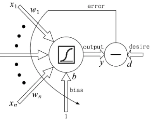
(2) Figure 1: Single neuron diagram. In the above equations w denotes the weight between two neurons. d is the desired response. x is the input. y denotes the neuron’s output. ¾ is the active function. ´ is a tunable learning rate. l denotes the number of layer, where 1 denotes the …rst hidden layer and L is the output layer. i or j denote the number of neuron in each layer. So, yjl is the output of the j 0 th neuron l is the weight between the j 0 th neuron in the l0 th layer and the in the l0 th hidden layer, wji i0 th neuron in the (l ¡ 1)0 th layer. blj is the j 0 th neuron’s bias. dlj is the desired response of the j 0 th neuron in the l0 th layer. ± lj is the j 0 th neuron’s delta value for weight correction. m0 is the number of neurons in input layer, ml¡ 1 is the number of neurons in the (l ¡ 1)0 th layer . All neurons use these equations to improve their weights. Each neuron use the outputs of all neurons in the next precedent layer as inputs. We will isolate each neuron with all its weights, inputs, desired response, and output. This allows us to implement the BP algorithm on distribute parallel machine. In the next section, we present the basic module for a single neuron. Then we show a data ‡ow [1] structure for multilayer networks constructed with such basic module.. 2. The basic module. Fig. 1 shows the diagram of a single neuron. The forward equation is: Ã N ! X t t t y =¾ wi xi + b. (6). i=0. where t denotes time and the active function is temporarily set to the bipolar sigmoid function ¾(u) = 1+e2¡ u ¡ 1. According to the delta learning rule [2][6], the error-correction function is de…ned by: ¢ wt = ´. 1 t (d ¡ y t )(1 ¡ (y t )2 )xt : 2. (7). And the weight is updated according to: wt+1 = wt + ¢ wt :. (8). Combining Eq. 6,7 and setting F be the updation function for this neuron, we obtain: (¢ wt ; y t ) = F(wt ; xt ; dt );. (9).

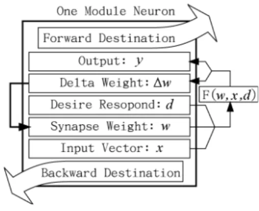
(3) Figure 2: One module neuron data structure where F uses w(weight), x(input), and d(desire response) as its inputs and ¢ wt and y t as it’s outputs. The data structure for this neuron is plotted in Fig. 2. This structure is well known among the engineering society.. 3. The modular design for multilayer networks. We can use this basic module to construct various kinds of neural networks, such as multilayer network [3], multilayer network with jump connection [3], recurrent network [8][9] and selforganized map [4]. In this section we show how to construct a multilayer network and recurrent network.. 3.1. Multilayer network. A multilayer network can be transformed into its modular form in O(n) time, where n is the number of total neurons. With a pointer supporting language, such as C [7], we can allocate a memory space for each neuron and maintain a pointer pointing to it. The algorithm is: algorithm Modular Transform for L=1 to number of layers for N=1 to the number of neurons in layer L Neu Ã allocate a memory space for each neuron. Store all data of this neuron(L; N) in Neu. Set Neu!forward destination point to neurons in next layer. Set Neu!backward destination to neurons in precedent layer. Look up table(N; L) Ã Neu’s location. end. end. end. Table 1: Modular Transform Algorithm. It is a little cost of memory doing this modular transform. Usually the BP algorithm is implemented using a matrix (or an array) to store weights, input vector and output vector. Each entry in the matrix corresponds to a neuron’s relative position in the network. Instead.

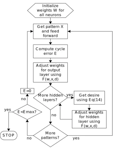
(4) of this matrix, we maintain a pointer for each neuron which contains the synapses to all linked neurons. The key part of the module is that the desired response for each neuron must be given in advance, not only for the neuron in the output layer. Therefore, the BP algorithm (equation 1 to 5) must be reformed in such a way that every hidden neuron can be treated like an independent neuron as long as we can calculate its desired response. For this response, observe the two equations; ±L j = ± lj. ¢ ¡ 1 L (dj ¡ yjL ) 1 ¡ (yjL )2 ; 2. (10). l+1 ´m X 1 ³ l+1 l 2 = 1 ¡ (yj ) ± il+1 wij : 2. (11). i=1. Equation 10 and 11 are the backward delta equation in the BP algorithm using the bipolar sigmoid function. Symbols are de…ned same as preceding section. Equation 10 is for the the neurons in the output layer and equation 11 is for hidden layer. Simplify these two equations, where we regard yjL and yjl as the same role, we obtain the desired response for each neuron in the hidden layer, ml+1. X. dlj = yjl +. l+1 ± il+1 wij :. (12). i=1. L = ´± L y L , the delta for the neuron i in the output layer is: According to ¢ wij i i. ±L i =. L ¢ wij. (13). ´yiL. Substitute equation 13 into 12 the desired response for the j 0 th hidden neuron is: ml+1. dlj = yjl +. l+1 X ¢ wij i=1. ´yil+1. l+1 wij ;. fl + 1 = 2::::Lg:. (14). With equation 14 we obtain all neurons’ desired responses no matter what layer it belonging to. Therefore each neuron can be treated separately. To our knowledge this equation has not been discussed before. In …gure 3, we illustrate a ‡ow chart of the modular design for the BP algorithm. The main di¤erence between the formal BP algorithm [2] is that we calculate each neuron’s desired response before adjust its weights. Figure 4 shows an example of a 1-3-2 modular design network. Similar to the multilayer feed forward network, a multilayer network can have jump connection (see …gure 5) from lower level to higher level. It’s forward and backward equations are similar to the BP equations 1 to 5. Its modular design is similar to that for the the multilayer feed forward network.. 3.2. Recurrent Network. A recurrent network [8][9] uses its outputs as its inputs. We show the modular design for training a recurrent network in Figure 6. The training procedure starts by feeding an input vector x into the modular network. The desired response is set to a target sequence. The output of the network is feedback to itself as the next input in each iteration. The procedure will be.

(5) Initialize w e ights W for all neurons G e t pattern X and feed forward. C o m p u te cycle error E A d just w e ights for output layer using F(w,x,d) E=0 M o re hidden layers?. no yes. STOP. E<Emax?. no. no. M o re patterns?. yes. G e t desire using Eq(14) A d just w e ights for hidden layer using F(w,x,d). yes. Figure 3: Modi…ed BP training ‡ow of modular design network.

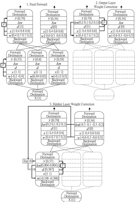
(6) Figure 4: Training procedure of modular design network. The values in step 1 are randomly generated. Succeeding steps change its values accroding to initial step..

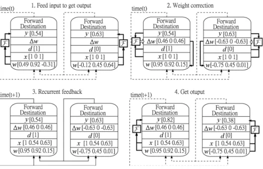
(7) Figure 5: An example of a multilayer network with jump connection. Figure 6: The training procedure of recurrent network using modular design. The values in step 1 are randomly generated. Succeeding steps change its values accroding to initial step..

(8) continued until the error reduced to a satis…able range. We treat recurrent network as a normal feed forward network, where we connect it’s output destination back to itself. The modular design is particularly useful for the data ‡ow machine. It is believed to achieve high degree of parallel computation. The main achievement is that we can decompose neural networks into small modules which enable us to feed each module into multi-speed processors that can conform the spirit of data ‡ow machine. The self-organization neural network can cope with the data ‡ow machine structure with less modi…cations and we omit its discussion.. References [1] Veen, Arthur H, (1986). Data‡ow Machine Architecture. ACM Computing Surveys, Vol. 18, No. 4, Dec., pp. 365-396 [2] D.E. Rumelhart, G.E. Hinton, and R.J. Williams (1968). Learning Representations by Backpropagation Errors. Nature(London), Vol. 323, pp. 533-536. [3] C.-Y. Liou. (2001). Lecture Notes on Neural Networks. National Taiwan University, 526 U1180. (http://red.csie.ntu.edu.tw//NN/index.html) [4] Kohonen, T. (1982). Self-organized Formation of Topologically Correct Feature Maps. Biological Cybernetics 43, pp. 59-59. [5] Volker Tresp, (2001). Committee Machines. Handbook for Neural Network Signal Processing, Yu Hen and Jenq-Neng (eds.), CRC Press. [6] McClelland, T. L., D. E. Rumelhart, and the PDP Research Group. (1986). Parallel Distributed Processing. Cambridge: The MIT Press. [7] Worthington, Steve (1988). C programming. Boston, MA : Boyd & Fraser Pub. Co. [8] Hop…eld, J. J. (1982). Neural Networks and Physical Systems with Emergent Collective Computational Abilities, Proc. Natl. Acad. Sci. 79: 2554-58. [9] Hop…eld, J. J. (1984). Neurons with Graded Response Have Collective Computational Properties Like Those of Two State Neurons. Proc Natl. Acad. Sci. 81: 3088-3092..

(9)