Robust digital design of continuous-time nonlinear control systems using adaptive prediction and random-local-optimal NARMAX model

Robust digital design of continuous-time nonlinear control systems using adaptive prediction and random-local-optimal NARMAX model

Zhi-Ren Tsai

Department of Computer Science & Information Engineering, Asia University, Taiwan Graduate Institute of Biostatistics, China Medical University, Taiwan

[email protected]

Abstract

In this paper the time-delay and uncertainty of continuous-time (CT) systems are considered, and it is suggested that input and output of a discrete- time (DT) Neural Plant Model (NPM) and recursive neural controller have scaling factors which limit the value zone of measured data from a system. Adapted scaling factors cause the tuned parameters to converge to obtain a robust control performance. However, the proposed Random-Local-Optimization (RLO) design for a model/controller uses off-line initialization to obtain a near global optimal model/controller. Other important issues are the considerations of cost, greater flexibility, and highly reliable digital products for these control problems. This issue of DT control design for CT plant is more difficult than that of CT control design for CT plant, because of the need to process the modeling error between the CT plant and DT model. The input-delay, uncertainty, and sampling distortion of a CT nonlinear power system need to be solved by developing a digital model-based controller. Here, this is called the DT tracking control design of CT systems (DT-CT).

Therefore, the DT structure of the adaptive controller for the CT nonlinear power system should be designed as a kind of feed-forward-Recursive-

Predictive controller (FRP). First, due to the problem of delays, a digital neural controller with feed-forward of the reference signal and a Nonlinear Auto- Regressive Moving Average eXogenous (NARMAX) neural model design is adopted to reduce this difficulty. The most important contribution is that the more reasonable and systematic two-stage control design, the CT nonlinear delayed system to be controlled is modeled using a NARMAX technique with the first-stage (off-line) method by the proposed global optimal network algorithm and second-stage (on-line) adaptive steps. Second, the dynamic response of the system is controlled by an adaptive NARMAX neural controller via a sensitivity function. A theorizing method is then proposed to replace the sensitivity calculation, which reduces the calculation of Jacobin matrices of the BP method. Finally, the feed-forward input of reference signals helps the digital neural controller to improve the control performance, and the technique works to control the CT systems precisely.

Keywords: Random-local-optimization algorithm, NARMAX model-based neural controller, DT-CT design

1. Introduction

During the past decade optimal control [1, 2] has attracted great attention from both the academic and industrial communities, and there have been many successful applications. Despite this success, it has become evident that many basic and important issues [3] remain to be further addressed. Of these, stability analysis and systematic designs are among the most important issues for optimal control systems [4] and robust control theories [1, 5-8], and there has been significant research on these issues (see [4, 9, 10]). In addition, a neural controller has been suggested as an alternative approach to conventional PID control techniques [11] for complex control systems [1].

Moreover, Neural-Network (NN) based modeling has become an active research field because of its unique merits in solving complex nonlinear system identification and control problems [10]. Neural networks (NNs) or NARMAX neural networks [12] are composed of simple elements operating in parallel, inspired by biological nervous systems. A neural network can be trained to represent a particular function by adjusting the weights between elements.

Due to discrete-time (DT) controllers being cheaper and more flexible than continuous-time (CT) controllers, the DT control problem for CT plant is worth studying. In modern control engineering, controllers are commonly implemented directly by the hardware or software of digital computers.

However, one important issue has to be faced; that is, the new design (DT-CT design) problem effects a new type of application, and an adaptive NN-model- based design method has not yet been developed to adjust the parameters of a discrete-time (DT) adaptive neural controller such that the original continuous-time (CT) system, with time delays and uncertainties, is uniformly ultimately bounded (UUB) stable.

The study of CT control of CT time-delay systems has received considerable attention in recent years since delay is a major cause of poor performance in many important engineering systems [13-15]. Hence, the future direction of CT time-delay control systems needs to involve the DT control problem. The amount of delay has different impacts on the various approaches [15-19]. As is known, the delay control problem is an important and complex factor in the stability performance of CT nonlinear systems. In general, a delay signal happens in a signal’s long-distance or heat translation.

Based on the timer of the micro-controller or Digital Signal Process (DSP) chip, the effect of delay in neural system identification can be approximated by many tape-delay terms. This reduces the difficulty of delay identification. The DT NARMAX model is general sufficient to approximate an unknown, nonlinear, dynamical and delayed CT system by selecting an appropriate sampling time.

DT control design for DT plant [20] and CT control design for CT plant are two kinds of well-known problems. [20] has inspired consideration of the more difficult problem of DT control design for CT plant, because of the need to process the modeling error between the CT plant and DT model, except for proposing the novel adaptive control law. The modeling and controlling performance can be guaranteed by the appropriate sampler and some theories. The modeling performance of plant is important for this research. The stability of results and the robust control design are related to this precise plant model. Hence, a two-stage training scheme is needed to guarantee a well- behaved model, referred to as a predictive controller. Based on this correct model, the control parameters can be updated by the BP method. That is one contribution of this paper. Another contribution is the proposal of a theorizing

Jacobin matrices of the BP method. That is why the adaptive prediction control method is used to improve the DT control performance of the proposed DT-CT design by tuning the parameters of the model and controller.

The feed-forward term in [20] is derived indirectly by assuming many constraints, and due to the over-fitting and local optimal problems of NN modeling, the method [20] is not suitable for on-line applications because of the need for a lengthy convergence time. Therefore, to satisfy the on-line working requirements for accurate modeling of the plant, the NARMAX plant and control models are trained by initially using off-line methods.

On the other hand, these neural techniques [21-23] have usually been demonstrated under nonlinear control due to their powerful nonlinear modeling capability [24] and adaptability. However, they must exhibit the optimal problem of falling into the local minimum easily by using the Back-Propagation (BP) or Levenberg-Marquardt BP algorithm (LMBP) [25] method. Hence, the RLO algorithm is proposed to improve this drawback. It not only guarantees the gradient decent method [26] against the local optimal solution, but also speeds up the convergence of the Particle Swarm Optimization (PSO) [31, 32].

Inspired by the DT neural controller of [20] only for a DT system, a digital neural control design for a CT system is proposed and an approximate inverse of the delayed plant dynamics is used to act as the NARMAX neural controller.

The adaptive controller and NARMAX models are easier to converge than [21- 23] by the proposed two-stage scheme. Moreover, the modeling error between the model and physical system is considered in the theorems by Lyapunov functions [27]. This paper concludes with a simulation example and experimental data to demonstrate these techniques.

2. System description

First, consider a general nonlinear system with delays; described as follows:

P: x(t )=f˙ _CT(x,u,t ,t−τ , Δ) and y(t )=g( x) , (1) where ^P shown in Fig. 1 is a controlled plant; the bounded uncertainties Δ(t) create the dynamic quality of the system parameters which refer to

electrical elements of the power system; the control input u(t) _; τ is the time delay; g(⋅) is the relational function of the state x(t ) and system

output y(t ) . Then, f_CT is discretized by setting the appropriate sampling

time or sampling period T_s (sec) of DTC-CTP design, and t=k⋅T_{s , where k}

is a positive integer, to the following DT nonlinear system f_{DT :} x((k+1)⋅T_s)=f_{D T}(x( k⋅T_s),u(k⋅T_s),T_s), y(k⋅T_s)=g ( x(k⋅T_s)) _or

x(k+1)=f_{D T}(x(k ),u(k),T_s), y(k )=g( x(k )) , (2)

where k indicates the signal sequence, the DT state vector is x(k⋅T_s) _{, and}

the DT control input is u(k⋅T_s) . The zero-order-hold control input u(t )=u (k⋅T_s)=u (k ) , where k is also the index of the discrete result u(k ) of

u(t ) referring to the NN model ^P (see Fig.1) of (1).

In this control structure in Fig. 1, the NN plant model is designed to approximate this nonlinear system Eq.(1). This NN plant model, or control model is built following the subsequent mathematical equations.

An NN plant model or control model with ^L layers each having N^l (

nonlinear system f^DT Eq.(2). Superscripts are used to distinguish between these layers. Specifically, the number of the layer is appended as a superscript to the name of the variable. Thus, the weight matrix for the l _{-th (} l=1,2,...,L ₎

layer is written as W^l and {W_P^l ,W_C^l }∈W^l . Moreover, it is assumed that v^r (

r=1^l,2^l,...,N^l ) is the net input and that all the transfer functions T^r(v_r) of units in the NN system are described by the following function:

T_r(v_r)=λ⋅

(

)

T_r(v_r)=v_r, for r=1^L,2^L,...,N^L _;

where ^q and λ are positive parameters associated with the sigmoid function. The transfer function vector of the l -th layer is defined as:

ψ^l(v_r)≡[T_r(v₁l),T_r(v₂l),...,T_r(v_Nl)]^T, l=1,2,...,L _,

where T^r(v_r) ( r=1^l,2^l,...,N^l ) is a transfer function of the ^r -th neuron. The

final outputs of the NN plant model ^P and control model C_F can then be inferred as follows: respectively:

^y(k )=ψ^L(W^Lψ^L−1(W^L−1ψ^L−2(...ψ²(W²ψ¹(W¹Z(T_s)))...)))

= ^P( y( k−1), y(k−2),..., y(k−n),u( k),u(k−1),...,u(k−p),W_P(k),T_s) _{, and} u_F=C_F(u(k−1),u(k−2),...,u(k−c_u),r( k),r(k−1),...,r( k−c_y),W_C(k ),T_s) _,

where r(k ) is a reference input,

Z^T(T_s)=[g(x((k−1)⋅T_s)),g( x((k−2)⋅T_s)),...,u(k⋅T_s),u((k−1)⋅T_s),...,1] _,

the adaptive parameter W^P(k)=[ W¹_P,W²_P,...] or W_C(k )=[W_C¹,W_C²,...] of neural

weights’ and biases’ refers to the iteration k and the proposed adaptive laws for the controller and plant models are as follows:

W_C(k+1)=W_C(k )+ΔW_C(k) _{, and} W_P(k+1)=W_P(k)+ΔW_P(k) _.

Although ΔW^P(k ) and ΔW_C(k) are the proposed adaptive laws of plant model and control model, respectively, where:

ΔW_P(k )=−η_P⋅( ^y(k )− y(k )) d ^y(k )

dW_P(k ) _, ΔW_C(k)^T=−η_C⋅( ^y(k)−r(k )) d ^y( k) dW_C(k) _,

but implementing

d ^y(k)

dW_C(k ) needs too many Jacobin matrices’ calculations, so

the following adaptive prediction control law is used

ΔW_C(k)^T=η_Xu_X du (k ) dW_C(k ) _to replace the above adaptive laws to reduce computing time,

where η_P, η_C, η_{X are learning rates;}

u_X=C_X(e( k))=[ K₁(e₁(k)), K₂(e₂(k )),K₃(e₃(k)),...]^T

is the predictor output, where the tracking error is e(k)=r(k )− y(k ) _{, and} e(k)=[ e₁(k ),e₂(k),e₃(k ),...]^T _, K₁(⋅), K₂(⋅),K₃(⋅),... are defined by the user.

A composite controller, u(k )=u_F+s⋅u_{X , where} s={0,1} is proposed in the next section.

3. Control architecture, neural-model-based controller design and control scheme

3.1 Adaptive digital neural controller design through neural plant model

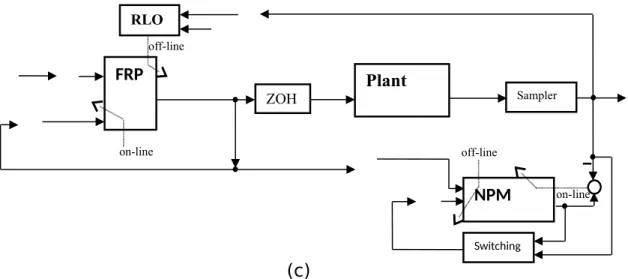
In this paper an adaptive prediction control structure is proposed, as shown in Fig. 1, where the FRP controller ^CF is designed as follows:

u(k )=u( z(k ))=C_F(z(k ),W_C(k ),T_s)+s⋅C_X(e(k ))=u_F+s⋅u_X , (3)

where e(k)=r(k )− y(k ) , the switch index

0 , {~e 1 , { ~¿ e

¿

¿

s =¿{(k +1 )≥0,¿ ¿ ¿

¿ And,

u( ^z(k ))=C_F( ^z( k),W_C(k),T_s), (4)

where u_P=u_F+u_{X ,} ^y₁(k+1)= ^P(u_P(k+1)) _, ^y₂(k+1)= ^P(u_F(k+1)) _, e^₁(k+1 )=r( k+1)− ^y₁(k +1 ) _, e^₂(k +1 )=r( k +1)− ^y₂(k +1 ) _,

|^e₁(k+1)|−|^e₂(k+1)|=~e(k+1) , as shown in Fig. 1. The feed-forward terms are

reference signals [r( k),r(k−1),...,r( k− p)] , and recursive terms are control

signals [u( k−1 ),u(k−2),...,u (k−q )] . The off-line training input of controller is:

^z(k)=[ y(k ), y(k−1),..., y( k− p),u(k−1),u(k−2),...,u( k−q)] _, The on-line recursive input of controller is:

z(k)=[ r(k ),r( k−1),. ..,r(k−p),u(k−1),u(k−2),...,u(k−q)] . The controller has two

working phases: z(k) is the data vector of the testing phase, and ^z(k) is the data vector of the training phase. The tuned parameter vector of the controller

is: W_C(k ) _{of (3).}

The proposed on-line digital neural controller u(k ) has feed-forward terms [r( k),r(k−1),...,r( k− p)] and recursive structure [u( k−1),u(k−2),...,u(k−q)] _. Hence, it uses a NARMAX neural model or inverse of the plant dynamics to aid control precision in the face of a delayed plant with uncertainties. Adapting the

neural controller can suppress the uncertainty of the plant P shown in Fig. 1.

Although the structure of the neural controller is chosen as (3), the neural

controller has not been designed because the parameter vector W_C(k ) _{is not} specified. ^γ⋅Ts is the chosen tape-delay time, γ is a positive integer. The idea of the inverse-model-based neural controller is proposed by the following simplified relation:

If y(k )= ^P(u(k )) _, ^{u(k )= ^P−1(r(k ))=C}_F^{(r(k ))} _{, then} y(k )=r(k ) , (5) where ^P(⋅) is the adaptive NARMAX neural model of plant; C^F(⋅) is the

adaptive NARMAX neural controller; r(k ) is the desired output. According to

the idea of Eq.(5), the recursive structure ^P(⋅) can be designed with tape delays as follows:

y(k )≈^y(k )= ^P( ^y( k−1), ^y(k−2),..., ^y( k−n),u(k),u(k−1),...,u( k−p),W_P(k ),T_s) _{, (6)}

where n, p+1 are the amount of tape delays of ^y ,u , respectively.

But, due to the parameters of the recursive structure are converged much

harder, the weights and biases W_P(k) of this model are trained by the feed- forward structure as follows:

^y(k )= ^P( y(k−1), y(k−2),..., y(k−n),u(k ),u(k−1),...,u(k−p),W_P(k),T_s) . (7) The plant output is compared with the desired output to create a tracking error

signal e(k)=r(k )− y(k ) . The system errors e(k)=r(k )− ^y(k )^ _and e(k) _{are used}

by the adaptation algorithm to update the parameters of ^P and C_{F . Next,} the performance index for minimizing the tracking error is designed, as follows:

J (k )=1

2e(k )^Te(k )=1

2(r (k)− y(k ))^T(r(k )− y( k))=1

2(y(k )−r( k))^T(y(k)−r(k ))

, (8) is a simple cost function to be minimized by the proposed algorithm. Then, the

on-line BP algorithm adapts the control parameter matrix W_C(k ) . That is, the

change in control parameters ΔW_C(k) is calculated as ΔW_C(k)^T=−η_C(k ) dJ (k )

dW_C(k)=−η_C(k )d( y(k )−r (k))^T(y(k )−r(k )) 2⋅dW_C(k)

=−η_C(k )( y (k )−r (k )) dy (k )

dW_C(k )=−η_C(k )( y (k )−r(k ))dy (k ) du(k )

du( k )

dW_C(k ) , (9)

where the small positive η_C(k ) can be selected as a stable learning rate via the following theorems.

Theorem 1: If the number of neurons and tape-delay terms of the neural

model is sufficient, and the appropriate sampling time T_s is selected to let

‖¯y(k )−y(k)‖≤¯ε and the following condition

0<η_P(k )< 2

‖ d ^y(k ) dW_P(k)‖

2≤¯η_P

, (10) is satisfied, where

d ^y ( k)

dW_P(k)= ∂ ^y(k )

∂W_P(k )+∑

i=0 p_u

∂ ^y (k )

∂u (k−i )

du(k −i) dW_P(k )+∑

i=1 p_y

∂ ^y (k )

∂ ^y (k−i )

d ^y(k −i) dW_P(k ) ;

¯y(k ) is the output of the optimal model, then the trajectories ^y(k )

converging to plant output y(k ) is a uniformly ultimately bounded (UUB)

approximation on the bounded error ^y(k )− y(k ) _.

3.2 Proof of Theorem 1

First, consider the following ideal Lyapunov candidate [27] for the model part,

V₁(k )=1

2( ^y(k)− y(k ))^T( ^y(k )− y(k ))=1

2‖^y(k )−¯y(k )+¯y(k )−y(k )‖²

=1

2‖ ^y(k )−¯y(k )‖²+ε(k )=V₂(k)+ε(k )

, (11)

where V₂(k)=1

2‖ ^y(k )−¯y(k )‖²

is an actual Lyapunov candidate of reachable and

assumptive trajectory ¯y(k ) , the bounded approximation error ε( k)=1

2‖¯y(k )− y(k )‖²+( ^y(k )−¯y(k ))^T( ¯y( k)− y(k)) ,

and the number of neurons of the neural model is sufficient and the

appropriate sampling time T_s is selected to let ¯y (k )≈ y (k ) . The next task is

to train this neural model such that V₂(k) is minimized, ΔW_P(k )

η_P(k ) =−( ^y(k )− y(k )) d ^y( k) dW_P(k)

¿− dV₂(k )

dW_P(k )=−( ^y ( k )−¯y(k))d ( ^y (k )−¯y (k ))

dW_P(k ) =−( ^y (k )−¯y(k )) d ^y (k )

dW_P(k ) . (12) Then, the following Lyapunov candidate for the controller is designed:

V₃(k)=1

2( ^y(k )−r(k ))^T( ^y( k)−r(k ))=1

2‖ ^y(k)−r(k )‖²

, (13) thus the change in the Lyapunov function is obtained by:

V₃(k+1)−V₃(k )=1

2(‖^y(k+1)−r(k+1)‖²−‖ ^y(k)−r(k )‖²)

. (14) Finally, the update law of the control parameters of the controller is obtained as follows:

ΔW_C(k )^T

η_C(k ) ≈− dV₃(k )

dW_C(k )=−( ^y( k)−r(k )) d ^y(k )

dW_C(k) . (15) This study develops some convergence theorems to select appropriate stable

learning rates. First, the difference of modeling error e_P(k )= ^y( k)−¯y( k) _{can be} represented by

e_P(k +1 )=e_P(k )−

[

]

[

]

(

[

]

)

=e_P(k )

(

[

]

)

thus the change in the Lyapunov function is obtained by:

V₂(k+1)−V₂(k )=1

2(‖e_P(k+1)‖²−‖e_P(k)‖²)=1

2

(

⁽

^[

^]

⁾

)

=1

2‖e_P(k )‖²

[ ⁽

^[

^]

⁾

]

Hence, if

−1<

(

[

]

)

V₂(k+1)<V₂(k) , that is V₂(k )→0 _or ^y(k )→¯y( k) , makes the UUB

approximation of this model on the bounded ^y(k )−y(k ) . The proof is thereby completed.

Furthermore, the following theorem for the convergence of the controller is obtained by the same procedure as the above proof.

Theorem 2: If Theorem 1 in Eq.(10) is satisfied, the function

d ^y(k)

dW_C(k ) in Eq.

(15) is computed to let the following condition,

0<η_C(k)< 2

‖ d ^y(k ) dW_C(k )‖

2≤¯η_C

, (17) be satisfied.

Where

d ^y (k ) dW_C(k )=∑

i =0 p_u

∂ ^y (k )

∂u(k −i)

du(k −i) dW_C(k )+∑

i=1 p_y

∂ ^y(k )

∂ ^y (k −i)

d ^y( k−i) dW_C(k ) ,

with

du( k )

dW_C(k )= ∂u(k )

∂W_C(k )+∑

i=1 c_u

∂u( k )

∂u( k−i)

du (k−i) dW_C(k ) ,

then the nonlinear systems (1) in Fig. 1c are UUB stable, and the tracking errors e(k)=r(k )− y(k ) are bounded via the controller.

Hence, the dynamic response of the system P can be controlled using C_F , as shown in Fig. 1. This C_F needs the plant model ^P to adjust control

parameters via sensitivity function

∂ ^y(k )

∂u(k−i) _.

The digital feedback controller includes a delay block D, as shown in Fig. 1.

Here, the error ~e(k+1) is used to estimate u_X , and the proposed predictor of the delayed system can let us cancel some complex computations, such as

∂ ^y(k+1 )

∂u(k+1 )≈y( k+1)− ^y(k)^

Δu(k+1) =Δ ^y(k+1)

Δu( k+1)=Δ ^y(k+1) u_{X ,}

of sensitivity function

∂ ^y(k )

∂u(k−i) in the BP algorithm. Hence, the following theorem is proposed to update the control parameters of FRP under the assumption of providing a model which applies a lower prediction error, and a

more correct u_X . The prediction error e(k+1)=r(k+1)− ^y(k+1)^ is bounded,

due to the previous e(k)=r(k )− ^y(k )^ being bounded at any time. Hence, the

prediction error e(k+1)^ will be bounded by using Theorem 1-2. Furthermore, the following theorem is obtained for the convergence of the adaptive prediction controller by the same procedure as Theorem 1.

Theorem 3: If Theorem 1 in Eq.(10) is satisfied, the predictive function

du( k+1)

dW_C(k+1) is computed to let the following condition,

0<η_X(k+1 )< 2

‖ du(k +1 ) dW_C(k+1)‖

2≤¯η_X

, (18) be satisfied, then the nonlinear systems (1) in Fig. 1a-1b are UUB stable, and

the tracking errors e(k)=r(k )− y(k ) are bounded via the predictive controller

u(k+1)=u_F(k+1)+s⋅u_{X .}

The tracking error is e(k)=r(k )− y(k ) _{, and} ^{e(k)=[ e}1(k ),e₂(k),e₃(k ),...]^T _{, but the}

parameters of adaptive control C_F are updated by using the predictive offset

Δu(k+1)=u_p−u( k)=u_X=C_X(e(k ))=[ K₁(e₁(k )), K₂(e₂(k)), K₃(e₃(k )),...]^T _,

of the prediction control input u_p=u( k+1) _{, where}

∂ ^y(k+1 )

∂u(k+1)≈y( k+1)− ^y(k)^

u_p−u(k ) =Δ ^y(k+1)

u_X replaces

d ^y(k )

du(k ) in the following recursive equation:

d ^y (k )

dW_C(k )=d ^y (k ) du (k )

du( k ) dW_C(k )=∑

i=0 p_u

∂ ^y (k )

∂u(k −i)

du(k −i) dW_C(k )+∑

i=1 p_y

∂ ^y (k )

∂ ^y (k−i )

d ^y (k −i)

dW_C(k ) , therefore, only

du( k)

dW_C(k ) or

du( k+1)

dW_C(k+1) need to be calculated to update W_C(k ) _or W_C(k+1) _, respectively, and K₁(⋅), K₂(⋅),K₃(⋅),... are defined by the user.

3.3. Two-stage scheme

Fig. 1 shows a block-diagram of an adaptive recursive control system. The system to be controlled is labeled as the plant P , which is subject to uncertainties and delays. Due to gradient-descent based training algorithms, let the model/controller converge to a local minimum in the solution space.

Hence, the two-stage training algorithm is proposed, as follows.

In the first stage, the measured data is used to train the global optimal NARMAX plant and neural controller by the training-data-shuffle method. This method shuffles the training data to avoid most of the local optimal solutions obtained by the off-line training procedure in next section. The measured data

used for training the NN. However, the final performance of the NN is decided by the testing data and the training data.

In the second stage, the global optimal NARMAX plant model and neural controller is adapted. The two stages are divided into the following five steps:

Step 1: First, the reference signal, r(k ) , is designed. By the white noise of

input u(k ) for plant, output data y(k ) is collected and a training-data- shuffle method is used to shuffle the input/output pairs’ data. These shuffled data are ready to train the NARMAX model/controller. Here, the following reasonable conditions need to be taken into account:

max

k (r (k))≈max

k (y(k ))

, min

k (r(k ))≈min

k (y( k))

, max

k (u (k))≤u_U

, and min

k (u(k ))≥u_L

,(19) need be satisfied, where u_U is the upper bound of u(k ) _{, and} ^uL is the

lower bound of u(k ) . According to Eq.(19), much of the excessive

control effort u(k ) can be avoided. If Eq.(19) is satisfied, then go to Step 2.

Step 2: The feed-forward structure model ^P is trained/tested off line

^y(k )= ^P( S_uu( k),S_uu(k−1),...,S_uu(k−p_u), S_yy(k−1), S_yy(k−2),...,S_yy( k−p_y),W_P(k),T_s)(1/S_y),

(20) via the shuffled input/output pairs’ data. After system identification ^P

is performed, and the digital neural controller C_F for the CT system can be built by using this inverse NARMAX plant model ^{^P−1} in the next step.

Step 3: In practice, according to the exchanged output/input pairs’ data from Step 2, the off-line stage to train/test the neural controller can be passed through

u(k )=C_F(S_uu(k−1),S_uu(k−2),...,S_uu(k−c_u),S_yy( k),S_yy(k−1),...,S_yy(k−c_y),W_C(k),T_s)(1/ S_u)

. (21) If Eq.(20) and Eq.(21) work, go to Step 4.

Step 4: Update the on-line weights and biases W_P

of the recursive structure model ^P :

^y(k )= ^P( S_uu( k),S_uu(k−1),...,S_uu(k−p_u), S_y^y(k−1), S_y^y(k−2),...,S_yy( k−p^ _y),W_P(k),T_s)(1/S_y),

(22) to approximate the CT nonlinear system by using Remark 1 and Theorem 1. Due to the adaption laws for Eq.(20) and Eq.(22), an exchange for both of them can be designed to switch into the system, as a switching in Fig.

1, when Eq.(22)’s absolute approximation error is too big. If Eq.(20) and Eq.(22) work, then go to Step 5.

Step 5: Adapt the digital neural controller for the modeling error and tracking error by using Remark 1 and Theorem 1-2. Finally, update the on-line

parameters of the neural controller C_F

u(k )=C_F(S_uu(k−1),S_uu(k−2),...,S_uu(k−c_u),S_yr (k),S_yr (k−1),...,S_yr( k−c_y),W_C(k ),T_s)(1/S_u) _,

(23) to minimize the tracking error, and finish the above two stages: the off- line stage and on-line stage.

To make sure of the robustness of the control system, the convergence to the global optimal solution of parameters of the model/controller has to be

guaranteed. Hence, some random initial weights and biases of the model are designed by Particle Swarm Optimization (PSO) [31, 32] with the parameters of the controller first. The PSO algorithm consists of the velocity

v_i(j+1)=v_i(j)+γ_1i⋅(p_i−¯x_i(j))+γ_2i⋅(G−¯x_i(j )) _,

and position

¯x_i(j+1)=¯x_i(j)+v_i(j+1) _,

where i=1,2,...,H is the particle index; j=1,2,..., N is the iteration index; v_{i is}

the velocity of i th particle; ¯x_i is the position of i th particle; p_i is the best position found by i th particle (personal best); G is the best position found

by the swarm (global best, best of personal best); γ_1i,γ_2i are the random numbers on the interval [0,1] applied to the i th particle.

The PSO supplies random initial parameters, hence, it is an initial parameters’ conductor. These initial parameters are then converged locally by the LMBP method and the best solution for the initial model/controller is chosen. Finally, the global optimal solution of parameters can be found every time. Hence, this idea has been named the Random-Local-Optimization (RLO) algorithm. The RLO algorithm is a composite of the LMBP algorithm and a random initialization procedure of evaluating fitness value 1/( Ξ+0.01) , where Ξ=ρ⋅Ξ₁+(1− ρ)⋅Ξ_{2 ,} ρ∈[ 0,1] . The total of absolute training error Ξ_{1 is}

obtained by LMBP via the training data, and Ξ₂ is the total of absolute testing error of the model/controller output via the testing data input. In this paper, off- line RLO is used as a learning algorithm for the feed-forward structure model

plant model being not converged. After the off-line training stage, in order to

tune on-line the parameters of the plant model Eq.(22) recursively,

d ^y( k) dW_P(k) _of Eq.(10) needs to be calculated as follows:

d ^y ( k )

dW_P(k )= ∂ ^y(k)

∂W_P(k )+∑

i=0 p_u

∂ ^y(k )

∂u (k−i )

du(k −i) dW_P(k )+∑

i=1 p_y

∂ ^y (k )

∂ ^y (k−i )

d ^y(k −i)

dW_P(k ) . (24) Similarly, in order to tune the on-line parameters of the controller Eq.(23)

recursively, and

d ^y(k)

dW_C(k ) of Eq.(18) needs to be calculated as follows:

d ^y (k ) dW_C(k )=∑

i =0 p_u

∂ ^y (k )

∂u(k −i)

du(k −i) dW_C(k )+∑

i=1 p_y

∂ ^y (k )

∂ ^y (k −i)

d ^y ( k−i)

dW_C(k) , (25)

where

du( k )

dW_C(k )= ∂u(k )

∂W_C(k )+∑

i=1 c_u

∂u( k )

∂u( k−i)

du (k−i)

dW_C(k ) . (26) Hence, the following algorithm adapts a NARMAX neural controller for a NARMAX neural model of plant.

Step 1: Back propagate through C_F to form

∂u(k )

∂u(k−i) _and

∂u(k)

∂W_C(k ) _{in Eq.}

(26). If update

du( k)

dW_C(k ) of Eq.(26), and shift

du(k−i)

dW_C(k) down in Eq.(25), then go to Step 2.

Step 2: Back propagate through ^P _{to form}

∂ ^y(k )

∂u(k−i) _and

∂ ^y(k )

∂ ^y(k−i) _{in Eq.}